Analysis of the Impact for Mixed Traffic Flow Based on the Time-Varying Model Predictive Control

Abstract

The connected and automated vehicles (CAV) smoothing mixed traffic flow has gained attention, and a thorough assessment of these control algorithms is necessary. Our previous research proposed the time-varying model predictive control (TV-MPC) strategy, which considers the time-varying driving style of human driven vehicles (HDV), performing better than current baseline models. Due TV-MPC can be applied to any traffic congestion scenario and the dynamic modeling that considers driving style, can be easily transferred to other control algorithms. Thus, TV-MPC enable to represent typical control algorithms in mixed traffic flow. This study investigates the performance of TV-MPC under diverse disturbance characteristics and mixed platoons. Firstly, quantifying mixed traffic flow with different CAV penetration rates and platooning intensities by a Markov chain model. Secondly, by constructing evaluation indicators for micro-level operation of mixed traffic flow, this paper analyzed the impact of TV-MPC on the operation of mixed traffic flow through simulation. The results demonstrate that (1) CAV achieve optimal control at specific positions within mixed traffic flow; (2) higher CAV penetration enhances TV-MPC performance; (3) dispersed CAV distributions improve control effectiveness; and (4) TV-MPC excels in scenarios with significant disturbances.

1. Introduction

High traffic demand scenarios frequently experience unexpected interruptions. When passing through congested sections, vehicles often undergo forced deceleration and acceleration. This stop-and-go phenomenon can severely impact traffic operations. Moreover, extensive research has demonstrated that speed oscillations in traffic flow can increase travel time, elevate collision risks, escalate fuel consumption and emissions, as well as reduce driving comfort [1,2,3]. However, the development of Connected and Autonomous Vehicles (CAV) and intelligent transportation systems presents possibilities for solving these issues [4,5,6].

Therefore, numerous researchers, based on in-depth theoretical studies and empirical analyses, have proposed a series of innovative strategies to control CAV, aiming to utilize CAV to prevent the propagation of traffic disturbances and guide following vehicles within a fleet. Among the control strategies for CAV, the research on Jam-Absorption Dynamics (JAD) [7,8] and Leading Cruise Control (LCC) [9] has been the most representative in recent years. In practice, the decisions of CAV impact the subsequent driving behavior of human driven vehicles (HDV). Under the JAD strategy, CAV mainly act as followers, overlooking their potential role as leaders. While the LCC method has effectively addressed this issue. The early LCC faced limitations due to fixed parametric models, primarily based on traditional car-following models (such as the IDM model) that assume traffic flow behavior follows fixed rules [10,11]. However, the randomness of human driving behavior (such as aggressive lane changes and irrational deceleration) leads to model prediction failures. Many recent studies focus on developing learning-based models to more accurately capture and predict the behavior of HDV, thereby designing platoon controllers [12,13,14]. Our previous time-varying model predictive control (TV-MPC) strategy achieved a more accurate modeling of HDV by considering its time-varying driving styles [15]. This cause to address the issue of low accuracy in predicting HDV driving behavior.

However, this type of research focuses on proposing new methods, with the experiments conducted more aimed at demonstrating the advantages of the proposed methods. There is a lack of comprehensive evaluation regarding the impact of different traffic compositions and penetration rates on aspects such as environmental protection, comfort, safety, and efficiency, in order to clarify the effects of this algorithm on traffic and the benefits under different scenarios. Therefore, this paper will conduct a comprehensive analysis of the impact of the TV-MPC strategy on the microscopic operational states of mixed traffic flow. Considering the research topic of this paper, the focus is mainly on two key points: quantitative characterization of mixed traffic flow and exploring the applicable scenarios of control strategies.

Ensuring the characterization of mixed traffic flow with different CAV penetration rates and platooning intensities is essential. Furthermore, how to conduct reasonable experiments and select appropriate evaluation indicators to conduct in-depth research on the applicable scenarios of control strategies is crucial. The main contributions of this paper are reflected in the following two aspects:

1. Based on the TV-MPC longitudinal control strategy, different scenarios are designed to explore the impact of various characteristics of disturbances and platoons on traffic efficiency, traffic oscillations, fuel consumption, and pollutant emissions in mixed flow.

2. The results reveal the nonlinear relationship between the optimal positioning mechanism, penetration rate, and effectiveness of CAV in mixed traffic flow, as well as the favorable performance of CAV’s dispersed distribution.

The remainder of this paper is organized as follows: Section 2 reviews related studies. Section 3 discusses and validates the description of mixed traffic flow with different CAV penetration rates and platooning intensities based on the Markov chain model. An evaluation index system has been established in Section 4. Section 5 explores the impact of CAV positioning, platooning intensity, CAV penetration rate, and various degrees of disturbances on mixed traffic flow based on the TV-MPC longitudinal control strategy. Section 6 proposes recommendations and applications for the TV-MPC strategy. The Section 7 is the conclusion of this paper.

2. Literature Review

2.1. Research on Leading Cruise Control

In practice, the decisions of CAV impact the subsequent driving behavior of HDV. Under the JAD strategy, CAV mainly act as followers, overlooking their potential role as leaders [16,17]. Therefore, Wang et al. proposed a LCC control framework that not only takes into account the trajectory information of leading vehicles but also explicitly considers the influence of CAV’ own behavior on upstream traffic, namely the following vehicles behind the CAV, thereby addressing this research gap effectively [18]. Consequently, CAV equipped with LCC can guide the driving of following vehicles, facilitating a smoother mixed traffic flow. Building on this, a recent approach combining Data-Enabled Predictive Control (DeePC) [19] with the LCC framework integrates constraints based on speed error and distance error to enhance traffic performance [20]. This method is based on behavioral system theory [21] and Willem’s fundamental lemma [22] to bypass the explicit model description of HDV, instead relying on an implicit description of system trajectories. Extensive simulations have demonstrated the potential of Data-enabled predictive leading cruise control (DeeP-LCC) in mitigating traffic fluctuations, reducing fuel consumption and ensuring safety. Besides a rigorous controllability and observability analysis of DeeP-LCC has been conducted in [23].

To address the unknown disturbances from the head vehicle, Stefan et al. performed a min-max robust optimization on Deep-LCC, which improved the control effects, yet the overall noise problem in traffic has not been adequately resolved [24]. Accessibility analysis can withstand all possible noise and disturbances. Building on the study by [23], Shang et al. proposed a robust data-supported predictive method for advanced cruise control based on accessibility analysis, effectively reducing traffic flow oscillations by addressing noise and disturbances [25]. However, existing research predominantly relies on simulation for validation [26,27]. The research conducted real-world experiments based on a micro-traffic platform, considering the penetration rate and spatial positioning of CAV, demonstrating the applicability and advantages of DeeP-LCC [28].

2.2. Quantitative Description and Impact Analysis of Mixed Traffic Flow

In terms of describing mixed traffic flow, theoretical modeling has become the preferred method for most scholars studying the capacity of mixed traffic flow. Chen et al. [29] mainly considered the impact of CAV penetration rate and queue size on road capacity. The research results indicated that the road capacity of mixed traffic flow increases with the rise in CAV queue size; however, this queue size should not exceed 10. Based on this, Zhu et al. conducted an in-depth study on how CAV penetration rate and queue size affect road capacity and traffic congestion levels, revealing that optimal CAV penetration rate and queue size can maximize road capacity [30]. Sharma and other scholars shifted their research focus to the impact of human drivers’ self-awareness on mixed traffic flow. Three evaluation indicators were used when assessing the effects of mixed traffic flow: the level of traffic flow interference, efficiency, and safety [31].

Besides, substantial literature has examined the impact of various factors on traffic flow. Studies have indicated that an increase in the penetration rate of CAV can further enhance the stability and disturbance rejection capabilities of mixed traffic [32,33,34,35]. Zong et al. demonstrated through numerous numerical simulations that the position of CAV within a platoon and different disturbance characteristics can affect the carbon emissions of subsequent vehicles in mixed traffic [36]. In fact, each vehicle in a platoon contributes differently to energy savings, and CAV do not necessarily have to travel continuously; they can be distributed at any position within mixed traffic. Therefore, the spatial distribution of CAV affects mixed traffic flow. In recent years, scholars have explored the impact of CAV spatial distribution using theoretical analysis and traffic simulation. For example, Li et al. used a set function optimization method to study the optimal platooning of multiple autonomous vehicles and found that both uniform distribution and queue formation are two optimal formations. Another factor that may significantly affect mixed traffic flow is platoon intensity. Platoon intensity reflects the degree to which vehicles in a platoon travel on the road. The magnitude of platoon intensity is related to the communication and control capabilities of autonomous vehicles. Even at the same CAV penetration rate, different spatial arrangements of CAV can lead to different platoon intensities, thereby affecting the operational status of mixed traffic flow [37,38]. Ghiasi et al. were the first to apply Markov chains to characterize the heterogeneity of mixed flows and the spatial distribution of random headway times, theoretically proving that this method can quantify mixed traffic flows with varying CAV lane intensities and penetration rates [39]. Subsequently an analytical framework between capacity, CAV penetration rate, and platoon intensity was constructed based on this foundation [40]. Yao et al. utilized Markov chains to describe mixed traffic flow involving HDVs, CAV and AVs. The proposed model can calculate the probability of CAV for any fleet size within the mixed traffic flow [41].

In summary, existing research lack a comprehensive characterization analysis of mixed traffic flow based on LCC technology. While our previous research proposed the TV-MPC strategy, which considers the time-varying driving style of HDV based on LCC, performing better than current baseline models. Therefore, this paper will conduct a comprehensive impact assessment of mixed traffic flow operations based on TV-MPC. Considering the research topic of this paper, the focus is mainly on two key points: quantitative description of mixed traffic and exploring the applicable scenarios of control strategies.

3. Quantitative Description of Mixed Traffic Flow

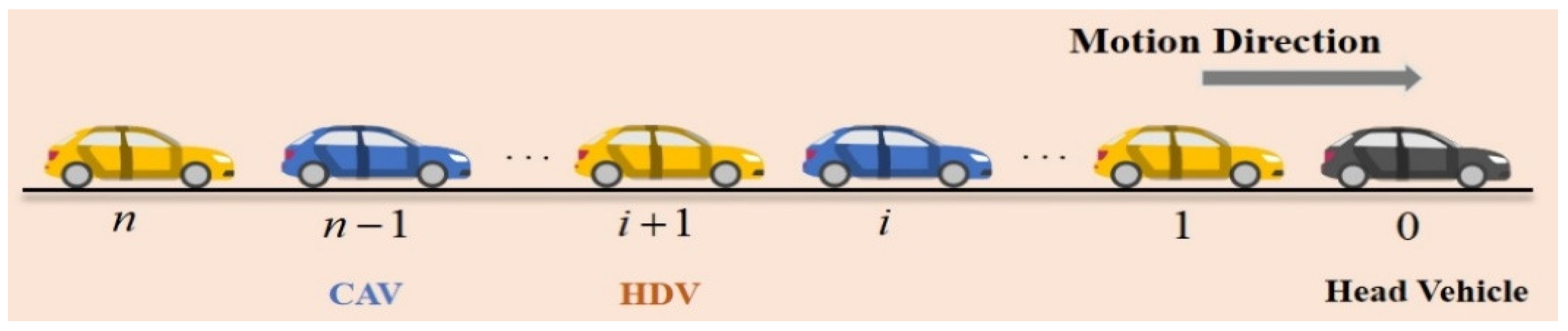
3.1. Problem Statement

In order to conduct a comprehensive analysis of the operational state of mixed traffic flow influenced by LCC technology, this study takes into account the long-term coexistence of HDVs and CAV within the traffic system. Thus, the research focuses on mixed traffic flow, employing a Markov chain model to quantitatively describe mixed traffic under varying CAV penetration rates and vehicle queue intensities. Based on this, the study examines the impacts of different fleet characteristics and the degree of headway disturbance on the capacity, stability, traffic safety, and environmental protection of mixed traffic flow within the TV-MPC (Traffic Vehicle Model Predictive Control) framework. Figure 1 provides a specific description of the research subject addressed in this paper.

As show in Figure 1, the general mixed traffic flow consists of $n+1$ vehicles, where exists one CAV, $n-1$ HDVs and one head vehicle. Then the head vehicle is defined as the index of 0, and the indices of the following vehicles are sequentially defined as 1 through $n$. Define sets $H$ and $C$ as type-HDVs and type-CAV respectively. $x_i\left(t\right)$, $v_i\left(t\right)$, $a_i\left(t\right)$ and $s_i\left(t\right)$ denote the position, velocity, acceleration and intervehicle spacing of vehicle $i$ at time $t$.

3.2. Markov Chain Model

Considering a mixed platoon Consider a mixed platoon of N following vehicles moving in a straight line along a highway, where the index 0 represents the leading vehicle, and the indices of the remaining following vehicles are $N=1,2,\dots ,n$. For convenience, we introduce the notation $A_i\in \left\{0,1\right\}$ to represent the type of vehicle in the platoon; if the i-th vehicle is a CAV, then $A_i=1$, and $A_i=0$ indicates that the i-th vehicle is an HDV The penetration rate $P_1$ is defined as the expected percentage of cars among all vehicles, that is,

$$P_1={\rm E}\left({\displaystyle \sum _{i\in \mathbb{N}}{A}_i/N}\right)$$

(1)

Therefore, the corresponding percentage of HDVs among all vehicles can be defined as:

$$P_0={\rm E}\left({\displaystyle \sum _{i\in \mathbb{N}}\left(1-A_i\right)/N}\right)=1-P_1$$

(2)

It is important to note that even with the same number of vehicles in a mixed platoon, the arrangement of vehicles is not unique under the same CAV penetration rate. The same value of $P_1$ may correspond to different distributions of vehicle types or the platoon intensity of CAV. For example, when the penetration rate of CAV is 50%, i.e., $P_1=0.5$, one extreme scenario is that the platoon forms a segregated pattern of CAV and HDVs, where each CAV is exactly separated by an HDV (as shown in Figure 2a), which represents the weakest clustering intensity. Another extreme scenario is that CAV and HDVs are completely separated, with the first half of the platoon consisting entirely of CAV and the remaining vehicles being HDVs (as shown in Figure 2b). This scenario represents the maximum platoon intensity. In contrast, as depicted in Figure 2c, the arrangement of CAV and HDVs is random, with the clustering of CAV occasionally interrupted by HDVs.

In summary, under the same CAV penetration rate, there are many corresponding situations with different queuing intensities. In each case, the control output of CAV will vary due to the different positions of CAV in the queue, which may affect the ability of CAV to dampen smooth traffic oscillations. To succinctly simulate the general CAV platoon intensity in random mixed traffic, a discrete Markov chain model is used to sequentially designate the types of $n$ vehicles from downstream to upstream as follows. In this Markov chain, $A_i$ can be interpreted as the state variable at the i-th step, with the state space being:

$$S=\left\{1,0\right\}$$

(3)

where 1 and 0 denote the CAV and HDV type respectively. If the ahead vehicle is HDV type, the state space will be $\left[\begin{array}{cc}0& 1\end{array}\right]$ when the ego vehicle is CAV.

Due to the type of the first vehicle is unsure, we definite initial state (the first vehicle type) is:

$$\omega =\left[P_1,P_0\right]$$

(4)

Then the following transition matrix can be described by (5).

$$T=\left[\begin{array}{cc}{t}_{cc}& t_{ch}\\ t_{hc}& t_{hh}\end{array}\right]$$

(5)

where $t_{cc}=P\left(A_{i+1}=1|A_i=1\right)$ represents the probability that the following vehicle is also a CAV when the preceding vehicle is a CAV. In other words, $t_{cc}$ is the probability of a CAV following another CAV in a platoon. $t_{ch}=P\left(A_{i+1}=1|A_i=0\right)$ is the probability of an HDV following a CAV, $t_{hh}=P\left(A_{i+1}=0|A_i=0\right)$ denotes the probability for a type-HDV to be followed by a type-HDV.

To better describe the general mixed vehicle platoon, the parameters of the transition matrix are determined by the penetration rate of CAV $P_1$ and their platoon intensity $O$, which can be represented by the formula:

$$t_{ch}\left(P_1,O\right)=\left\{\begin{array}{ll}\left(1-P_1\right)\left(1-O\right),& O\ge 0\\ P_1+O\left(P_1-\min \left\{1,P_0/P_1\right\}\right),& O<0\end{array}\right.$$

(6)

$$t_{cc}\left(P_1,O\right)=1-t_{ch}\left(P_1,O\right)$$

(7)

$$t_{hc}\left(P_1,O\right)=\left\{\begin{array}{ll}{P}_1\left(1-O\right),& O\ge 0\\ P_1+O\left(P_0-\min \left\{1,P_1/P_0\right\}\right),& O<0\end{array}\right.$$

(8)

$$t_{hh}\left(P_1,O\right)=1-t_{hc}\left(P_1,O\right)$$

(9)

where $P_1$ represents the penetration rate of CAV. $O$ denotes the platoon intensity of CAV and its value varies from −1 to 1. $Markov(\omega ,T)$ can be used to describe the general mixed vehicle platoon in this paper.

Now we will show that this Markov chain model is consistent with $P_1$ definition (1) in the follow proposition.

Proposition 1.

The Markov chain model defined by Equations (4)–(9) and can take Equation (1) as the stationary distribution probability [39].

Proof. 

In order to establish this proposition, it can be demonstrated that $P\left(A_i=1\right)=P_1$, for all $\forall i\in N$, using induction as follows

According to the initial state of Equation (4), $P\left(A_1=1\right)=P_1$ when $i=1$. Let $i=k+1$. Then the classification and discussion were carried out based on the platoon intensity of CAV.

(1) case 1: when the platoon intensity of CAV $O\ge 0$, we can obtain,

$$\begin{array}{ll}\hfill P\left(A_{k+1}=1\right)& =P\left(A_k=0\right)t_{hc}+P\left(A_k=1\right)t_{cc}\\ & =\left(1-P_1\right)\cdot P_1\left(1-O\right)+P_1\cdot \left(1-\left(1-P_1\right)\left(1-O\right)\right)\\ & =P_1\end{array}$$

(10)

(2) case 2: when the platoon intensity of CAV $O<0$, we can obtain,

$$\begin{array}{ll}\hfill P\left(A_{k+1}=1\right)& =P\left(A_k=0\right)t_{hc}+P\left(A_k=1\right)t_{cc}\\ & =\left(1-P_1\right)\cdot \left(P_1+O\left(P_1-\min \left\{1,P_1/\left(1-P_1\right)\right\}\right)\right)\\ & +P_1\cdot \left(P_1-O\left(1-P_1-\min \left\{1,\left(1-P_1\right)/P_1\right\}\right)\right)\\ & =P_1\end{array}$$

(11)

In summary, the aforementioned proposition has been proven. Consequently, this also validates that the proposed Markov chain model is capable of describing general mixed traffic flows with different penetration rates and platoon intensities of CAV. □

3.3. Linear Time-Varying MPC for Mixed Traffic Flow

Given that drivers are unlikely to consistently maintain a single driving style in practice, changes in driving style leads to different desired headways for the same desired velocity. It can be observed from the Figure 3 that when the desired velocity is valued $v^{\ast }$, different desired spacings are required under the three different driving styles, which are $s_1^{\ast }$, $s_2^{\ast }$ and $s_3^{\ast }$ respectively.

Consequently, to more accurately reflect a driver’s driving style in real-time, a car-following model with time-varying parameters is presented in Equation (12).

$$\begin{array}{cc}{a}_i\left(t\right)=F_{{\theta }_i\left(t\right)}\left(s_i\left(t\right),\Delta v_i\left(t\right),v_i\left(t\right)\right),& \hspace{1em}i\in C\cup H\end{array}$$

(12)

where $F_{{\theta }_i\left(t\right)}\left(\cdot \right)$ is a nonlinear function of the acceleration for the vehicle $i$ according to the parameters ${\theta }_i\left(t\right)$ at time $t$. $v_i\left(t\right)$, $s_i\left(t\right)$, $\Delta v_i\left(t\right)$ and denote the velocity, relative distance and velocity respectively. $C\cup H$ represents the index set of all the following vehicles.

The primary objective of CAV control in mixed traffic environments is to sustain traffic flow at a stable equilibrium state $F\left(s_i^{\ast }\left(t\right),0,v_i^{\ast }\left(t\right)\right)$. The current state can be acquired through on-board sensors, vehicle-to-vehicle (V2V), and vehicle-to-infrastructure (V2I) communication technologies. The equilibrium spacing $s_i^{\ast }\left(t\right)$ for HDVs can be estimated based on model Equation (12). In contrast, the equilibrium spacing for CAV can be predetermined. Based on the equilibrium state $F\left(s_i^{\ast }\left(t\right),0,v_i^{\ast }\left(t\right)\right)$, we defined the velocity error ${\tilde{v}}_i\left(t\right)=v_i\left(t\right)-v_i^{\ast }\left(t\right)$ and spacing error ${\tilde{s}}_i\left(t\right)=s_i\left(t\right)-s_i^{\ast }\left(t\right)$ for each vehicle respectively. These two measurable signals are arranged the state of the mixed traffic system:

$$x\left(t\right)={\left[{\tilde{s}}_1\left(t\right),{\tilde{v}}_1\left(t\right),\cdots ,{\tilde{s}}_i\left(t\right),{\tilde{v}}_i\left(t\right)\cdots {\tilde{s}}_n\left(t\right),{\tilde{v}}_n\left(t\right)\right]}^T$$

(13)

where the $x\left(t\right)\in {ℝ}^{2n}$ denotes the state of the platoon, particularly subscript represents the vehicle number. And This platoon contains a total of $n$ vehicles.

Since it can be estimated the equilibrium spacing of HDVs based on Equation (12) in this paper, the following is the output signal.

$$y\left(t\right)={\left[{\tilde{s}}_1\left(t\right),{\tilde{v}}_1\left(t\right),\cdots ,{\tilde{s}}_i\left(t\right),{\tilde{v}}_i\left(t\right)\cdots {\tilde{s}}_n\left(t\right),{\tilde{v}}_n\left(t\right)\right]}^T$$

(14)

where the $y\left(t\right)\in {ℝ}^{2n}$ represents the output signal. According to [8,17,22], the acceleration of CAV can be directly designed, we let the acceleration of i-th CAV is $a_i\left(t\right)=u_i\left(t\right)$. Then the aggregate control input for the entire mixed traffic flow can then be defined as:

$$u\left(t\right)={\left[\begin{array}{cccccc}{u}_1\left(t\right)& u_2\left(t\right)& \cdots & u_i\left(t\right)& \cdots & u_n\left(t\right)\end{array}\right]}^T$$

(15)

where $u_i\left(t\right)$ represents the input of the vehicle $i$ at time $t$. When $i\in H$, then it can be got $u_i\left(t\right)=0$.

This discussion is based on considerations of state, input, and output signals, as well as the dynamics of HDVs described in Equation (12). A linearized state-space model of general mixed platoon can be established as follows:

$$\left\{\begin{array}{l}dx\left(t\right)/dt=A\left(t\right)x\left(t\right)+Bu\left(t\right)+C{\tilde{v}}_0\left(t\right)\\ y\left(t\right)=Dx\left(t\right)\end{array}\right.$$

(16)

where time-varying matrices $A\left(t\right)\in {ℝ}^{2\left(n\times n\right)}$,and other matrices $B\in {ℝ}^{2n\times 1}$. The detailed form of matrices $A\left(k\right)$, $B$ and $D$ can be found in the literature [42].

To implement time-varying MPC in discrete-time systems, we discretize Equation (16) using the forward Euler method. With a sufficiently small sampling period $T$, this yields the time-varying linear discrete-time model in Equation (17).

$$\left\{\begin{array}{l}x\left(k+1\right)=A\prime \left(k\right)x\left(k\right)+B\prime u\left(k\right)\\ y\left(k+1\right)=D\prime x\left(k+1\right)\end{array}\right.$$

(17)

where $A\prime \left(k\right)=TA\left(k\right)+{{\rm I}}_{2n}$, $B\prime =BT$; $D\prime =D$, and the $T$ represents the sampling period. The current time step and the next time step are denoted $k$ and $k+1$ respectively. Then the time discrete system dynamics Equation (17) can be rewritten in the compact form:

$$\left\{\begin{array}{l}X\left(k+1\right)=\overline{A}\left(k\right)X\left(k\right)+\overline{B}\left(k\right)U\left(k\right)\\ Y(k+1)=E\left(k\right)X\left(k\right)+F\left(k\right)U\left(k\right)\end{array}\right.$$

(18)

where the detailed form of Equation (18) can be found in the literature [42].

Considering the goal of the mixed platoon is that each vehicle enables to drive with desired velocity and maintaining corresponding spacing. It can be explicitly as:

$$\underset{t\to \infty }{\lim }‖v_i\left(t\right)-v^{\ast }\left(t\right)‖=0,i\in C\cup H$$

(19)

$$\underset{t\to \infty }{\lim }‖s_i\left(t\right)-s^{\ast }\left(t\right)‖=0,i\in C\cup H$$

(20)

The model-based equations of state transition Equation (18) can be utilized for predictive control in mixed traffic. By integrating the cost function and other constraints, the optimization problem for time-varying MPC at each time instant can be formulated as:

$$\underset{y,u}{\mathrm{minimize}}\hspace{1em}J\left(k\right):{\displaystyle \sum _{j=0}^{N-1}\left({‖y\left(j|k\right)‖}_Q^2+{‖u\left(j|k\right)‖}_R^2\right)}$$

Subject to (18)

$$S_{\min }\le \tilde{S}\left(k\right)\le S_{\max }$$

$$U_{\min }\le U\left(k\right)\le U_{\max }$$

(21)

where $J\left(k\right)$ represents cost function, which the optimization goal is to minimize the velocity and spacing errors of each vehicle as well as the control input of the CAV in the mixed platoon. $S_{\min }\le \tilde{S}\left(k\right)\le S_{\max }$ and $U_{\min }\le U\left(k\right)\le U_{\max }$ denote the output and input constraints.

To ensure solution effectiveness, it is necessary to convert the optimization problem (21) into a standard quadratic programming form, as described by Equation (22).

$$\min {\displaystyle \frac{1}{2}}{U}^{T}HU+g^{T}U$$

$$s.t.\left\{\begin{array}{l}{I}_s\Delta S\le S_{\max }-S_t\\ -I_s\Delta S\le -S_{\min }+S_t\\ -S_{\min }\le \Delta S\le S_{\max }\\ U_{\min }\le U\le U_{\max }\end{array}\right.$$

(22)

where $H=F{\left(k\right)}^{T}QF\left(k\right)+R$, $g=F{\left(k\right)}^{T}QE\left(k\right)X\left(k\right)$.

In summary, the optimal control input is determined by solving the time-varying MPC, which is efficiently implemented alongside parameter tuning. This method significantly reduces computational time and ensures real-time control feasibility. Further details on time-varying MPC are provided in [42].

4. Performance Metrics

Previous research [42] has demonstrated that integrating the time-variant driving styles of HDVs into the control strategy of CAV improves control accuracy and effectively smooths velocity fluctuations, reducing disturbance generation and propagation. However, the generalizability of this strategy remains unexplored. Therefore, it is essential to evaluate its performance across various scenarios. By selecting appropriate performance indicators related to safety, environmental impact, and stability, the effects of the time-varying MPC strategy on mixed traffic flow can be comprehensively analyzed through extensive experiments. Key factors include CAV positioning, penetration rates, and platoon intensity.

To quantitatively assess the impact of control strategies that take into account time-varying driving styles on mixed traffic flow, this paper will introduce several metrics to quantify their effects, details of which are as follows:

(1) Average velocity

Average velocity is one of the key metrics for assessing the efficiency of a traffic system. A high average velocity typically indicates smooth operation of the traffic system, while a low average velocity may suggest traffic congestion or inefficiency. The average velocity $\overline{v}$ is calculated as follows:

$$\overline{v}={\displaystyle \frac{1}{N\cdot K}}{\displaystyle \sum _{n=1}^N{\displaystyle \sum _{k=1}^K{v}_i\left(k\right)}}$$

(23)

where $\overline{v}$ denotes the average velocity of the mixed traffic system. $N$ and $K$ are the total number of vehicles and simulation steps respectively. $v_i\left(k\right)$ is the velocity of the vehicle $i$ at the simulation step $k$.

(2) Velocity error

Velocity error typically refers to the deviation between the actual velocity and the desired velocity. It reflects the fluctuation and instability of traffic flow. A small velocity error implies minimal velocity variation during vehicle travel, indicating relatively stable traffic flow. Conversely, a high velocity error may suggest frequent velocity changes within the traffic stream. Additionally, velocity error serves as an important verification metric, which can be utilized to assess the control precision of traffic management strategies. $\tilde{v}$ is described as follows:

$$\tilde{v}={\displaystyle \frac{1}{N\cdot K}}{\displaystyle \sum _{k=1}^K{\displaystyle \sum _{i=1}^N{\left(v_i\left(k\right)-v_0\left(k\right)\right)}^2}}$$

(24)

where $\tilde{v}$ represents the velocity error of all vehicles. $v_0\left(k\right)$ is the velocity of leading vehicle at the simulation step $k$.

(3) Velocity volatility

Velocity volatility is more reflective of traffic flow instability than vehicle spacing, hence this paper selects the variance of traffic velocity as an indicator to measure the fluctuation of traffic velocity. The smaller the variance, the better the effect of CAV in mitigating traffic oscillations. Although the variance of traffic velocity varies greatly under different traffic conditions, it does not affect comparisons within the same scenario. The velocity volatility is calculated as following:

$${\sigma }_v={\displaystyle \frac{1}{NK-1}}{\displaystyle \sum _{n=1}^N{\displaystyle \sum _{k=1}^K{\left(v_i\left(k\right)-\overline{v}\right)}^2}}$$

(25)

(4) Fuel consumption

According to the work of Wang et al. [31], the instantaneous fuel consumption model developed by Bowyer et al. in 1985 [43] is employed for the quantification of fuel usage. The fuel consumption rate $f_i$ (mL/s) of the ith vehicle is calculated as

$$f_i=\left\{\begin{array}{ll}0.444+0.090R_i{v}_i+{\left[0.054a_i^2{v}_i\right]}_{a_i>0},& \mathrm{if}{R}_i>0\\ 0.444,& \mathrm{if}{R}_i\le 0\end{array}\right.$$

(26)

where $R_i=0.333+0.00108v_i^2+1.2000a_i$, and the $a_i$ (m/s²) and $v_i$ (m/s) represent the acceleration and velocity of the vehicle $i$.

(5) Carbon emission

Due to the emission factor method can accurately calculate the CO₂ emissions of different vehicle types, it is utilized to describe the changes in carbon emissions in mixed traffic under disturbances. CAV are typically considered to be electric vehicles that do not produce CO₂ emissions. For the sake of comparison, this paper provisionally assumes that the emission model is also applicable to CAV, with the specific calculation formula as follows:

$$EF\left(v\right)={\displaystyle \frac{k\left(a+bv+c{v}^2+d{v}^3+e{v}^4+f{v}^5+g{v}^6\right)}{v}}$$

(27)

where a–k are coefficients calibrated for a 2.5-ton vehicle per DfT standards, with values: $a=2532.35791\mathrm{g}/\mathrm{h}$, $b=118.337652\mathrm{g}/\mathrm{km}$, $c=-0.4316693{\displaystyle \frac{\mathrm{g}/\mathrm{h}}{{\left(\mathrm{k}\mathrm{m}/\mathrm{h}\right)}^2}}$, $d=0.00667756{\displaystyle \frac{\mathrm{g}/\mathrm{h}}{{\left(\mathrm{k}\mathrm{m}/\mathrm{h}\right)}^3}}$, and $e=f=g=0$ specifically. The $v$ is the velocity in km/h and $EF\left(v\right)$ is the carbon emissions per kilometer in g/km.

(6) Average spacing

The metric of average headway indirectly reflects the density of traffic flow. With the same lane width, the smaller the headway between vehicles, the greater the vehicle density. Thus, the larger average headway indicates more vehicles can be accommodated on a road of the same length, which suggests a higher road capacity. The average spacing $\overline{h}$ is calculated as follows:

$$\overline{h}={\displaystyle \frac{1}{N\cdot K}}{\displaystyle \sum _{n=1}^N{\displaystyle \sum _{k=1}^K{h}_i\left(k\right)}}$$

(28)

where $\overline{h}$ denotes the average headway of the mixed traffic system. $h_i\left(k\right)$ is the spacing between the vehicle $i$ and vehicle $i-1$ at the simulation step.

5. Experimental Results and Analysis

5.1. Experiment 1: CAV in Different Position

This study investigates the influence of CAV positioning within mixed traffic platoons. Given the metastable nature of HDV systems, disturbances from the leading vehicle can amplify through upstream vehicles. The varying distances between CAV and disturbances necessitate managing diverse velocity changes, impacting oscillation smoothing. Thus, CAV positioning significantly affects the performance of the time-varying MPC strategy. To analyze this, the study evaluates mixed traffic flow evolution under the time-varying MPC control strategy with CAV placed at different platoon locations.

A six-vehicle mixed platoon is defined, with the leading vehicle as an HDV (index 0) and the following vehicles (indexes 1–5) comprising one CAV and four HDVs. The parameter setup is as follows:

(1) Offline Data Collection: Vehicles were initialized with specific velocities and spacings and driven using the IDM with parameters from

Table 1. Long-term driving style parameters set for the following vehicles.

parameters	$a_i$	$b_i$	$v_{0,i}$	$s_{0,i}$	$T_i$
value	1.50 m/s2	1.67 m/s2	33.30 m/s	2.00 m	1.60 s

at an equilibrium velocity of 15 m/s to generate historical trajectory data. Offline trajectory data for each following vehicle were collected at intervals of 0.1 s, with $T_{past}=600$ samples.

(2) Online procedure: During the online control process, previous studies have shown that incorporating the past 1–4 s of trajectory information improves the accuracy of the car-following model. Therefore, 20 real-time historical trajectories, corresponding to the past 2 s, are used to update the IDM parameters under specified constraints. The acceleration error threshold for the time-varying parameter calibration mechanism is set to 0.1 m/s. For the time-varying MPC controller, the past and future time steps are set as $T_{past}=20$ and $N=50$, respectively. Constraints include acceleration limits of $a_{\min }=-5{\mathrm{m}/\mathrm{s}}^2$ and $a_{\max }=2{\mathrm{m}/\mathrm{s}}^2$, and headway ranges of 5 m to 40 m. The weights for velocity and spacing errors are set as $q=diag\left(1,0.8\right)$, and the input weight is $r=0.1$.

Experiments have been conducted sequentially with the CAV positioned at different index positions from 2 to 5. The disturbance form of the head vehicle is illustrated in Equation (29), and the parameters of IDM for HDVs. Then the experimental results are visualized in Figure 4 and Figure 5.

$$v_0\left(t\right)=v^{\ast }\left(t\right)+10\sin (0.2t-5)$$

(29)

where $v_0\left(t\right)$ is the velocity of the head vehicle at time $t$ and the equilibrium velocity $v^{\ast }\left(t\right)=15\mathrm{m}/\mathrm{s}$.

Figure 4 presents the evolution of CO₂ emissions, fuel consumption, velocity error, and average spacing for each following vehicle when the CAV is positioned at various locations in the mixed platoon. As shown in Figure 4a–d, the evaluation metrics for Vehicle 1 remain unchanged regardless of the CAV’s position. This is because Vehicle 1, with no CAV ahead, is solely influenced by the leading vehicle. Since the leading vehicle’s trajectory remains constant across experiments, Vehicle 1’s trajectory and corresponding metrics also remain unchanged. Figure 4a reveals that CO₂ emissions for vehicles 1–5 are significantly reduced when the CAV is positioned at index 3 compared to index 2. However, when the CAV is moved to index 4, CO₂ emissions for Vehicle 2 show no significant change, while emissions for vehicles 3–5 increase. This indicates that positioning the CAV at index 3 minimizes CO₂ emissions, demonstrating the optimal performance of the time-varying MPC strategy under these conditions. Figure 4b shows that fuel consumption for each vehicle in the mixed platoon initially decreases and then increases as the CAV’s position moves backward, reaching its minimum when the CAV is at index 3. This result further confirms the significant impact of CAV positioning on fuel consumption and highlights that the CAV can maximize control performance at specific positions.

From Figure 4c, it can be observed that the velocity error generally correlates positively with the vehicle’s index. When the positions of the CAV shift from index 2 to index 3, the velocity error of the CAV’s preceding vehicle (Vehicle 2) increases, while the velocity errors of the CAV and its following vehicles decrease significantly. However, as the CAV’s position continues to move backward, the velocity errors of the vehicles increase again. This result demonstrates that the CAV can effectively reduce the velocity errors of its following vehicles at specific positions, thereby enhancing the overall driving stability of the platoon. Figure 4d shows that, compared to HDVs, the CAV significantly reduces the spacing with its preceding vehicle. This finding aligns with previous research conclusions, further validating the CAV’s advantage in optimizing platoon spacing control. Through precise longitudinal control, the CAV can shorten the distance to the preceding vehicle while ensuring safety, thereby improving the overall efficiency of traffic flow.

Figure 5 illustrates the speed fluctuations of each vehicle in the mixed platoon under different CAV positions. As shown in the figure, when the CAV is positioned at index 3, the speed fluctuations of each vehicle reach their minimum. This result indicates that the CAV can effectively suppress speed fluctuations in the platoon at specific positions, thereby enhancing the overall driving stability and comfort of the platoon.

Combining the analysis results from Figure 4 and Figure 5, it is evident that the performance of the control strategy is closely related to the positions of the CAV. In this experiment, when the CAV is positioned at index 3, metrics such as CO₂ emissions, fuel consumption, velocity error, and speed fluctuations all reach their optimal values. Therefore, it can be concluded that, in this experimental scenario, the optimal position for the CAV is index 3. This finding provides important insights for optimizing CAV deployment in mixed traffic flow and further validates the effectiveness of the time-varying MPC control strategy in enhancing the overall performance of the platoon.

Table 2. Results for the different position of CAV.

The Position of CAV	1	2	3	4	5
The emission of CO2 (g)	1307.16	1302.75	1274.13	1281.87	1294.33
The fuel consumption (mL)	997.46	991.21	932.94	945.42	966.12
The velocity error	0.54	0.54	0.53	0.59	0.62
The average spacing (m)	33.44	33.43	33.00	33.45	33.66
Fluctuations in velocity (m2/s2)	24.76	24.41	20.91	21.53	22.64

summarizes the results of various metrics under different positions of the CAV, with the minimum values for each metric highlighted in bold. This clearly indicates that the minimum values for all metrics occur when the CAV is positioned at index 3, thereby confirming index 3 as the optimal position for the CAV.

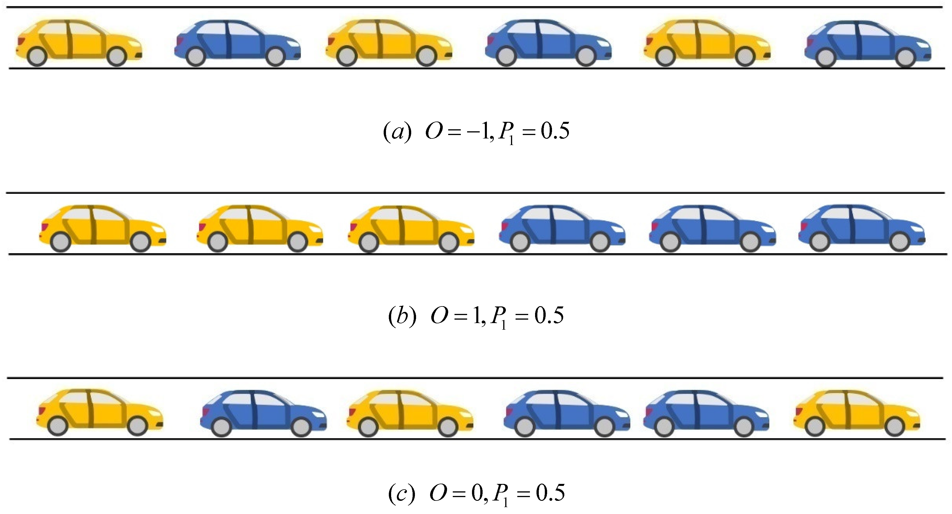
5.2. Experiment 2: Platoon Intensity

Jiang et al. [43] have previously demonstrated that platoon intensity can affect road capacity and that there is a positive correlation between platoon intensity and road capacity. Therefore, this section will explore the impact of different CAV platoon intensities on mixed traffic flow based on the longitudinal control strategy of CAV using TV-MPC. The acceleration of the head vehicle is set as shown in Equation (30), with the remaining experimental settings consistent with those in the previous experiment.

$$\left\{\begin{array}{ll}{a}_0\left(t\right)=0\mathrm{m}/\mathrm{s},& \hspace{0.17em}\mathrm{t}<2\mathrm{s},7<\mathrm{t}<17\mathrm{s},27<\mathrm{t}<32\mathrm{s},37<\mathrm{t}<100\mathrm{s}\\ a_0\left(t\right)=2\mathrm{m}/\mathrm{s},& \hspace{0.17em}2<\mathrm{t}<7\mathrm{s},32<\mathrm{t}<37\mathrm{s}\\ a_0\left(t\right)=-1.5\mathrm{m}/\mathrm{s},& 17<\mathrm{t}<27\mathrm{s}\end{array}\right.$$

(30)

where $a_0\left(t\right)$ is the acceleration of the head vehicle at time $t$.

Figure 6 illustrates the impact of different CAV platoon intensities on the evolution of mixed traffic flow under a CAV penetration rate of 50%. The evaluation metrics include CO₂ emissions, fuel consumption, velocity error, and speed fluctuations. Figure 6a shows the variation in CO₂ emissions under different platoon intensities. The bar chart indicates that CO₂ emissions reach their maximum when the platoon intensity is highest (i.e., CAV and HDVs are completely separated), while CO₂ emissions are minimized when the platoon intensity is negative. Overall, under the same CAV penetration rate, CO₂ emissions increase with higher platoon intensity. By comparing Figure 6a, Figure 6b and Figure 6d, it is evident that CO₂ emissions, fuel consumption, and speed fluctuations exhibit trends highly correlated with platoon intensity. This is because, under the same conditions, speed fluctuations are positively correlated with CO₂ emissions and fuel consumption. Figure 6c demonstrates that the control performance of TV-MPC is also influenced by platoon intensity. A smaller platoon intensity, where CAV and HDVs are more dispersed, not only reduces the risk of multiple consecutive HDVs amplifying disturbances but also allows each CAV to better utilize its ability to smooth oscillations.

In summary, under a fixed CAV penetration rate, the proposed TV-MPC control strategy is more suitable for mixed traffic flow with lower platoon intensity. This finding provides important insights for optimizing CAV distribution in mixed traffic flow and further validates the adaptability and effectiveness of the TV-MPC control strategy across different platoon intensity scenarios.

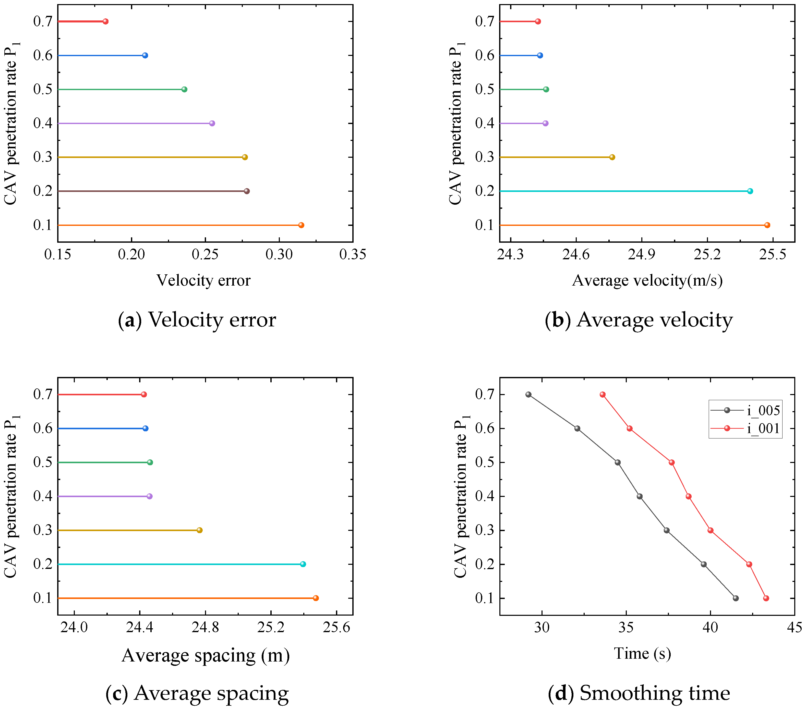
5.3. Experiment 3: CAV Penetration Rates

Existing research indicates that in mixed traffic flow systems, an increase in the penetration rate of CAV contributes to enhancing traffic capacity and accelerating the dissipation of disturbances. Consequently, the subsequent exploration will focus on the impact of different CAV penetration rates on mixed traffic flow based on the TV-MPC strategy proposed in this paper. To facilitate the representation of various CAV penetration rates and considering the real-time computation of the control strategy, the experiment is designed with a mixed platoon consisting of a total of 11 vehicles, including 1 head vehicle and 10 following vehicles. Subsequently, numerical simulations were conducted on mixed platoons with different CAV penetration rates ranging from $P_1=0.1$ to $P_1=0.7$, where CAV are randomly distributed under each distinct penetration rate. The acceleration of the head vehicle can be shown in Equation (31).

$$\left\{\begin{array}{ll}{a}_0\left(t\right)=0\mathrm{m}/\mathrm{s},& \hspace{0.17em}\mathrm{t}<2\mathrm{s},9<\mathrm{t}<14\mathrm{s},19<\mathrm{t}<100\mathrm{s}\\ a_0\left(t\right)=-2\mathrm{m}/\mathrm{s},& \hspace{0.17em}2<\mathrm{t}<9\mathrm{s}\\ a_0\left(t\right)=2\mathrm{m}/\mathrm{s},& 14<\mathrm{t}<19\mathrm{s}\end{array}\right.$$

(31)

To explore the relationship between the efficiency of smoothing oscillation waves and the CAV penetration rate, this paper defines the time required for all vehicles in the mixed platoon to return to an equilibrium state as a measure of the efficiency of the TV-MPC strategy in smoothing oscillation waves, as shown in Equation (32).

$$T_c=\min \left\{t|a_i\left(t\right)\le \varsigma \right\},i\in C\cup H$$

(32)

where $\varsigma$ is the given threshold, we select 0.05 and 0.01 m/s².

Figure 7 sequentially presents the evolution of velocity error, average velocity, average spacing, and smoothing time under CAV penetration rates ranging from 10% to 70%. The results from Figure 7a,c indicate that as the CAV penetration rate increases, both the velocity error and average spacing of the mixed platoon exhibit a downward trend. An intriguing observation is that the rate of decrease in velocity error and average spacing is not entirely consistent with the increase in CAV penetration rate. When $P_1$ increases from 0.2 to 0.3, the reduction in velocity error is limited, while the average spacing between vehicles shows a significant decline. The minimal decrease in velocity error suggests that under these conditions, the control precision of the TV-MPC is only marginally improved, which may be related to the arrangement of CAV and the density of the CAV platoon. The notable reduction in average spacing indicates that increasing the CAV penetration rate from 20% to 30% can significantly enhance road capacity. The results from Figure 7b demonstrate that an increase in CAV penetration rate contributes to reducing congestion and improving traffic efficiency. Figure 7d confirms that an increase in CAV penetration rate can significantly expedite the damping of oscillations.

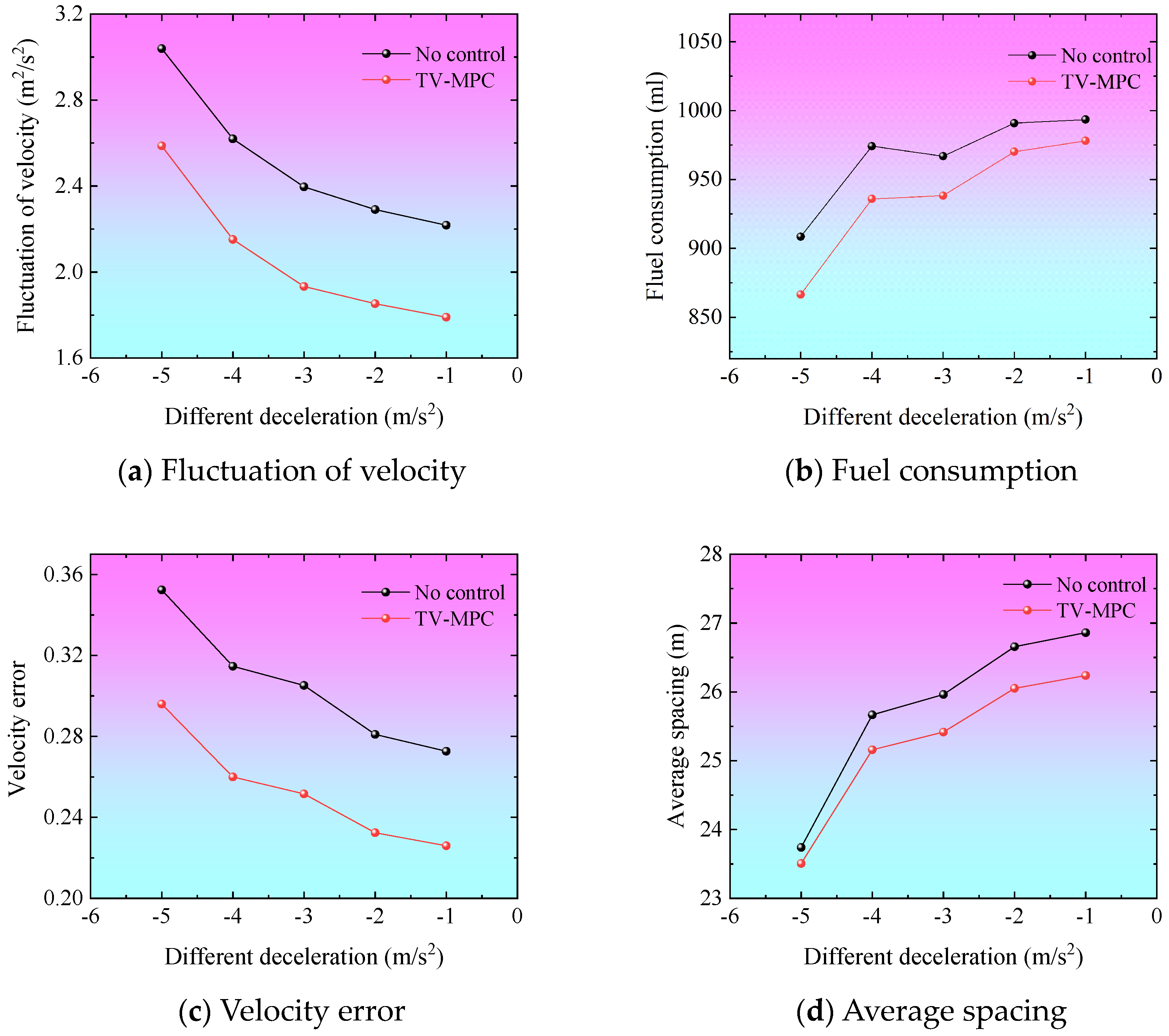
5.4. Experiment 4: Degree of Perturbation

This section analyzes the impact of acceleration changes on mixed traffic flow under the deceleration-constant velocity-acceleration stop-and-go disturbance scenario.

Table 3. Experimental setups for start-stop disturbances.

Order of Actions	Scheme
deceleration- uniform- acceleration	The head vehicle accelerates from V = 15.0 m/s to V = 5.0 m/s with a = −1.0 m/s2, −2.0 m/s2, −3.0 m/s2, −4.0 m/s2, −5.0 m/s2. After driving at a constant velocity for 5 s and then accelerates from V = 5.0 m/s to V = 15.0 m/s with a = 2.0 m/s2.

presents the specific experimental setup for the head vehicle. To enable a more direct comparison of the impact of varying degrees of head vehicle disturbances on mixed traffic flow, this experiment additionally includes an uncontrolled reference group, where all vehicles are HDVs and no CAV are present. And the experimental results are shown in Figure 8.

Figure 8 illustrates the impact of varying degrees of head vehicle disturbances on mixed traffic flow under conditions with and without the implementation of the TV-MPC strategy. As shown in Figure 8a,c, the results indicate that under such disturbances, the velocity fluctuations and velocity errors of the mixed platoon continuously decrease with the increase in disturbance velocity variation, and the trend of change remains consistent between the two scenarios with and without the control strategy. Additionally, observing Figure 8a,c reveals that when the disturbance velocity variation of the head vehicle in the mixed platoon increases, fuel consumption and average spacing tend to decrease instead. It is worth noting that an interesting finding emerges from comparing Figure 8a and Figure 8c: the difference in fuel consumption between the two control methods decreases as the disturbance velocity variation decreases, while the difference in average spacing increases.

6. Suggestion and Application for TV-MPC

(1) Dynamic Adjustment of CAV Deployment Positions

Experimental results indicate that the position of CAV within the platoon significantly impacts their control performance. When a CAV is positioned at index 3 (i.e., slightly forward in the middle of the platoon), it effectively balances disturbance propagation from preceding and following vehicles while maximizing fuel efficiency and traffic flow efficiency. Therefore, in practical traffic management, it is recommended to dynamically optimize CAV deployment positions through the following methods: (1) Real-Time Traffic State Perception: Utilize roadside units (RSUs) and onboard sensor data to monitor traffic density, speed fluctuations, and disturbance propagation characteristics in real time. (2) Adaptive Position Planning Algorithms: Develop reinforcement learning-based dynamic position adjustment algorithms to select the optimal CAV insertion position based on real-time traffic conditions. For example, in congested scenarios, prioritize deploying CAV at key nodes along disturbance propagation paths to mitigate oscillation potential.

(2) Phased Increase in CAV Penetration Rate

Research shows that increasing the CAV penetration rate has a nonlinear impact on mixed traffic flow performance. For instance, when the penetration rate increases from 20% to 30%, the average spacing significantly decreases, but the optimization of velocity error is limited. Therefore, it is recommended to phase the increase in CAV penetration rate: (1) Initial Phase (Penetration Rate < 30%): Focus on optimizing CAV distribution patterns, avoiding concentrated CAV distribution (high platoon intensity), and prioritizing dispersed layouts to reduce the disturbance amplification effect of consecutive HDV queues; (2) Intermediate Phase (Penetration Rate 30%~50%): Combine high-definition maps and collaborative perception technologies to achieve dynamic platoon control of CAV and HDVs, further enhancing traffic capacity; (3) Mature Phase (Penetration Rate > 50%): Leverage V2X systems for global optimization, utilizing the real-time capabilities of TV-MPC to dynamically adjust control parameters for complex traffic scenarios.

(3) Collaborative Optimization of Platoon Intensity and Disturbance Response

Experiments reveal that smaller platoon intensity (dispersed CAV distribution) is more conducive to the performance of the TV-MPC strategy. Therefore, the following collaborative optimization strategies are proposed: (1) Mixed Platoon Rule Design: Implement lane allocation or speed limit policies to enforce alternating distributions of CAV and HDVs, such as adopting a periodic platoon pattern of “1 CAV + 2 HDVs”; (2) Disturbance Sensitivity Grading Control: Dynamically adjust CAV control weights based on different disturbance intensities (e.g., sudden acceleration or deceleration). For example, prioritize reducing velocity errors for following vehicles in high-disturbance scenarios, while focusing on fuel consumption optimization in low-disturbance scenarios.

7. Conclusions and Discussion

7.1. Conclusions

The study investigates the impact of various characteristics of mixed platoons and disturbances on the control performance of TV-MPC through multiple simulation experiments. Initially, the diverse characteristics of mixed vehicle platoons are described using a Markov chain model. Subsequently, a series of experiments based on TV-MPC are conducted to assess the influence of different disturbance characteristics and mixed vehicle platoons on traffic efficiency, traffic oscillations, vehicle fuel consumption, and pollutant emissions in mixed traffic flow. The main conclusions drawn from this study are as follows: (1) There exists an optimal position for CAV in mixed traffic flow that maximizes control performance. (2) As CAV penetration increases, the control performance of TV-MPC gradually improves. (3) For mixed traffic flow under the same CAV penetration rate, smaller CAV platoon intensity (i.e., more dispersed CAV distribution) results in better control performance. (4) The superiority of the TV-MPC control strategy is more pronounced in scenarios with larger disturbance magnitudes.

7.2. Future Work

In future research, there are several exciting directions for expansion. Firstly, the performance of the TV-MPC strategy under abnormal communication conditions has not been explored in this paper. In future studies, it would be beneficial to describe the communication topology using graph structures and then integrate it into the TV-MPC strategy. Secondly, this paper only adopted the exhaust emission calculation method for internal combustion engine vehicles. With the development of automotive electrification, the calculation and conversion methods for carbon emissions from electric vehicles will be further improved. The impact of disturbances on TV-MPC control under multi-energy vehicle combinations can be further explored. Lastly, the research in this paper mainly remains in numerical simulation. In the future, the applicability of the TV-MPC control strategy can be verified by field testing under different traffic scenarios.

References

1. Zhou, F.; Li, X.; Ma, J. Parsimonious shooting heuristic for trajectory design of connected automated traffic part I: Theoretical analysis with generalized time geography. Transp. Res. Part B Methodol. 2017, 95, 394–420. [Google Scholar] [CrossRef]
2. Ji, Q.; Lyu, H.; Yang, H.; Wei, Q.; Cheng, R. Bifurcation control of solid angle car-following model through a time-delay feedback method. J. Zhejiang Univ.-Sci. A 2023, 24, 828–840. [Google Scholar] [CrossRef]
3. Yao, Z.; Wu, Y.; Wang, Y.; Zhao, B.; Jiang, Y. Analysis of the impact of maximum platoon size of CAVs on mixed traffic flow: An analytical and simulation method. Transp. Res. Part C Emerg. Technol. 2023, 147, 103989. [Google Scholar] [CrossRef]
4. Li, J.; Wu, X.; Bai, X.; Liu, Y.; Xu, M. Intelligent Eco-Driving Control for Urban CAVs Using a Model-Based Controller Assisted Deep Reinforcement Learning. IEEE Trans. Intell. Transp. Syst. 2025, 26, 7624–7639. [Google Scholar] [CrossRef]
5. Zeng, T.; Ferdowsi, A.; Semiari, O.; Saad, W.; Hong, C.S. Convergence of communications, control, and machine learning for secure and autonomous vehicle navigation. IEEE Wirel. Commun. 2024, 31, 132–138. [Google Scholar] [CrossRef]
6. Cummins, L.; Sun, Y.; Reynolds, M. Simulating the effectiveness of wave dissipation by FollowerStopper autonomous vehicles. Transp. Res. Part C Emerg. Technol. 2021, 123, 102954. [Google Scholar] [CrossRef]
7. Li, M.; Cao, Z.; Li, Z. A reinforcement learning-based vehicle platoon control strategy for reducing energy consumption in traffic oscillations. IEEE Trans. Neural Netw. Learn. Syst. 2021, 32, 5309–5322. [Google Scholar] [CrossRef]
8. Wang, J.; Zheng, Y.; Dong, J.; Chen, C.; Cai, M.; Li, K.; Xu, Q. Implementation and experimental validation of data-driven predictive control for dissipating stop-and-go waves in mixed traffic. IEEE Internet Things J. 2023, 11, 2327–4662. [Google Scholar] [CrossRef]
9. Wen, J.; Wang, S.; Wu, C.; Xiao, X.; Lyu, N. A longitudinal velocity CF-MPC model for connected and automated vehicle platooning. IEEE Trans. Intell. Transp. Syst. 2022, 24, 6463–6476. [Google Scholar] [CrossRef]
10. Luo, W.; Li, X.; Hu, J.; Hu, W. Modeling and optimization of connected and automated vehicle platooning cooperative control with measurement errors. Sensors 2023, 23, 9006. [Google Scholar] [CrossRef]
11. Li, S.; Zhou, B.; Xu, M. Longitudinal car-following control strategy integrating predictive collision risk. Appl. Math. Model. 2023, 121, 1–20. [Google Scholar] [CrossRef]
12. Lyu, H.; Guo, Y.; Liu, P.; Wang, T. Uncertainty-Aware Dynamics Modeling and Data-Driven Robust Predictive Control for Mixed Vehicle Platoon. IEEE Internet Things J. 2025, 12, 17948–17963. [Google Scholar] [CrossRef]
13. Li, J.; Cheng, R. A real-time adaptive signal control method for multi-intersections in mixed connected vehicle environments. J. Zhejiang Univ.-Sci. A 2025, 1, 189. [Google Scholar]
14. Ding, H.; Wang, L.; Zheng, N.; Cheng, Z.; Zheng, X.; Li, J. A novel hierarchical perimeter control method for road networks considering boundary congestion in a mixed CAV and HV traffic environment. Transp. Res. Part B Methodol. 2025, 195, 103219. [Google Scholar] [CrossRef]
15. Sun, M.; Zhao, W.; Song, G.; Nie, Z.; Han, X.; Liu, Y. DDPG-based decision-making strategy of adaptive cruising for heavy vehicles considering stability. IEEE Access 2020, 8, 59225–59246. [Google Scholar] [CrossRef]
16. Qu, X.; Yu, Y.; Zhou, M.; Lin, C.T.; Wang, X. Jointly dampening traffic oscillations and improving energy consumption with electric, connected and automated vehicles: A reinforcement learning based approach. Appl. Energy 2020, 257, 114030. [Google Scholar] [CrossRef]
17. Wabersich, K.P.; Hewing, L.; Carron, A.; Zeilinger, M.N. Probabilistic model predictive safety certification for learning-based control. IEEE Trans. Autom. Control 2021, 67, 176–188. [Google Scholar] [CrossRef]
18. Wang, J.; Pant, Y.V.; Jiang, Z. Learning-based modeling of human-autonomous vehicle interaction for improved safety in mixed-vehicle platooning control. Transp. Res. Part C Emerg. Technol. 2024, 162, 104600. [Google Scholar] [CrossRef]
19. Shi, H.; Chen, D.; Zheng, N.; Wang, X.; Zhou, Y.; Ran, B. A deep reinforcement learning based distributed control strategy for connected automated vehicles in mixed traffic platoon. Transp. Res. Part C Emerg. Technol. 2023, 148, 104019. [Google Scholar] [CrossRef]
20. Guo, G.; Yue, W. Sampled-data cooperative adaptive cruise control of vehicles with sensor failures. IEEE Trans. Intell. Transp. Syst. 2014, 15, 2404–2418. [Google Scholar] [CrossRef]
21. Akram, M.A.; Liu, P.; Wang, Y.; Qian, J. Gnss positioning accuracy enhancement based on robust statistical mm estimation theory for ground vehicles in challenging environments. Appl. Sci. 2018, 8, 876. [Google Scholar] [CrossRef]
22. Munigety, C.R. A spring-mass-damper system dynamics-based driver-vehicle integrated model for representing heterogeneous traffic. Int. J. Mod. Phys. B 2018, 32, 1850135. [Google Scholar] [CrossRef]
23. Munigety, C.R. Conformity and stability analysis of a modified spring–mass–damper system dynamics-based car-following model. Int. J. Mod. Phys. B 2019, 33, 1950025. [Google Scholar] [CrossRef]
24. Wildhagen, S.; Pezzutto, M.; Schenato, L.; Allgöwer, F. Self-triggered MPC robust to bounded packet loss via a min-max approach. In Proceedings of the 2022 IEEE 61st Conference on Decision and Control (CDC), Cancun, Mexico, 6–9 December 2022; pp. 7670–7675. [Google Scholar]
25. Bongard, J.; Berberich, J.; Köhler, J.; Allgöwer, F. Robust stability analysis of a simple data-driven model predictive control approach. IEEE Trans. Autom. Control 2022, 68, 2625–2637. [Google Scholar] [CrossRef]
26. Wang, Y.; Jin, P.J. Model predictive control policy design, solutions, and stability analysis for longitudinal vehicle control considering shockwave damping. Transp. Res. Part C Emerg. Technol. 2023, 148, 104038. [Google Scholar] [CrossRef]
27. Schwenkel, L.; Köhler, J.; Müller, M.A.; Allgöwer, F. Model predictive control for linear uncertain systems using integral quadratic constraints. IEEE Trans. Autom. Control 2022, 68, 355–368. [Google Scholar] [CrossRef]
28. Schirrer, A.; Haniš, T.; Klaučo, M.; Thormann, S.; Hromčík, M.; Jakubek, S. Safety-extended explicit MPC for autonomous truck platooning on varying road conditions. IFAC-PapersOnLine 2020, 53, 14344–14349. [Google Scholar] [CrossRef]
29. Hu, X.; Xie, L.; Xie, L.; Lu, S.; Xu, W.; Su, H. Distributed model predictive control for vehicle platoon with mixed disturbances and model uncertainties. IEEE Trans. Intell. Transp. Syst. 2022, 23, 17354–17365. [Google Scholar] [CrossRef]
30. Liu, R.; Ren, Y.; Yu, H.; Li, Z.; Jiang, H. Connected and automated vehicle platoon maintenance under communication failures. Veh. Commun. 2022, 35, 100467. [Google Scholar] [CrossRef]
31. Wang, J.; Zheng, Y.; Li, K.; Xu, Q. DeeP-LCC: Data-enabled predictive leading cruise control in mixed traffic flow. IEEE Trans. Control Syst. Technol. 2023, 31, 2760–2776. [Google Scholar] [CrossRef]
32. Talebpour, A.; Mahmassani, H.S. Influence of connected and autonomous vehicles on traffic flow stability and throughput. Transp. Res. Part C Emerg. Technol. 2016, 71, 143–163. [Google Scholar] [CrossRef]
33. Li, L.; Lyu, H.; Wang, T.; Cheng, R. STdi4DMPC: Distributed Model Predictive Control for Connected and Automated Truck Platoon with Mixed Traffic Flow Based on Spatiotemporal Trajectory Prediction. IEEE Trans. Veh. Technol. 2024, 73, 14563. [Google Scholar] [CrossRef]
34. Jiang, Q.; He, B.Y.; Ma, J. Connected automated vehicle impacts in Southern California part-II: VMT, emissions, and equity. Transp. Res. Part D Transp. Environ. 2022, 109, 103381. [Google Scholar] [CrossRef]
35. Liu, M.; Li, Y.; Liu, X.; Chen, Y.; Hao, R. An Integrated Optimization Framework for Connected and Automated Vehicles and Traffic Signals in Urban Networks. Systems 2025, 13, 224. [Google Scholar] [CrossRef]
36. Zong, F.; Yue, S. Carbon emission impacts of longitudinal disturbance on low-penetration connected automated vehicle environments. Transp. Res. Part D Transp. Environ. 2023, 123, 103911. [Google Scholar] [CrossRef]
37. Li, K.; Wang, J.; Zheng, Y. Cooperative formation of autonomous vehicles in mixed traffic flow: Beyond platooning. IEEE Trans. Intell. Transp. Syst. 2022, 23, 15951–15966. [Google Scholar] [CrossRef]
38. Chang, Q.; Chen, H. Enhancing Freeway Traffic Capacity: The Impact of Autonomous Vehicle Platooning Intensity. Appl. Sci. 2024, 14, 1362. [Google Scholar] [CrossRef]
39. Ghiasi, A.; Hussain, O.; Qian, Z.S.; Li, X. A mixed traffic capacity analysis and lane management model for connected automated vehicles: A Markov chain method. Transp. Res. Part B Methodol. 2017, 106, 266–292. [Google Scholar] [CrossRef]
40. Chen, D.; Ahn, S.; Chitturi, M.; Noyce, D.A. Towards vehicle automation: Roadway capacity formulation for traffic mixed with regular and automated vehicles. Transp. Res. Part B Methodol. 2017, 100, 196–221. [Google Scholar] [CrossRef]
41. Jiang, Y.; Sun, S.; Zhu, F.; Wu, Y.; Yao, Z. A mixed capacity analysis and lane management model considering platoon size and intensity of CAVs. Phys. A Stat. Mech. Its Appl. 2023, 615, 128557. [Google Scholar] [CrossRef]
42. Lou, H.; Lyu, H.; Cheng, R. A time-varying driving style oriented model predictive control for smoothing mixed traffic flow. Phys. A Stat. Mech. Its Appl. 2024, 637, 129606. [Google Scholar] [CrossRef]
43. Bowyer, D.P.; Akçelik, R.; Biggs, D.C. Guide to fuel consumption analyses for urban traffic management. Syd. Aust. Aust. Road Res. Board 1984, 21, 485. [Google Scholar]
Figure 1. Schematic of LCC.
Systems 13 00481 g001
Figure 2. Illustrative examples for platooning intensity.
Systems 13 00481 g002
Figure 3. A typical relationship between desired spacing and velocity.
Systems 13 00481 g003
Figure 4. Impact of the CAV in different position.
Systems 13 00481 g004
Figure 5. Fluctuations in velocity under the different position of CAV.
Systems 13 00481 g005
Figure 6. Results for the different platoon intensity with CAV penetration rate P 1 = 0.5 .
Systems 13 00481 g006
Figure 7. Results for the different CAV penetration rates from 0.1 to 0.7.
Systems 13 00481 g007
Figure 8. Results for the different deceleration.
Systems 13 00481 g008