Abstract
Predicting how people choose their travel modes accurately is important in the transportation field. Machine learning (ML) and neural networks (NNs) have gradually become popular in recent years. However, which is better is seldom discussed in previous studies. Therefore, we collect several real-world travel datasets from different countries, and pick five typical ML models, six classic NN models, and ten new NN models for comparison. Some methods for improvement are also considered, including SMOTE, Near-Miss, and using focal loss. The results show that, when looking at the F1-score, the NN models do not perform as well as ML models. While the performances of different classic NN models are similar, making the neural network more complex does not improve the prediction results. Some new NN models can reach the level of ML models on small datasets, but they still perform poorly on large datasets. Due to such a result, we further discuss two important topics: why NN models are not as good as compared to the ones in some other fields, and why this phenomenon is not revealed in many previous papers. In summary, we think this study gives a good reference for future research on predicting travel modes and choosing the right models.
1. Introduction
With rapid urbanization and population growth, urban travel behavior is becoming more complex. Research on travel mode prediction is of great importance: it can help urban planners make better-informed decisions. By grasping travel choice trends, they can allocate resources like roads and public transport facilities more rationally, easing congestion and boosting efficiency. From an environmental perspective, accurate predictions can promote green travel, cutting the transportation sector’s carbon footprint.
From many years ago, the discrete choice model (DCM) [1] became the mainstream tool for the analysis of travel mode choices. Many logit models based on maximum likelihood estimation, e.g., multinomial logit (MNL) [1] and mixed multinomial logit (MMNL) [2] models, have been widely studied. But in recent years, with the rapid development of AI techniques, two new methods have gradually become popular in this field, including machine learning (ML) models and neural network (NN) models [3,4]. Many researchers have found that they are more powerful than DCMs for predicting traffic [5,6,7].
Since both ML models and NN models are popular, a question naturally arises: which one is better? However, this simple question is seldom discussed in the previous papers. Therefore, we want to conduct a systematic comparison between them for travel mode predictions. Firstly, we collect multiple public travel datasets from different countries, including the Netherlands, the UK, and the US. Different sample sizes are considered, ranging from as few as several thousand records to nearly one million records. Next, five typical ML models, six classical NN models, and ten new NN models are chosen for comparison. When focusing on the F1 scores, it is a little surprising that for all the datasets, the performance of NN models is worse than that of ML models. When some typical methods for improvement are used, including SMOTE, Near-Miss, and using focal loss, the situation does not change. Therefore, it is necessary for us to go back to check the details of many previous papers, and try to find the reasons and potential mechanisms. We think such a discussion could be helpful for the future study of this field, including engineering applications.
The rest of this paper is organized as follows. The literature review for this topic is given in Section 2. Section 3 details the various datasets employed in the study. Section 4 presents the main methodology, including the models used, the possible methods for improvement, and the optimizations of model parameters. Section 5 provides the prediction results of various models, and shows a systematic comparison. Section 6 discusses two important questions: Why are these NN models worse? Why is this phenomenon not revealed in many previous studies? Finally, the conclusion is given in Section 7.
2. Literature Review
In this section, we briefly recall the studies about travel mode predictions in recent years, including the approaches with ML models and NN models. Note that we do not use the concept “deep learning” or “deep neural network (DNN)” in this paper, since sometimes it is difficult to say whether a neural network is deep or not. In addition, in some contexts, neural networks are included in broad-sense machine learning. But this paper adopts a narrow definition of machine learning that excludes them.
Firstly, since ML models can automatically find the complex relationships between variables by learning from data instead of making strong assumptions in advance, they have better predictive power than DCMs. For example, Naseri et al. [3] recently emphasized that ensemble learning techniques provide higher accuracy and better interpretability compared to conventional baselines. Li and Kockelman [4] found that the best models for predicting continuous or categorical variables were different, but the average performance of ML models was always better than DCMs. Kashifi et al. [8] claimed that among five ML models, LightGBDT outperformed other models for both under- and over-sampling strategies. Abulibdeh [9] found that XGBoost outperformed other logit models in prediction accuracy, and various trip characteristics significantly influenced mode choices. In the results of Narayanan et al. [10], RF classifier had a slightly higher accuracy than logit models. Similarly, a recent study by Kalantari [11] demonstrated that random forest models consistently outperformed nested logit models across multiple U.S. regions, highlighting the superior predictive power of ensemble learning methods. Le and Teng [5] compared several logit models and two ML models, and claimed all of them can help in predicting the effects of traffic demand management schemes. In addition, by reviewing many articles, Benjdiya et al. [6] found that ML models were more suitable for disaggregate-level analyses, while DCMs were more effective in aggregate-level analyses.
Secondly, inspired by the functions of biological nervous systems, NN models perform very well in many fields, including many transportation-related tasks with complex information. Recently, significant progress has been made in its use for travel mode predictions. For example, Zhang et al. [7], Nam, and Cho [12] proposed a DNN framework for traffic mode choice, which was better than traditional DCMs and simple NN models in prediction accuracy. Wang et al. [13] found DNN outperformed various classical DCMs in both prediction and interpretation, including large sample size and high input dimension, etc. Salas et al. [14] compared five ML/NN classifiers and two DCMs (MNL and MMNL), and found the MMNL model reduced the accuracy gap with ML methods when taste heterogeneity was present. Püschel et al. [15] found that NNs outperformed simultaneous DCMs and the sequential logit model in terms of accuracy and sociodemographic consistency within mobility tool bundles, while the shallow neural network (SNN) was more robust than the deep neural network (DNN). Xia et al. [16] developed an RE-BNN framework by combining the random effect model and Bayesian neural networks. This model outperformed the plain DNN in prediction accuracy. In addition, Wen and Chen [17] proposed a CNN architecture optimized by orthogonal experimental design to predict travel mode choice, and the optimized CNN achieved a very high accuracy.
In addition, we find there are some studies considering the comparisons between various models for travel mode predictions. However, many of them focused on DCMs, and used DCMs as typical benchmarks. In several papers considering the comparison between ML models and NN models, the findings are quite different: some claim that NN models are better [14,17], some others said ML models could be better [7], while in some comparisons the metrics of two types of models are very close [18,19]. Since the focus of some papers tends to be proposing a new model or exploring phenomena in a new dataset, rather than comparing model performance, this topic is usually not explored in depth.
3. Data
In this paper, we concentrate on real datasets rather than synthetic ones. To verify the validity of NN models, we excluded datasets with small sample sizes. We identified three publicly available travel mode choice datasets: MPN from the Netherlands, LPMC from the UK, and NHTS from the US. All datasets used in this study are stated preference (SP) data, which remain a vital tool in recent influential studies for capturing travel behavior shifts [20]. We name them as D1, D2, and D3, and show the details in Table 1. Their sample sizes vary widely, ranging from several thousand to several hundred thousand. Additionally, to obtain datasets of varying sizes, we created subsets (D2A, D3A, and D3B) by selecting the initial records from the original data.

Table 1.
The real datasets studied in this paper.
In all the datasets, there are many available variables, and the dependent variable in this study is always the travel mode. For D2/D2A, there are only four types of travel modes, while for D1 the number of types is eight. But for D3A/D3B/D3, they initially contained 24 different travel modes. After filtering out irrelevant data, the number of travel modes is reduced to 20. These 20 modes are further divided into four main categories: walking, cycling, car, and public transport, which is the same1 as that in D2/D2A. Such a classification also yields two conditions for evaluations, i.e., D3A/D3B/D3-4 (four-class classification) and D3A/D3B/D3-20 (twenty-class classification).
The statistics of the travel modes in these datasets are shown in Figure 1. We can see the following:
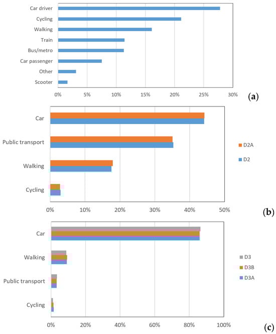
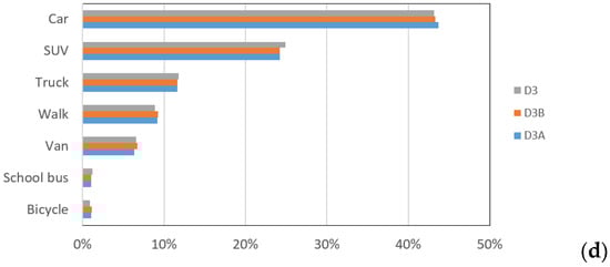
Figure 1.
The distribution of travel mode choices in different datasets. (a) D1, (b) D2, and D2A; (c) D3A/D3B/D3-4; (d) D3A/D3B/D3-20 (only the results greater than 1% are shown).
- (1)
- There are some similarities in these datasets. For instance, the car is consistently the primary choice. Furthermore, the data imbalance in all datasets increases prediction difficulty.
- (2)
- For all the subsets, the proportions of all the travel modes are nearly the same as the original ones. Therefore, the performance differences between the subsets primarily result from the sample size.
- (3)
- Some differences in proportions mainly stem from the differences in typical national conditions. For example, the proportions of cycling in D1 (the Netherlands) are higher than that of walking. However, in D2 (the UK) and D3 (the US), the situation is just the opposite. In addition, the proportions of public transport in D3 (the US) are much lower than that of D1 (the Netherlands) and D2 (UK).
- (4)
- The imbalance is more prominent in D3. In Figure 1d, we only show the seven travel modes with a proportion greater than 1%. In other words, for 13 types in D3A/D3B/D3-20, their proportions are close to zero, and their influence on the final metrics of predictions will be little.
- (5)
- Note that the dependence of travel mode choices upon various variables is a complex topic, which cannot be quickly clarified merely through descriptive statistical charts. For this job, it is better to consider some other approaches, e.g., discrete choice models, which are out of the scope of this paper.
Next, we only consider five main independent variables for each dataset, as shown in Table 2. For D1, the chosen variables are the most important ones mentioned in the brief introduction of MPN. These abbreviations are Dutch words. For both D2 and D3, the chosen variables are age, sex, travel distance, number of family vehicles, and purpose of travel, since they are commonsensically important. The full names of the variables may be not necessarily the same in D2 and D3 (e.g., DISTANCE vs. TRPMILES), but their meanings are. In addition, we can see that in Table 2, the proportional distribution of categorical variables and the statistical results of continuous variables are basically consistent between the complete dataset and the selected subset.
Table 2.
The main independent variables considered for different datasets and their statistics.
Note that these independent variables may not be the best predictors for D2 or D3. However, the primary goal of this study is to compare model performance. Therefore, as long as we use the same independent variables for all the models on each dataset, such a comparison could be fair. In addition, it is possible to consider more variables for D2 or D3. However, we find that after adding several variables, the metrics of all models increase simultaneously, but the final comparative conclusions (e.g., the ranking order of model performance) do not change in any way. Therefore, to ensure consistency across all datasets, we chose to use five variables for the subsequent research.
4. Methodology
4.1. Models Used
In this section, the models used for comparisons are introduced. Firstly, five typical ML models are considered, including LR (logistic regression), KNN (k-nearest neighbors), DT (decision tree), RF (random forrest), and XGB (eXtreme gradient boosting). They have been widely used in many studies introduced in Section 1.
Note that there are some other possible models, but they are not suitable for this study. For example, as discussed in some previous study about machine learning [21], NB (naive Bayes) is a simple model, and its performance is usually not good enough. SVM (support vector machine) is not recommended in this study, since it is very slow, especially when the dataset is large. It takes many hours to obtain the results when running on D3, and it cannot be accelerated by GPU. LGB (light gradient boosting machine) is also popular in recent years. However, its mechanism and performance are usually similar to that of XGB. Therefore, models like NB, SVM, and LGB are not considered in this paper.
Subsequently, we present an overview of the six classic NN models2 utilized in this study:
(1) Multi-Layer Perceptron (MLP for short): It is also known as artificial neural network (ANN), which consists of one or more layers. In this study, two MLP models are considered, namely MLP-1 with one hidden layer, and MLP-2 with two hidden layers (see Figure 2).
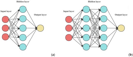
Figure 2.
The structures of MLP models. (a) MLP-1; (b) MLP-2.
(2) One-dimensional Convolutional Neural Network (CNN-1D for short): It is a variant of a convolutional neural network specifically designed to process sequential data, such as time series, text, etc. While travel mode choice data is inherently tabular, its application in this context is justified by transforming the set of input features into a structured, meaningful one-dimensional sequence. The key idea is that the ordering of features is based on their intrinsic logical relationships. For example, we can group features into categories, creating a sequence that starts with personal socio-economic attributes (e.g., age, income, occupation), followed by trip-specific characteristics (e.g., distance, purpose, time of day), and finally environmental factors (e.g., weather, POI density). When a one-dimensional convolutional kernel with a size of three slides along this sequence, it can simultaneously observe three consecutive features and learn their localized interaction patterns. A kernel might, for example, become specialized in recognizing a powerful predictive combination like “high-income, weekday, and morning peak-hour”.
The model structure used in this paper is shown in Figure 3, which is inspired by some classical models, including LeNet and VGG-16. Here, the input tabular data first undergoes feature extraction through one or two one-dimensional convolutional layers, then the data is processed by a flattening layer. Next, it enters a fully connected layer for further feature transformation and processing. The dropout layer is used to prevent overfitting, and finally, the classification result is output through the softmax layer.
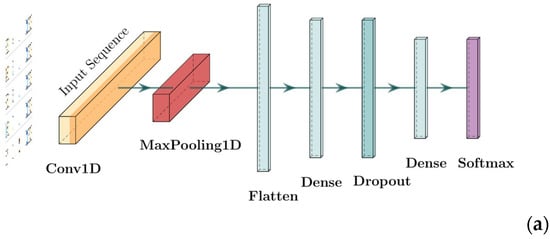
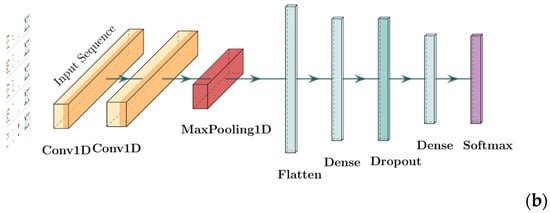
Figure 3.
The structures of CNN-1D models. (a) CNN-1D-1; (b) CNN-1D-2.
(3) Two-dimensional Convolutional Neural Network (CNN-2D for short): It is also a typical form of CNN, and the model structure used in this paper is shown in Figure 4. The application of CNN-2D to tabular data is a more conceptual adaptation, requiring the feature vector to be reshaped into a two-dimensional “feature image” or matrix. For instance, a vector of 16 features can be constructed into a four × four matrix. We arrange the features within this grid to position-related attributes close to each other. For example, one row could represent personal attributes, a second row could represent trip details, and a third could represent land-use characteristics. When a two × two convolutional kernel slides over this ‘feature image’, it can learn high-order patterns that span multiple feature categories simultaneously. For example, one application of the kernel might cover the features [income, car ownership] from the first row and [trip cost, trip purpose] from the second row.
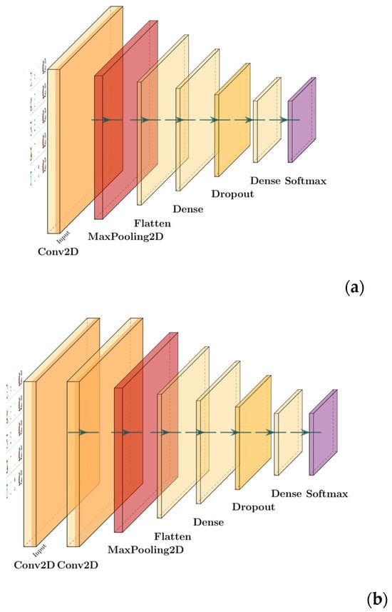
Figure 4.
The structures of CNN-2D models. (a) CNN-2D-1; (b) CNN-2D-2.
Next, for further comparison, we introduce ten new NN models. All of them were recently proposed, and the authors claimed that they were designed for tabular data. They are ResNet [22], SNN [23], AutoInt [24], GrowNet [25], NODE [26], DCN-V2 [27], FT-Transformer [28], TabNet [29], DeepNet [30], and GBDT + DNN [31]. Table 3 summarizes the basic features of the ten models and their specific designs for tabular data.
Table 3.
The basic features of the ten new NN models.
Finally, note that the essence of our study is the classification problem, and the dependent variables in our study are discrete. Therefore, some other typical transport-related models (e.g., STGNNs) are not suitable for this study, since the dependent variables are continuous.
4.2. Possible Methods for Improvement
In order to improve the performance of various models, we also consider three possible methods, including SMOTE, Near-Miss, and using focal loss:
- ▪
- SMOTE (synthetic minority over-sampling technique) is a synthetic minority over-sampling technique [32]. The algorithm flow is as follows:
- (1)
- For each sample x in the minority class, the Euclidean distance is used as the standard to calculate its distance to all the minority class samples, and its k-nearest neighbor is obtained.
- (2)
- A sampling ratio is set according to the sample imbalance ratio to determine the sampling rate N. For each minority sample X, a number of samples are randomly selected from its k-nearest neighbors, assuming that the selected nearest neighbors are Xn.
- (3)
- For each Xn, a new sample is constructed with the original sample according to the following formula:
- ▪
- Near-Miss is an under-sampling technique [33]. It aims to balance the class distribution by randomly eliminating most class examples. The basic intuitions are as follows:
- (1)
- Find the distance between all the majority class instances and minority ones. Here, most classes will be under-sampled.
- (2)
- The noun selects the majority class instance that has the smallest distance from the minority one.
- (3)
- If there are k instances of the minority class, the closest method will result in k × n instances of the majority class.
- (4)
- To find the n closest instances in most classes, there are several variations in the algorithm, including Version 1, Version 2, and Version 3. We selected Version 2 for its superior performance. This version identifies the minority sample that has the greatest distance to the k majority samples.
- ▪
- Focal loss is an innovation loss function for handling imbalanced samples, which was originally proposed by Lin et al. [34] when dealing with object detection. But it is also possible to be used for predictions of travel mode choices. The traditional cross-entropy loss function pays excessive attention to many easy negative samples, which may limit the model performance.
On the contrary, the formula for focal loss is
where pt is the predicted probability of the model for class t, αt is the weight parameter for balancing positive and negative samples, and γ is the focusing parameter. When a sample is correctly classified and pt approaches one, will approach zero. This reduces the contribution of the loss from easy samples. For the difficult samples when pt is small, is relatively larger, and the loss function will pay more attention to these samples.
4.3. Optimization of the Parameters
In this paper, we consider four widely used indicators: Accuracy, Precision, Recall, and F1 score. The formulas are as follows:
where TP, FP, and FN refer to true positive, false positive, and false negative, respectively. The F1 score is a comprehensive metric that contains information about both precision and recall, which is particularly effective for evaluating performance on datasets with imbalanced classes. Thus, in this paper, we choose it as the main indicator for calibrations and comparisons.
Next, we present some examples about how we optimize the model parameters. For the five typical ML models, the typical hyper-parameters considered in this paper are listed in Table 4. Except for some variables that are widely understood in the machine learning community (e.g., n_estimators, max_depth, or learning rate), the meanings of other specific parameters are summarized as follows: For the XGB model, parameters such as gamma, reg_alpha, and reg_lambda are pivotal for regularization and controlling the minimum loss reduction, while subsample and colsample_bytree specify the sampling ratios of training instances and features to prevent overfitting. Regarding the tree-based models (DT and RF), the criterion determines the metric for measuring split quality (i.e., Gini impurity or entropy); specifically for RF, bootstrap indicates whether bootstrap samples are employed during tree construction. In the context of KNN, weights decide if the prediction utilizes uniform voting or distance-based weighting, whereas p sets the power parameter for the Minkowski metric. Finally, as for logistic regression (LR), C refers to the inverse of regularization strength, where smaller values imply stronger regularization.
Table 4.
The dominant hyper-parameters of five typical ML models.
Similarly, the crucial parameters for six classic NN models are shown in Table 5. We do not consider complex networks with even more layers, since we find that increasing the number of layers does not improve model performance, which will be discussed in Section 4.
Table 5.
The dominant hyper-parameters of six classic NN models.
The process of finding the optimal hyper-parameters was conducted through an exhaustive and methodical search. We employed a grid search strategy combined with five-fold cross-validation on the training set. For each model, a grid of possible hyper-parameter combinations was defined based on the search ranges in Table 4 and Table 5. To ensure a rigorous and fair comparison between models, we established a systematic protocol for model training, validation, and testing. For each dataset, we first partitioned the data into three independent sets: a training set (70%), a validation set (15%), and a testing set (15%). During training, we set the maximum number of epochs to 50, which is enough for the losses of all the NN models to be nearly unchanged. Additionally, we employed an early stopping mechanism to prevent overfitting. A dual-layered regularization strategy is also considered. Finally, after evaluating all combinations in the grid, we selected the set of hyper-parameters that yielded the highest average cross-validated F1 score as the optimal configuration.
Here, we show some comparisons between the default values and optimized results in Table 6. This table serves as a typical example, using the D3B-4 dataset, to illustrate the impacts of the hyper-parameter optimization protocol. Generally speaking, the originally effective models (like RF) have little improvement after parameter optimizing. On the contrary, the originally ineffective ones (like KNN or LR) gain more significant improvement, and the differences between default value and optimized value are clearly seen.
Table 6.
Typical examples about the optimization of the model parameters.
Note that there are more parameters in the ten new NN models. The adjustment for them could be very cumbersome and difficult for the users in the field of traffic engineering, which is beyond the scope of this paper. Therefore, for these models, we choose to use the default parameters defined by the authors.
5. Model Results
Firstly, the metrics of all the models are shown in Table 7, Table 8 and Table 9. We find the following:
Table 7.
The averaged metrics of the five ML models. The best F1 scores are marked by red fonts.
Table 8.
The averaged metrics of six classic NN models. The best F1 scores are marked by red fonts.
Table 9.
The averaged metrics of the ten new NN models. The best F1 scores are marked by red fonts.
- (1)
- Generally speaking, when observing the F1 scores, the averaged performance of NN models is worse than ML models, as calculated in Table 10. This situation is not as expected as before, which will be discussed later. For the largest one (D3-20), the maximum F1 score of NN models is even smaller than the minimum value of ML models: 0.147 (GrowNet) < 0.192 (LR).
Table 10. The averaged F1 scores for different types of models. The best F1 scores are marked by red fonts.
- (2)
- Among the five ML models, the performance of RF is the best for large datasets (D3, D3A, and D3B). The main reason is that RF is based on ensemble learning and incorporates random sampling and feature selection mechanisms. This increases the model diversity and makes it more robust against overfitting. However, for smaller datasets, the best choice is not so clear. In addition, LR is always the worst one among the ML models. Such a situation is easy to understand: the linear assumption of LR may lead to limitations when dealing with non-linear data.
- (3)
- The performance of six classic NN models are similar. For all the datasets, the differences between CNN-1D, CNN-2D, and MLP are not significant. This may be because there are no obvious local correlation patterns among the variables involved, or these local correlations are not key factors in this task. In addition, adding layers cannot improve the results for both CNN and MLP. For some situations (e.g., CNN-2D in D3A-20, MLP in D3B-4), the model with one layer could be better than that with two layers. In other words, increasing model complexity is not helpful for such a prediction problem.
- (4)
- The results of the ten new NN models are also unsatisfactory. It seems that they have better performance in a smaller dataset. For example, the best one among them in D1 (ResNet) is at least better than some ML models (LR and DT). However, with the increase in sample number, the advantages of new NN models gradually diminish. As shown in Table 10, in D2A/D2, their performances are similar to classic NN models, while in D3A/D3B/D3, they become even worse.
- (5)
- Differences between the datasets are observed. As introduced in Table 1 and Table 2, the sample sizes of D2 and D3A-4 are nearly the same, and their dependent variables (travel modes) and the five independent variables (age, sex, travel distance, number of family vehicles, and purpose of travel) are also the same. However, the metrics of the same models are different in Table 7, Table 8 and Table 9. For example, most accuracies in D3A-4 are higher than D2, while most F1 scores in D3A-4 are lower. In other words, the internal characteristics of the datasets selected in this paper actually vary significantly. This is also beneficial for us to fully examine and compare the characteristics of various models from different perspectives.
- (6)
- The sizes of datasets are also important. Generally speaking, smaller datasets are easier to predict. In addition, the simple problem with four types is easier than the difficult one with twenty types for all the datasets. This may be because the class imbalance problem is exacerbated in larger datasets, especially in D3.
Note that the results shown in Table 7, Table 8 and Table 9 are the averaged values after running ten times. And we also show the standard deviations of these models in Table 11. Since a similar phenomenon can be found in other datasets, for simplicity, we only show the results of D3B as an example. Here the results of LR, KNN, and XGB are not presented, since they are always zero for this situation. We can see that the randomness of the results of all ML models is very low, since their model structures are simple: they have a limited number of parameters and a highly deterministic training process. On the contrary, the fluctuations in new NN models are more evident, due to their complexity when training. Nevertheless, even when we consider the best of NN models, they are not better than the averaged results of ML models.
Table 11.
The standard deviations of the metrics of some models for D3B.
If we pay attention to some other metrics rather than F1 scores, we can see something new. For example, the precisions of NN models are usually higher than that of ML models, while the recalls of NN models are lower. Therefore, we want to improve the recalls by different means.
As we discussed in Section 3, there are three possible methods, including SMOTE, Near-Miss, and using focal loss. However, they are not only applicable for NN models, but also for ML models. Therefore, we choose to further compare the results of ML models and NN models based on these methods. For simplicity, we only present the typical cases with relatively obvious improvement effects in Table 12, Table 13 and Table 14. We can see the following:
Table 12.
The effect of SMOTE on some models for D3A-20.
Table 13.
The effect of Near-Miss on some models for D2.
Table 14.
The effect of using focal loss on some models for D3B-20.
- (1)
- The improvement in SMOTE is significant for many models. For some models, e.g., XGB and RF, the new F1 score is even more than two times the original value. At the same time, the improvement in F1 score by Near-Miss is also not too bad. Such phenomena coincide with what we can observe in some previous studies.
- (2)
- From Table 12 and Table 13, we can see that all the recalls have been increased, and the values of recalls and precisions have become nearly the same for the same model. Although the mechanisms of SMOTE and Near-Miss are not the same (e.g., the differences between under-sampling and over-sampling), similar results could be obtained, since both methods change the proportional relationship between FP and FN.
- (3)
- On the contrary, the effect of using focal loss is not ideal in Table 14. The marginal improvement can be nearly ignored. This may be because the imbalance in the weights of positive and negative samples is more severe, making it very difficult to find appropriate parameters.
- (4)
- For all the models, the improvement from SMOTE, Near-Miss, or using focal loss does not change the magnitude relationship between the results of ML models and NN models. In other words, regardless of using the conventional method or these improved methods, ML models are always better than NN models, including the new ones proposed in recent years. This conclusion seems a bit counterintuitive, but it is indeed the result after being tested.
Finally, we also show the running time for each model in Table 15. For simplicity, only the results of the smallest and largest datasets are presented. Here, h/m/s means hour/minute/second. The device we used has an Intel Core i7-12700H CPU, 32 GB of memory, and an NVIDIA GeForce RTX 3060 graphics card. It is easy to understand that ML models are always faster than NN models. Nevertheless, the significant differences between their running times further emphasize the deficiencies of NN models, especially when “the ancient model” (e.g., DT) only needs 4 s and “the advanced model” (e.g., a transformer-based model) needs more than 9 h for a large dataset.
Table 15.
The running times of all the models on two datasets.
6. Discussions
Next, after the comparisons between different models based on different datasets, we find that there are two important topics to be discussed:
(1) Why are neural networks not good for travel mode predictions?
In recent years, the effects of neural networks have been proved in many fields, especially in CV, NLP, etc. However, the effects seem unsatisfactory in some other fields, e.g., the predictions for travel mode choices. It is easy to understand that the performance of neural network depends on the amount of data. However, in this paper, we find that the results of both classic and new NN models become even worse when the datasets become larger. For such an unexpected situation, we think the possible explanations are as follows:
- ▪
- The type of input variables. For the travel mode predictions, many input variables are discrete. However, most NN models are typically based on the assumptions of continuity, such as gradient-based optimization methods. When faced with discrete variables, these methods may struggle to find optimal solutions because the discrete nature of the data does not allow for smooth gradients [35]. This makes it difficult for the models to capture complex relationships and patterns hidden within the data [36].
- ▪
- The importance of feature engineering. Typical machine learning models can better adapt to large databases through some traditional feature engineering methods. However, neural networks are restricted by the representation of the original data, and require more complex feature extraction and representation learning processes [37]. Recent studies also confirmed that without massive datasets, advanced gradient boosting models often outperform deep learning architectures on tabular travel data [38]. If the input layer and preprocessing steps of the neural network are not carefully designed (e.g., only five variables are directly input), it may not be able to effectively process this data.
- ▪
- The influence of local features. When the amount of data becomes large, the gradient descent process of the neural network may be inevitably affected by noise or local optimal solutions. This may result in overfitting to the local features of some samples, making its performance decline. In contrast, machine learning models can make better use of the newly added data to enhance generalization ability. For example, RF can construct multiple decision trees by randomly selecting features and samples. It is more robust to noise and local features, and the risk of overfitting can be reduced.
- ▪
- The lack of rotation invariance. As stated in Grinsztajn et al. [36], neural networks have rotation invariance because their learning process does not rely on the direction of features. This characteristic enables neural networks to perform outstandingly when processing data such as images. Since the orientation of an image can be arbitrary, neural networks are still able to recognize the same objects. However, the structured data (like tabular data) generally does not have rotational invariance. For example, each feature in the data of travel mode choice has a fixed position and direction. If they are rotated, the performance of the model will become worse. As a result, the advantages of neural networks cannot be fully utilized when dealing with residents’ travel mode data.
- ▪
- The possibility of overfitting. For some neural networks, especially the new NN models with complex structures, overfitting may be inevitable. Many papers about the new NN models did not mention the total parameter numbers of these models. But as introduced by NODE [26] and TabNet [29], their values could be higher than one million. However, even in the largest dataset of this paper (D3), the sample number is lower than one million. Under such conditions, the advantages of neural networks cannot be brought into play.
Finally, we want to mention that for travel behavior predictions, we cannot completely reject the possibility that there may exist an NN model which is better than ML models. Nevertheless, we find that the existing and commonly used NN models are unable to achieve this goal. At the same time, the design of a new NN model capable of achieving this effect may pose challenges for many users. While such a model may still emerge in the future, using ML models for predictions could be a better choice at present. In addition, in this paper, we only focus on typical tabular data, while some high-dimensional data such as GPS trajectories or image-based modes are not considered. In the future, it is also necessary to study NN superiority boundaries by collecting more data with different forms.
(2) Why are deficiencies of neural networks not revealed in previous studies?
In fact, the comparisons between different models for travel mode predictions are not new. Such a topic has been discussed in some previous papers. However, none of them give the clear conclusion of “ML models are better than NN models” [18,19]. We consider this from several different perspectives:
Firstly, in studies about the ten new models, it is clear that none of them considered datasets about travel behaviors. On the contrary, the datasets used are about users’ ratings on movies [24], rank task about documents [25], simulated physics experiments [28], inverse dynamics of an anthropomorphic robot arm [29], etc. Therefore, the comparative experiments in these articles may not have much reference value for our study. Although the data of travel behaviors also belong to “tabular data”, their features could be different from the datasets in other fields. In other words, simply applying these “models designed for tabular data” may not be a good choice for predicting travel behaviors.
Next, when we focus on the studies about travel behaviors, we find some important aspects:
- ▪
- The object of comparisons: Many previous studies concentrate on the performance of discrete choice models (DCMs), and MNL/BL is usually considered as a typical benchmark. At the same time, some other studies considered different types of logit models. For example, Wang et al. [13], Salas et al. [14] studied the MMNL model when considering heterogeneity. Zhang et al. [7], Le and Teng [5] used the NL model, while Nam and Cho [12], Xia et al. [16], Püschel et al. [15] used both NL and CNL models. Wang et al. [19] studied an additional ten generalized linear models for a comprehensive comparison. Theoretically speaking, it is easy to understand that all of them can obtain the natural conclusion that “ML models are better than DCMs”. This is because the assumption of DCMs about utility norms is too simple and linear, and it has trouble handling categorical explanatory variables. However, this is different from the topic discussed in this paper.
- ▪
- The focus of studies: In many papers considering the comparison between different models, this topic is not the main concern. Instead, the main topic is about the proposal of one or more new models, e.g., DNN-A model in Nam and Cho [12], BMTM-DLP model in Lai et al. [39], RE-BNN model in Xia et al. [16], MTLDNN-M model in Bei et al. [40], “the optimized CNN model” in Wen and Chen [17], and several NN models in Kashifi et al. [8], etc. These authors tried to prove that their new models are better than the selected benchmark models (usually logit models, as mentioned in the last paragraph). In other words, the effects of many machine learning models are not fully considered.
- ▪
- The metrics for evaluations: In many previous studies, the metrics for evaluations differ. Some of them are related to specific problems, e.g., Nam and Cho [12], Le and Teng [5] and Xia et al. [16] chose to study the travel mode shares and their absolute values of errors when predicting. Similarly, Püschel et al. [15] considered the deviation in the predicted distributions. Some others focused on the losses or errors during the training, including Wang et al. [13] and Abulibdeh [9]. Martín–Baos et al. [18] studied some new indicators which were not widely used, e.g., the GMPCA. The only one metric considered by all the studies is accuracy. However, as shown in Table 10, for each dataset, the accuracy of the different models is always similar. If we only look at accuracy, it is too difficult to determine whether NN models are really better.
A similar situation could be observed in other papers and datasets, especially when the papers concentrated on model comparisons (Wang et al. [19]; Martín–Baos et al. [18]). For example, in Figure 2 of Wang et al. [19], the mean accuracy of DNN/RF/Boosting is 57.79/57.05/57.03, while in Table 7 of Martín–Baos et al. [18], that of DNN/RF/XGBoost is 77.23/76.86/78.83. In summary, for travel mode predictions, especially when the sample is imbalanced, we think accuracy is not good enough as a criterion for evaluations.
- ▪
- The size of datasets: In some papers, the metrics of NN models are significantly better than that of ML models, e.g., Wen and Chen [17]. However, since the sample number in this paper is only 1192, we think the “good performance” of NN models may be due to overfitting. Actually, similar situations could be seen in other studies considering more datasets. For example, in Table 4 of Salas et al. [14], when the sample size is 1000, the accuracy of NN model (0.840) is much better than all the ML models (max = 0.730). However, when the size increases to 3000 or 5000, that of NN model declines (0.755) and becomes very close to the other ones (max = 0.748). Therefore, to avoid overfitting, we think it is necessary to choose a dataset that is not too small.
7. Conclusions
In recent years, the application of neural networks has become very popular in many different fields. However, its effectiveness across all fields still need to be evaluated. In this paper, we concentrate on the task of travel mode predictions, and we find something different: in five datasets with different sizes and classification features, the F1 scores of six classic NN models and ten new NN models are always worse than that of the five ML models, including the best and the average results. When considering some methods of improvement, including SMOTE, Near-Miss, and using focal loss, the situation does not change. For running speeds, ML models are also much faster. Given the different classification characteristics of the tested datasets, we think the generality of such a conclusion could be guaranteed.
Next, we try to discuss two important topics: (1) why NN models are not as good as expected; (2) why they are not revealed in many previous studies. For Topic (1), it may be due to the type of input variables, the importance of feature engineering, the influence of local features, the lack of rotation invariance, and the possibility of overfitting. For Topic (2), the first reason is that the development of these new NN models do not consider the datasets of travel behavior. Also, the improvement in the datasets of other tabular data does not lead to better performance when predicting travel mode choices. Next, for the traffic studies, the reasons may include the object of comparisons, the focus of studies, the metrics for evaluations, and the size of datasets, etc. In summary, this study provides an important theoretical basis for future research and engineering applications about travel mode predictions.
Although we have obtained lots of useful findings, a lot more work is still required. Firstly, more datasets are needed. Generally speaking, it is not easy to find suitable travel mode choice datasets with enough large samples. Nevertheless, as time passes, more public datasets could emerge and become beneficial for this field. Secondly, the development of AI technologies is very fast. It is possible that some new NN models with more advanced structures can be better than the current ones, and the current conclusions made in this paper could change in the coming days. For example, better methods for feature engineering could be helpful. In addition, in order to obtain credible results, we only focus on the real datasets in this paper. Whether synthetic datasets are possible to use still needs to be checked in the future. In summary, if we can accomplish all the aforementioned points, we may be able to propose a more comprehensive decision framework for this topic. Naturally, this will undoubtedly require additional efforts in future research.
Author Contributions
Conceptualization, C.-J.J.; methodology, T.Z. and C.-J.J.; software, T.Z.; validation, T.Z. and Y.S.; formal analysis, T.Z. and C.-J.J.; data curation, T.Z.; writing—original draft preparation, T.Z. and C.-J.J.; writing—review and editing, C.-J.J. and Y.S.; visualization, T.Z.; supervision, D.L.; funding acquisition, C.-J.J. and D.L. All authors have read and agreed to the published version of the manuscript.
Funding
This research was funded by the National Natural Science Foundation of China (No. 71801036 and 71971056).
Data Availability Statement
The links for the public datasets used in this paper are: D1: https://github.com/brendadenisse16/Predicting-Travel-Mode-Choices-with-Logistic-Regression-and-SVM (accessed on 23 November 2025); D2: https://www.icevirtuallibrary.com/doi/suppl/10.1680/jsmic.17.00018 (accessed on 23 November 2025); D3: https://nhts.ornl.gov/.
Conflicts of Interest
The authors declare no conflict of interest.
Notes
| 1 | The original names of the travel modes in D2 are not exactly the same as that in D3, e.g., “public transport” vs. “public transit”. Nevertheless, we consider them as the same thing due to the similarities. |
| 2 | Since the classic neural networks used in this study are not very “deep”, we do not use the concept of “DNN” in this paper. In addition, we think the CNN and MLP models used in this paper belong to the scope of “ANN”, but we do not put emphasis on this concept. |
References
- McFadden, D. Conditional Logit Analysis of Qualitative Choice Behavior. In Frontiers in Econometrics; Zarembka, P., Ed.; Academic Press: New York, NY, USA, 1974; pp. 105–142. [Google Scholar]
- McFadden, D.; Train, K.E. Mixed MNL models for discrete response. J. Appl. Econom. 2000, 15, 447–470. [Google Scholar] [CrossRef]
- Naseri, H.; Waygood, E.O.D.; Patterson, Z.; Alousi-Jones, M.; Wang, B. Travel mode choice prediction: Developing new techniques to prioritize variables and interpret black-box machine learning techniques. Transp. Plan. Technol. 2025, 48, 582–605. [Google Scholar] [CrossRef]
- Li, W.; Kockelman, K.M. How does machine learning compare to conventional econometrics for transport data sets? A test of ML versus MLE. Growth Change 2022, 53, 342–376. [Google Scholar] [CrossRef]
- Le, J.; Teng, J. Understanding influencing factors of travel mode choice in urban-suburban travel: A case study in Shanghai. Urban Rail Transit 2023, 9, 127–146. [Google Scholar] [CrossRef] [PubMed]
- Benjdiya, O.; Rouky, N.; Benmoussa, O.; Fri, M. On the use of machine learning techniques and discrete choice models in mode choice analysis. LogForum Sci. J. Logist. 2023, 19, 331–345. [Google Scholar] [CrossRef]
- Zhang, Z.; Ji, C.; Wang, Y.; Yang, Y. A Customized Deep Neural Network Approach to Investigate Travel Mode Choice with Interpretable Utility Information. J. Adv. Transp. 2020, 2020, 5364252. [Google Scholar] [CrossRef]
- Kashifi, M.T.; Al-Rassas, A.M.; Bakar, K.A.; Al-Japairai, K.A.; Jamali, S.S. Predicting the travel mode choice with interpretable machine learning techniques: A comparative study. Travel Behav. Soc. 2022, 29, 279–296. [Google Scholar] [CrossRef]
- Abulibdeh, A. Analysis of mode choice affects from the introduction of Doha Metro using machine learning and statistical analysis. Transp. Res. Interdiscip. Perspect. 2023, 20, 100852. [Google Scholar] [CrossRef]
- Narayanan, S.; Tzenos, P.; Verani, E.; Vlahogianni, E.I. Can Bike-Sharing Reduce Car Use in Alexandroupolis? An Exploration through the Comparison of Discrete Choice and Machine Learning Models. Smart Cities 2023, 6, 1239–1253. [Google Scholar] [CrossRef]
- Kalantari, H.A.; Sabouri, S.; Brewer, S.; Ewing, R.; Tian, G. Machine learning in mode choice prediction as part of MPOs’ regional travel demand models: Is it time for change? Sustainability 2025, 17, 3580. [Google Scholar] [CrossRef]
- Nam, D.; Cho, J. Deep neural network design for modeling individual-level travel mode choice behavior. Sustainability 2020, 12, 7481. [Google Scholar] [CrossRef]
- Wang, S.; Zhao, J.; Lee, D.H. Deep neural networks for choice analysis: A statistical learning theory perspective. Transp. Res. Part B Methodol. 2021, 148, 60–81. [Google Scholar] [CrossRef]
- Salas, P.; Pezoa, R.; Oliveira, L.; Henríquez, G.; Raveau, S. A systematic comparative evaluation of machine learning classifiers and discrete choice models for travel mode choice in the presence of response heterogeneity. Expert Syst. Appl. 2022, 193, 116253. [Google Scholar] [CrossRef]
- Püschel, J.; Regue, R.; Gerike, R.; Nagel, K. Comparison of discrete choice and machine learning models for simultaneous modeling of mobility tool ownership in agent-based travel demand models. Transp. Res. Rec. 2024, 2678, 376–390. [Google Scholar] [CrossRef]
- Xia, Y.; Chen, H.; Zimmermann, R. A random effect bayesian neural network (RE-BNN) for travel mode choice analysis across multiple regions. Travel Behav. Soc. 2023, 30, 118–134. [Google Scholar] [CrossRef]
- Wen, X.; Chen, X. A New Breakthrough in Travel Behavior Modeling Using Deep Learning: A High-Accuracy Prediction Method Based on a CNN. Sustainability 2025, 17, 738. [Google Scholar] [CrossRef]
- Martín-Baos, J.A.; Ros, L.G.; García-García, F.; López-Sánchez, A.D.; Soria-Olivas, E.; Pérez-Bernabeu, E. A prediction and behavioural analysis of machine learning methods for modelling travel mode choice. Transp. Res. Part C Emerg. Technol. 2023, 156, 104318. [Google Scholar] [CrossRef]
- Wang, S.; Kockelman, K.M.; Lemp, J.D. Comparing hundreds of machine learning and discrete choice models for travel demand modeling: An empirical benchmark. Transp. Res. Part B Methodol. 2024, 190, 103061. [Google Scholar] [CrossRef]
- Shahdah, U.E.; Elharoun, M.; Ali, E.K.; Elbany, M.; Elagamy, S.R. Stated preference survey for predicting eco-friendly transportation choices among Mansoura University students. Innov. Infrastruct. Solut. 2025, 10, 180. [Google Scholar] [CrossRef]
- Jin, C.; Luo, Y.; Wu, C.; Song, Y.; Li, D. Exploring the Pedestrian Route Choice Behaviors by Machine Learning Models. Int. J. Geo-Inf. 2024, 13, 146. [Google Scholar] [CrossRef]
- He, K.; Zhang, X.; Ren, S.; Sun, J. Deep Residual Learning for Image Recognition. In Proceedings of the 2016 IEEE Conference on Computer Vision and Pattern Recognition (CVPR), Las Vegas, NV, USA, 27–30 June 2016; pp. 770–778. [Google Scholar]
- Klambauer, G.; Unterthiner, T.; Mayr, A.; Hochreiter, S. Self-Normalizing Neural Networks. In Proceedings of the 31st Conference on Neural Information Processing Systems (NIPS 2017), Long Beach, CA, USA, 4–9 December 2017. [Google Scholar]
- Song, W.; Shi, C.; Xiao, Z.; Wang, Z.; Sun, L.; Rossi, P. AutoInt: Automatic Feature Interaction Learning via Self-Attentive Neural Networks. In Proceedings of the 28th ACM International Conference on Information and Knowledge Management (CIKM ‘19), Beijing, China, 3–7 November 2019; pp. 1161–1170. [Google Scholar]
- Badirli, S.; Tufan, A.; Kask, K.; Can, F.; User, H.B.; Yilmaz, A. Gradient Boosting Neural Networks: GrowNet. arXiv 2020, arXiv:2002.07971. [Google Scholar] [CrossRef]
- Popov, S.; Morozov, S.; Babenko, A. Neural Oblivious Decision Ensembles for Deep Learning on Tabular Data. In Proceedings of the International Conference on Learning Representations (ICLR 2020), Addis Ababa, Ethiopia, 26–30 April 2020. [Google Scholar]
- Wang, R.; Fu, B.; Fu, G.; Wang, M. DCN V2: Improved Deep & Cross Network and Practical Lessons for Web-scale Learning to Rank Systems. In Proceedings of the Web Conference 2021, Ljubljana, Slovenia, 19–23 April 2021; pp. 1785–1797. [Google Scholar]
- Gorishniy, Y.; Rubachev, I.; Gulin, A.; Babenko, A. Revisiting Deep Learning Models for Tabular Data. In Proceedings of the 35th Conference on Neural Information Processing Systems (NeurIPS 2021), Online, 6–14 December 2021. [Google Scholar]
- Arık, S.Ö.; Pfister, T. TabNet: Attentive Interpretable Tabular Learning. In Proceedings of the 35th AAAI Conference on Artificial Intelligence (AAAI-21), Online, 2–9 February 2021; Volume 35, pp. 6679–6687. [Google Scholar]
- Guo, H.; Tang, R.; Ye, Y.; Li, Z.; He, X. DeepFM: A Factorization-Machine based Neural Network for CTR Prediction. arXiv 2017, arXiv:1703.04247. [Google Scholar]
- Yan, J.; Chen, J.; Wang, Q.; Chen, D.Z.; Wu, J. Team up GBDTs and DNNs: Advancing Efficient and Effective Tabular Prediction with Tree-hybrid MLPs. In Proceedings of the 30th ACM SIGKDD Conference on Knowledge Discovery and Data Mining (KDD ‘24), Barcelona, Spain, 25–29 August 2024. [Google Scholar]
- Chawla, N.V.; Bowyer, K.W.; Hall, L.O.; Kegelmeyer, W.P. SMOTE: Synthetic Minority Over-sampling Technique. J. Artif. Intell. Res. 2002, 16, 321–357. [Google Scholar] [CrossRef]
- Zhang, J.; Mani, I. KNN Approach to Unbalanced Data Distributions: A Case Study Involving Information Extraction. In Proceedings of the International Conference on Machine Learning (ICML), Washington, DC, USA, 21–24 August 2003. [Google Scholar]
- Lin, T.Y.; Goyal, P.; Girshick, R.; He, K.; Dollár, P. Focal loss for dense object detection. IEEE Trans. Pattern Anal. Mach. Intell. 2018, 42, 318–327. [Google Scholar] [CrossRef] [PubMed]
- Shwartz-Ziv, R.; Armon, A. Tabular data: Deep learning is not all you need. Inf. Fusion 2022, 81, 84–90. [Google Scholar] [CrossRef]
- Grinsztajn, L.; Oyallon, E.; Varoquaux, G. Why do tree-based models still outperform deep learning on tabular data? arXiv 2022, arXiv:2207.08815. [Google Scholar] [CrossRef]
- Borisov, V.; Leemann, T.; Seßler, K.; Haug, J.; Pawelczyk, M.; Kasneci, G. Deep Neural networks and tabular data: A survey. IEEE Trans. Neural Netw. Learn. Syst. 2024, 35, 7499–7519. [Google Scholar] [CrossRef]
- Banyong, C.; Hantanong, N.; Nanthawong, S.; Se, C.; Wisutwattanasak, P.; Champahom, T.; Ratanavaraha, V.; Jomnonkwao, S. Machine learning-based analysis of travel mode preferences: Neural and boosting model comparison using stated preference data from Thailand’s emerging high-speed rail network. Big Data Cogn. Comput. 2025, 9, 155. [Google Scholar] [CrossRef]
- Lai, Z.; Chen, C.; Wang, Y.; Wang, J.; Xu, Z. Travel mode choice prediction based on personalized recommendation model. IET Intell. Transp. Syst. 2023, 17, 667–677. [Google Scholar] [CrossRef]
- Bei, H.; Liu, J.; Zhang, Y.; Wang, W. Joint prediction of travel mode choice and purpose from travel surveys: A multitask deep learning approach. Travel Behav. Soc. 2023, 33, 100625. [Google Scholar] [CrossRef]
Disclaimer/Publisher’s Note: The statements, opinions and data contained in all publications are solely those of the individual author(s) and contributor(s) and not of MDPI and/or the editor(s). MDPI and/or the editor(s) disclaim responsibility for any injury to people or property resulting from any ideas, methods, instructions or products referred to in the content. |
© 2025 by the authors. Licensee MDPI, Basel, Switzerland. This article is an open access article distributed under the terms and conditions of the Creative Commons Attribution (CC BY) license (https://creativecommons.org/licenses/by/4.0/).