Symbolic Computation to Solving an Irrational Equation on Based Symmetric Polynomials Method

Abstract

In this article, we examine the use of symmetry groups for modeling applied problems through computer symbolic calculus. We consider the problem of solving radical equations symbolically using computer mathematical packages. We propose some methods to obtain a correct analytical solution for this class of equations by means of the Mathcad package. The application of symmetric polynomials is proposed to ensure a correct approach to the solution. Issues on the solvability based on the physical sense of a problem are discussed. Common errors in solving radical equations related to the specificity of the computer usage are analyzed. Provable electrical and geometrical problems are illustrated as example.

1. Introduction

Currently, an indisputable fact is the widespread and ubiquitous use of computer mathematical packages for the modeling of applied problems in any field [1,2]. As a consequence, the question of the correctness of the solutions obtained using these packages is extremely relevant. This issue is especially critical when performing symbolic calculations, where there is the need to obtain an analytical calculation formula with a large number of variable input parameters. Thus, in this work, some cases are illustrated in which the use of embedded algorithms for computer symbolic calculations leads to the appearance of additional extraneous solutions. The numerical validation of all the obtained solutions described by an analytical formula is not feasible. Therefore, it is necessary to develop a method for obtaining the correct symbolic solution using computer mathematical packages, based on mathematical theory. In this article, it is proposed to use some methods based on the theory of symmetric groups [3].

In this paper, we use such a branch of the theory of symmetric groups as symmetric polynomials [4,5]. Symmetric polynomials are used in a wide class of algebraic problems, in the solution of systems of higher order equations, in the solution of irrational equations, for proving identities and inequalities, for factoring, for simplifying algebraic expressions, for extracting roots and for eliminating irrationalities in the denominator [6,7]. In this article, we consider the use of symmetric polynomials for solving a class of algebraic equations, i.e., the irrational equations, namely, a method is developed for obtaining the correct symbolic solution of this class of equations through the use of mathematical packages. The choice of irrational equations is due to the fact that the specificity of the embedded computer algorithms for solving this class of equations more often than others leads to the appearance of extraneous solutions. As an example, an electrical problem is examined using the mathematical package Mathcad [8,9]. This package is very often used for solving applied problems by virtue of its intuitive user interface. In addition, the article discusses techniques for analyzing irrational equations, in order to adapt the method based on symmetric polynomials to some specific cases. These techniques are further illustrated by the example of a graphical geometrical problem about the size of a submarine.

2. The Method of Symmetric Polynomials for Solving Irrational Equations Using Computer Mathematical Packages

2.1. The Core of the Problem of the Extraneous Solutions

Let us demonstrate the essence of the problem of the false solutions to irrational equations when using computer mathematical packages.

Consider an irrational equation with general parameters:

$$\sqrt{a·z+b}+\sqrt{c·z+d}=f$$

(1)

where $z$ is the variable, $a, b,c,d,f$ are real parameters, with $a$ and $c$ not equal to zero at the same time and $f\ge 0$.

By solving symbolically Equation (1) using the standard tools of the mathematical package Mathcad, we obtain two roots (see the listing of the Mathcad program in Figure 1).

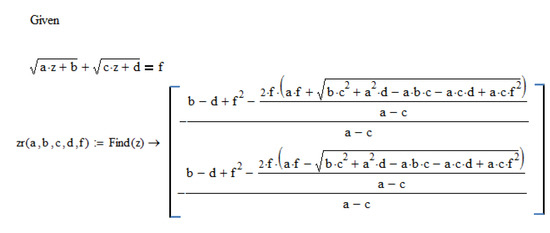
Figure 1. Listing of the Mathcad program for the symbolic solution of Equation (1).

We denote the found roots functions of several parameters as $z_{r1}\left(a,d,c,d,f\right)$ and $z_{r2}\left(a,d,c,d,f\right)$.

Note that the formulas obtained for the roots $z_{r1}\left(a,d,c,d,f\right)$ and $z_{r2}\left(a,d,c,d,f\right)$ do not result in root variants for the case $a=c$, because for $a=c$ Equation (1) has a single root due to the reduction of terms with the same coefficients (see the listing of the program part in Mathcad in Figure 2).

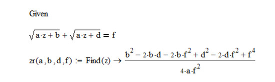
Figure 2. Listing of the Mathcad program for the symbolic solution of Equation (1) if $a=c.$

Similarly, Equation (1) has only one root in the case $a=0$ or $c=0$.

We will consider Equation (1) in the more general case of $a\ne c$.

The analysis of the found roots $z_{r1}\left(a,d,c,d,f\right)$ and $z_{r2}\left(a,d,c,d,f\right)$ shows that they do not satisfy Equation (1) for all the parameter values. To demonstrate this, we introduce the quantities ${∆}_1\left(a,d,c,d,f\right)$ and ${∆}_2\left(a,d,c,d,f\right)$ which are the differences between the left and right sides of Equation (1) where the variable $z$ is substituted with the values of the found roots $z_{r1}\left(a,d,c,d,f\right)$ and $z_{r2}\left(a,d,c,d,f\right),$ respectively. Obviously, if the roots $z_{r1}\left(a,d,c,d,f\right)$ and $z_{r2}\left(a,d,c,d,f\right)$ do satisfy Equation (1), then the values ${∆}_1\left(a,d,c,d,f\right)=0$ and ${∆}_2\left(a,d,c,d,f\right)=0$.

We plot ${∆}_1\left(a,d,c,d,f\right)$ and ${∆}_2\left(a,d,c,d,f\right)$ as functions of the parameter $f$ for $a=2,b=1,c=\pm 4,d=1000$ (see Figure 3a,b).

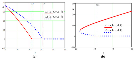
Figure 3. Determining the range of permissible values of the parameter f for Equation (1): (a) c = −4; (b) c = 4.

Figure 3a,b shows that the roots $z_{r1}\left(a,d,c,d,f\right)$ and $z_{r2}\left(a,d,c,d,f\right)$ do not satisfy Equation (1) for all values of the parameter $f$. Therefore, for $c=-4$ (Figure 3a), the root $z_{r1}\left(a,d,c,d,f\right)$ satisfies (1) only for $f\ge 22.4$, and the root $z_{r2}\left(a,d,c,d,f\right)$ satisfies for $f\ge 31.6$. For $c=4$ (Figure 3b), the root $z_{r2}\left(a,d,c,d,f\right)$ satisfies (1) only for $f\ge 31.6$, while the root $z_{r1}\left(a,d,c,d,f\right)$ does not satisfy at all (1).

Thus, using mathematical packages it is possible to ascertain the appearance of extraneous roots in the symbolic solution of an irrational equation of the form (1).

2.2. Methods of Elimination of the False Solutions

The occurrence of extraneous solutions corresponding to certain values of the parameter $f,$ depends on the following fact. The method of solving irrational equations of the type of Equation (1) adopted in the theory of algebra involves the raising of both sides of an equation to the same even degree [10,11]. In this case, the radicals are assumed the principal square root. This occurrence determines the appearance of extraneous roots that correspond to negative values of the radicals, as well as to negative value of the radicands (if we take into account the possibility of complex roots, as implicit in mathematical packages). Two approaches are usually used to eliminate the extraneous roots [10,11].

2.2.1. Validation by the Numerical Solution

The first approach consists in finding all the roots and in their subsequent validation by substitution into the initial equation. This approach is convenient for the numerical solution of equations. In mathematical packages, in particular, in Mathcad, this approach is implemented in the numerical solution of irrational equations, thus ensuring the elimination of extraneous roots. For example, in the numerical solution of Equation (1) for the values of the parameters $a=2, b=1, c=-4, d=1000, f=20$ the result is “No solution”, which corresponds to the plot in Figure 3a (see the listing of the Mathcad program in Figure 4).

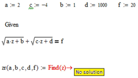
Figure 4. Listing of the program for the numerical solution of Equation (1).

However, when searching for an analytical solution, it is impossible to perform this test of all the roots for all the conceivable values of the parameters. Therefore, when performing symbolic calculations, mathematical packages do not solve this problem at the beginning and, according to the method of raising the two sides of the equation to the same power degree, they provide a calculation formula for the roots (see Figure 1), which includes both positive and negative values of radicals, as well as of the values of the radicands. Therefore, for example, with parameters values given above $a,d,c,d,f$ the value of the first radical in Equation (1) is $\sqrt{z_{r1}\left(a,d,c,d,f\right)·2+1}=22.323$, while the value of the second radical is $\sqrt{z_{r1}\left(a,d,c,d,f\right)·\left(-4\right)+1000}=2.323$. Obviously, the correct sum of the radicals $f=20$ can be obtained by taking the second radical with the negative sign.

2.2.2. Determining the Domain of the Admissible Solutions through Symmetric Polynomials

The second approach for the elimination of the extraneous roots is to solve simultaneously the system given by the irrational equation and by a number of additional inequality constraints imposed on the roots of the equation and arising from the requirement of using only the principal square root. From the above reasoning, it follows that for the problem in question, these will be inequalities that define the range of admissible values of the parameter $f$.

To determine the range of admissible values of the parameter $f$, it was proposed to use the properties of symmetry, namely the properties of symmetric polynomials. In this case, the requirement of symmetry is not imposed on the equation being solved. We use a method for reducing a polynomial to a symmetric form [6]. We introduce the notation:

$$\begin{array}{c}x=\sqrt{a·z+b}, y=\sqrt{c·z+d},\\ {\sigma }_1=x+y, {\sigma }_2=x·y. \end{array}$$

(2)

Obviously the expressions ${\sigma }_1=x+y, {\sigma }_2=x·y$ are the simplest symmetric polynomials. Equation (1) becomes:

$$\begin{array}{c}{\sigma }_1^2=\left(a+c\right)·z+b+d+2·{\sigma }_2,\\ {\sigma }_1=f,\end{array}$$

(3)

from this it derives:

$${\sigma }_2=\frac{f^{2 }-\left(a+c\right)·z-b-d}{2}.$$

(4)

Because the radicals must be non-negative, ${\sigma }_1\ge 0$ and ${\sigma }_2\ge 0$.

Since ${\sigma }_1=f,$ that requirement ${\sigma }_1\ge 0$ is verified for $f\ge 0$.

From the condition ${\sigma }_2\ge 0,$ it follows the range of admissible values for the parameter $f$:

$$f\ge \sqrt{\left(a+c\right)·z+b+d}.$$

(5)

Finally, we solve the system given by Equation (1) and inequality (5):

$$\begin{array}{c}\sqrt{a·z+b}+\sqrt{c·z+d}=f,\\ f\ge \sqrt{\left(a+c\right)·z+b+d}.\end{array}$$

(6)

The consideration of system (6) instead of Equation (1) makes it possible to obtain a symbolic solution without extraneous roots, as we will show on some applied problems.

Note that system (6) corresponds to a generally accepted scheme for setting the range of admissible values when solving an algebraic equation [4,5]. However, in our case, it is not possible to determine the admissible region of the parameter (5) based only on the general form of the initial Equation (1), since it is required the use of symmetric polynomials.

2.3. Application of the Proposed Method for Solving an Electrical Problem

Let us clarify the core of the problem of the extraneous solutions by an example of an applied electrical problem. It is requested to find the optimal distribution of the total power $P=P_1+P_2$ to two users of capacities $P_1$ and $P_2$ with a required total voltage $U=U_1+U_2,$ less than the breakdown voltage. Users resistances are equal respectively to $R_1$ and $R_2$.

According to the theory of electrical circuits, the expressions for the powers are described by the formulas [12]:

$$P_1=\frac{U_1^2}{R_1}, P_2=\frac{U_2^2}{R_2}.$$

(7)

Then, setting as parameters the resistances $R_1$ and $R_2$, the total voltage $U$ and the total power $P$, an irrational equation is derived for the sought variable $P_1$:

$$\sqrt{P_1·R_1}+\sqrt{\left(P-P_1\right)·R_2}=U.$$

(8)

By solving symbolically Equation (8) using the standard tools of the mathematical package Mathcad, we obtain two roots (see the listing of the Mathcad program in Figure 5).

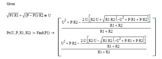
Figure 5. Listing of the Mathcad program for the symbolic solution of Equation (8).

It could be noted that by executing the calculations using the Mathematica or the Matlab packages, equivalent roots are obtained (see the listings of programs in Wolfram Mathematica [13] and Matlab [14,15] packages in Figure 6).

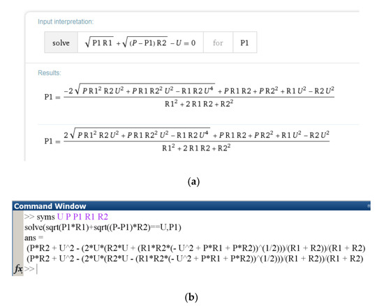
Figure 6. Listings of the programs for the symbolic solution of Equation (2) with the packages: (a) Wolfram Mathematica; (b) Matlab.

The found roots are functions of several parameters $P_{r1}\left(U,P,R_1,R_2\right)$ and $P_{r2}\left(U,P,R_1,R_2\right)$.

After assigning to the parameters the following values $P=8000, R_1=1 ,R_2=2$, the roots of Equation (8) $P_{r1}\left(U,8000, 1,2\right)$ and $P_{r2}\left(U,8000, 1,2\right)$ are plotted as function of the required total voltage $U$ (Figure 7).

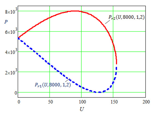
Figure 7. The initial set of the solutions of Equation (8).

Let us verify whether the functions $P_{r1}\left(U,8000, 1, 2\right)$ and $P_{r2}\left(U,8000, 1, 2\right)$ are actually solutions of Equation (8) for any value of $U$. In order to do this, we build a plot of the right side of Equation (8)—simply $Y\left(U\right)=U$, and a plot of the left side of Equation (8), by substituting in it the functions $P_{r1}\left(U,8000, 1, 2\right)$ and $P_{r2}\left(U,8000, 1, 2\right)$ instead of the sought variable $P_1$ (Figure 8). Obviously the solutions $P_{r1}\left(U,8000, 1, 2\right)$ and $P_{r2}\left(U,8000, 1, 2\right)$ are true solutions of the problem only for those values of $U$, where the plots of the left and right sides match.

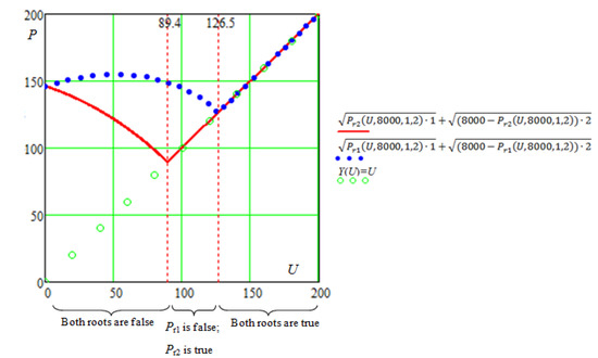
Figure 8. Determining the range of admissible values of the parameter for Equation (8).

According to the plot:

• For U < 89.4 both solutions P_r1 (U, 8000, 1, 2) and P_r2 (U, 8000, 1, 2) are false;
• For 89.4 ≤ U < 126.5 solution P_r1 (U, 8000, 1, 2) is false, while P_r2 (U, 8000, 1, 2) is true;
• For U ≥ 126.5 both solutions P_r1 (U, 8000, 1, 2) and P_r2 (U, 8000, 1, 2) are true.

Thus, we have ascertained that the solution of Equation (8) shown in Figure 5 includes extraneous roots.

2.3.1. Implementation of the Proposed Method

We use the proposed method for the elimination of the extraneous roots. We need to determine the inequalities that define the range of admissible values of the parameter—total voltage $U$.

To determine the range of admissible values of the parameter $U$, it was proposed to use the properties of symmetric polynomials. Note that the Equation (8) here considered is not symmetric with respect to variables $P_1, P_2$. So the plots of the roots $P_{r1}\left(U,8000, 1, 2\right)$ and $P_{r2}\left(U,8000, 1, 2\right)$ are also not symmetric (Figure 7). We introduce the notation:

$$\begin{array}{c}x=\sqrt{P_1·R_1}, y=\sqrt{\left(P-P_1\right)·R_2},\\ {\sigma }_1=x+y, {\sigma }_2=x·y. \end{array}$$

(9)

Equation (8) becomes:

$$\begin{array}{c}{\sigma }_1^2=P·R_2+\left(R_1-R_2\right)·P_1+2·{\sigma }_2,\\ {\sigma }_1=U,\end{array}$$

(10)

from this it derives:

$${\sigma }_2=\frac{U^{2 }-P·R_2-\left(R_1-R_2\right)·P_1}{2}.$$

(11)

Because the radicals must be non-negative, ${\sigma }_1\ge 0$ and ${\sigma }_2\ge 0$.

Since ${\sigma }_1=U,$ that requirement ${\sigma }_1\ge 0$ is verified for $U\ge 0$.

From the condition ${\sigma }_2\ge 0,$ it follows the range of admissible values for the parameter $U$:

$$U\ge \sqrt{P·R_2+\left(R_1-R_2\right)·P_1}.$$

(12)

Comparing the plots of the roots in Figure 8 and the plot of the function ${\sigma }_2\left(U\right)$ in Figure 9 for specific values of $P, R_1, R_2, P_1$, we notice that the lower bound for the value of $U=89.4$ corresponds to the minimum admissible value of the variable $P_1=0,$ while the point of appearance of the second root $U=126.5$ corresponds to the maximum admissible value $P_1=P=8000$.

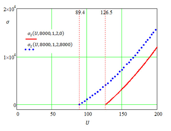
Figure 9. Plot of the function ${\sigma }_2\left(U\right)$.

Finally, we solve the system given by Equation (8) and inequality (12):

$$\begin{array}{c}\sqrt{P_1·R_1}+\sqrt{\left(P-P_1\right)·R_2}=U,\\ U\ge \sqrt{P·R_2+\left(R_1-R_2\right)·P_1}.\end{array}$$

(13)

The plot of the correct analytical solution obtained using Mathcad is shown in Figure 10. Comparing it with the plot in Figure 7, we see that the extraneous roots are eliminated, and, as noted earlier, in the interval $89.4\le U<126.5$ Equation (8) has only one root $P_r\left(U,8000, 1, 2\right)$, while in the interval $U\ge 126.5$—two roots $P_{r1}\left(U,8000, 1, 2\right)$ and $P_{r2}\left(U,8000, 1, 2\right)$.

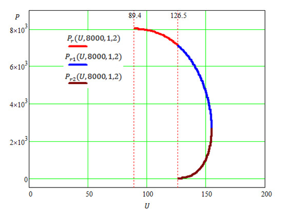
Figure 10. The set of the correct solutions of Equation (8).

2.3.2. A Special Case

Let us consider a special case of Equation (8), when the user resistances are equal $R_1=R_2$. In this case, the left side of Equation (8) is already initially a symmetric polynomial with respect to the variables $P_1, P_2$:

$$\sqrt{P_1·R_1}+\sqrt{\left(P-P_1\right)·R_1}=U.$$

(14)

The plots of the solution (14), shown in Figure 11 and similar to the plots in Figure 7, have a symmetric appearance.

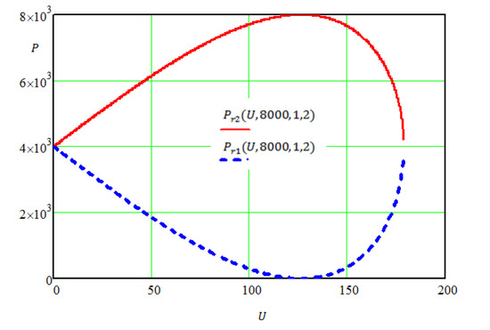
Figure 11. The initial set of the solutions of Equation (14).

System (13) in this case reduces to the form:

$$\sqrt{P_1·R_1}+\sqrt{\left(P-P_1\right)·R_1}=U,U\ge \sqrt{P·R_1}.$$

(15)

The overall form of the analytical solution of system (15), obtained using Mathcad, is shown in Figure 12. The analytical solution is written by using the conditional if operator, which allows to determine a different type of solution for different ranges of values $U$.

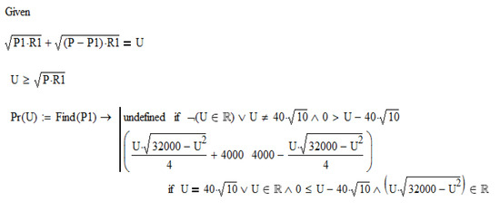
Figure 12. Listing of the program for the symbolic solution of system (15).

The plot of the correct analytical solution of the system (15), shown in Figure 13, has obviously a symmetric appearance, i.e., on the entire allowable interval $U\ge 126.5$ there are two symmetric roots $P_{r1}\left(U,8000, 1, 2\right)$ and $P_{r2}\left(U,8000, 1, 2\right)$.

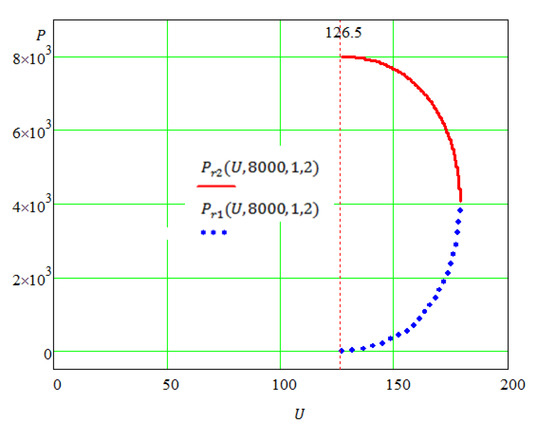
Figure 13. Set of the correct solutions of system (15).

Thus, in this section, we have described a method for obtaining the correct analytical solution of an irrational equation using the properties of symmetry, demonstrating it using as example the solution of Equation (8).

3. Application of Additional Methods of Analysis for Solving Irrational Equations Using Computer Mathematical Packages

In many applications, it is possible to simplify the method of obtaining the correct analytical solution of an irrational equation, if in the process of reduction to a symmetric form, the initial irrational equation is analyzed.

Let us consider the problem of finding the geometrical dimensions of a submarine, whose shape consists of a straight circular cylinder and two identical straight circular cones (Figure 14).

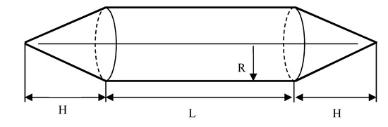
Figure 14. Geometrical dimensions of a submarine.

The surface area $S$ and the volume $V$ of the vessel are given. It is necessary to find the length $L$ of the cylinder, the radius $R$ of the base of the two cones and of the cylinder and the height $H$ of the two cones.

3.1. Initial Formulation of the Problem

According to the known geometry formulas, the surface area and the volume are determined by the following relations [16]:

$$\begin{array}{c}S=2·\pi ·R·\left(L+\sqrt{H^2+R^2}\right),\\ V=\pi ·R^2·\left(L+\frac{2}{3}H\right).\end{array}$$

(16)

Expressing the variable $L$ through both Equation (16), we obtain the relations:

$$\begin{array}{c}{L}_S\left(R,S,H\right)=\frac{S-2·\pi ·R·\left(\sqrt{H^2+R^2}\right)}{2·\pi ·R},\\ L_V\left(R,V,H\right)=\frac{V-\frac{2·\pi ·H·R^2}{3}}{\pi ·R^2}.\end{array}$$

(17)

Equating the ratios

$$L_S\left(R,S,H\right)=L_V\left(R,V,H\right),$$

(18)

we obtain an equation in two variables $H$ and $R$. Considering as parameters the values of $S$, $V$, $R$, we could solve Equation (18) with respect to the variable $H\left(R,V,S\right)$.

3.2. Solution of the Problem in the Initial Formulation

3.2.1. Analytical Solution

As in the previous example (Figure 5), the analytical solution of the irrational Equation (18) in the Mathcad package consists of two roots (see listing in Figure 15).

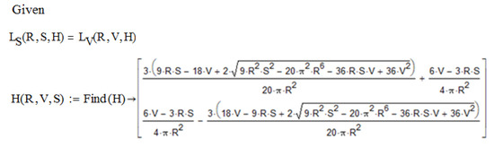
Figure 15. Listing for the solution of Equation (18).

The plots of the roots $H_1\left(R,V,S\right)$ and $H_2\left(R,V,S\right)$ with some specified values for the parameters $S=1000 {\mathsf{м}}^2$ and $V=1500 {\mathsf{м}}^2$ are shown in Figure 16. For the generality of the considered example, we will not yet take into account the physical meaning of the variable $H\left(R,V,S\right)$, allowing for negative and even complex values.

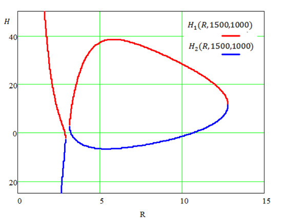
Figure 16. Initial set of the solutions of Equation (18).

3.2.2. Analysis of the Solution of the Problem in the Initial Formulation

Let us check whether the functions $H_1\left(R,1500,1000\right)$ and $H_2\left(R,1500,1000\right)$ are solutions of Equation (18) for all the values of the parameter $R$. In order to do this check, we construct the plots of the left $L_S$ and right $L_V$ sides of Equation (18) with the sought variable $H$ substituted by the functions $H_1\left(R,1500,1000\right)$ and $H_2\left(R,1500,1000\right)$ (Figure 17). Obviously, the solutions are true only for those values of $R$, where the plots of the left and right sides coincide.

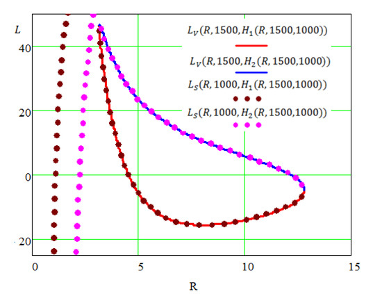
Figure 17. Determination of the range of the permissible values of the parameter for Equation (18).

As can be seen from the plots in Figure 17, the solutions $H_1\left(R,1500,1000\right)$ and $H_2\left(R,1500,1000\right)$ are not valid for some values of $R$, that is, the resulting analytical solution contains extraneous roots (these are the left branches in Figure 16). It is difficult to determine the lower limit of the values of the $R$ parameter so that the solutions are true, because the plots (Figure 16 and Figure 17) show only real values of the roots $H_1\left(R,1500,1000\right)$ and $H_2\left(R,1500,1000\right)$. In this case, generally speaking, the analytical solution presented in Figure 16 includes complex values. This is due to the fact that if the initially real numerical parameters of the equation are not specified in the mathematical package, the symbolic solution is performed over the entire field of the complex numbers. Therefore, for example, when $R=3$, we get the imaginary root $H_1\left(R,V,S\right)=4.025 i$, which satisfies Equation (18), that is, the values of $L_V$ and $L_S$ are complex and coincide.

3.3. Problem Solution Based on Symmetric Polynomials

3.3.1. Determining the Range of Admissible Solutions

In order to determine the range of admissible values for the parameter $R$ of Equation (18), we use also the reduction method to symmetric polynomials. We note that after introducing a restriction for the variable $R$ in the region of the real numbers, we thus proceed to solve the equation in the real domain, and the sought analytical solution will no longer contain complex values.

Transform Equation (18) to the form:

$$3·R·S-6·V-6·\pi ·R^2·\sqrt{H^2+R^2}+4·\pi ·H·R^2=0.$$

(19)

In order to bring the left side of Equation (19) to a symmetric form, it is necessary to introduce a second irrationality of the variable $H.$

For the generality of the considered case we allow negative values of the variable $H ,$ neglecting for the time the physical sense. Therefore, we will consider the two options: $H\ge 0$ and $H<0$.

For $H\ge 0$ Equation (19) can be rewritten in the form:

$$2·\sqrt{H^2}-3·\sqrt{H^2+R^2}=\frac{6·V-3·R·S}{2·\pi ·R^2},$$

(20)

The left side of (20) is not symmetric, however, we select the symmetric part in it and analyze the resulting equation:

$$\left(2·\sqrt{H^2}-2·\sqrt{H^2+R^2}\right)-\sqrt{H^2+R^2}=\frac{6·V-3·R·S}{2·\pi ·R^2}.$$

(21)

Since the values of all radicals in (21) must be non-negative, it follows the inequality:

$$2·\sqrt{H^2}-2·\sqrt{H^2+R^2}<0.$$

(22)

Consequently, the entire left side of Equation (21) is also negative, which implies the negativity of the right side (21):

$$\frac{6·V-3·R·S}{2·\pi ·R^2}<0.$$

(23)

Analogously for $H<0$ Equation (19) can be rewritten in the form:

$$-2·\sqrt{H^2}-3·\sqrt{H^2+R^2}=\frac{6·V-3·R·S}{2·\pi ·R^2}.$$

(24)

In this case, even without isolating the symmetric part, it is obvious that the left side of Equation (24) is negative due to the use of the principal square root. Therefore, for $H<0$ also (17) is true.

Thus, by analyzing Equation (19), we obtain an inequality that determines the range of admissible values of the parameter $R$, which follows directly from (23):

$$R>\frac{2·V}{S}.$$

(25)

Now, by solving the system given by Equation (18) and inequality (25):

$$\begin{array}{c}{L}_S\left(R,S,H\right)=L_V\left(R,V,H\right),\\ R>\frac{2·V}{S},\end{array}$$

(26)

we get the correct analytical solution of Equation (18) without extraneous roots. The general view of the correct analytical solution obtained with Mathcad is exactly identical to the solution presented in Figure 18. Figure 18a shows the plots of the true analytical solution. Figure 18b shows the plots of the left $L_S$ and right $L_V$ sides of Equation (18) with the correct functions $H_1\left(R,1500,1000\right)$ and $H_2\left(R,1500,1000\right)$ substituted in place of the sought variable $H$. Comparing Figure 18a with Figure 16 and Figure 18b with Figure 17, we see that the false solutions were eliminated.

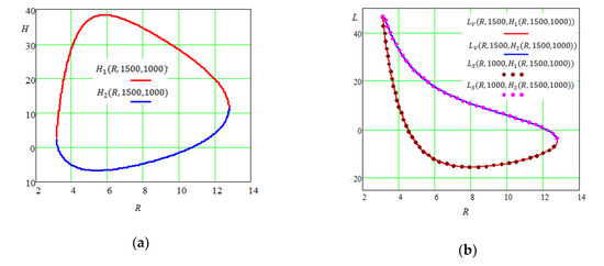
Figure 18. The correct set of the solutions of Equation (18): (a) solutions $H\left(R,V,S\right)$; (b) values of $L_S\left(R,S,H\right)=L_V\left(R,V,H\right)$ corresponding to the solutions.

3.3.2. Eliminating Solutions without Physical Meaning

Now let’s return to the physical meaning of the geometrical problem under consideration. It is necessary to take into account the positivity of the sought values of $H,L,R$. The positivity of $R$ follows from inequality (25). Therefore, it is sufficient to add to system (26) the corresponding inequalities for the quantities $H,L$ using (17):

$$\begin{array}{c}H>0,\\ L_V\left(R,V,H\right)=\frac{V-\frac{2·\pi ·H·R^2}{3}}{\pi ·R^2}>0\end{array}$$

(27)

or

$$\begin{array}{c}H>0,\\ V>\frac{2·\pi ·H·R^2}{3}.\end{array}$$

(28)

Then, solving together (26) and (28), we obtain the correct analytical solution that takes into account the physical meaning of the geometrical quantities. The solutions $H\left(R,V,S\right)$ together with the corresponding values $L_S\left(R,S,H\right)=L_V\left(R,V,H\right)$ are shown in Figure 19. Obviously, they are non-negative sub-regions of the solutions shown in Figure 18.

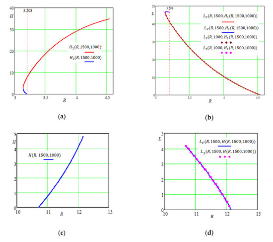
Figure 19. The set of the correct solutions of Equation (18), taking into account the physical meaning: (a) first subdomain of solutions $H\left(R,V,S\right)$; (b) values of $L_S\left(R,S,H\right)=L_V\left(R,V,H\right)$, corresponding to the first subdomain; (c) the second subdomain of the solutions $H\left(R,V,S\right)$; (d) values of $L_S\left(R,S,H\right)=L_V\left(R,V,H\right)$ corresponding to the second subdomain.

It is possible to define up to third digit the boundaries of the first sub-region of solutions as $3.146\le R\le 4.578$, and with $3.146\le R<3.208$ there are two roots $H_1\left(R,1500,1000\right)$ and $H_2\left(R,1500,1000\right)$, while with $R\ge 3.208$ only one $H_1\left(R,1500,1000\right)$. The second subdomain of the solutions is defined for $10.708\le R\le 12.157$, and here there is only one root $H\left(R,1500,1000\right)$.

The corresponding 3d-plot of the solution area $\left(H,L,R\right)$, calculated analytically taking into account the physical meaning of the variables, is shown in Figure 20.

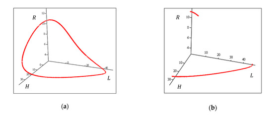
Figure 20. A 3d-plot of the solution area $\left(H,L,R\right)$: (a) region of the correct solutions; (b) region of the solutions with physical meaning.

4. Discussions of the Results

The results obtained in the article give the opportunity to indicate the directions of further research in the field of identified problems.

Primarily, it is necessary to determine the usage field of the proposed method, i.e., the determination of the irrational equations that, can be reduced to a form that allows the use of such a method. The starting point of the study can be the statement [4,5], that there is an asymmetric (globally) polynomial $\overline{F}\left({\sigma }_1,{\sigma }_2\right)$, such as:

$$F\left(x,y\right)=\overline{F}\left(x+y,xy\right),$$

(29)

for any symmetric polynomial $F\left(x, y\right)$.

This problem contains the need of research of method usage possibility for irrational equations with high degree radicals using symmetric polynomials of the form $S_n=x^n+y^n$. This can be realized due to the statement [4,5], that any sum of power $S_n$ is representable as a polynomial in variables ${\sigma }_1=x+y, {\sigma }_2=x·y$. Certainly, this will require additional analysis of the inequalities for the determination of the admissible region of parameter values.

Since one of the main applications of symmetric polynomials in algebra is their use for solving systems of equations [6,7], an extension of the proposed method for solving systems of irrational equations seems to be a promising direction.

A separate study requires the application of the method for system of irrational equations, nonlinear in the variables. In Section 3 of the article, we considered a special case of applying the method for nonlinear irrational equation. However, a generalization of the issue requires additional research, which we plan to conduct in future research.

5. Conclusions

The article presented critical errors in the symbolic solution of irrational equations using mathematical packages. A method of obtaining a correct analytical solution using the properties of symmetry, namely symmetric polynomials, is proposed. Some methods of further analysis of irrational equations with the aim of obtaining a correct analytical solution are presented. The solution methods are established by taking into account the physical meaning of the problems. This algorithm can also be used in innovative engineering education [17], in STEM (Science, Technology, Engineering and Math including Computer Science) education [18].

References

- Fre, P.G.; Fedotov, A. Groups and Manifolds: Lectures for Physicists with Examples in Mathematica; Walter de Gruyter: Berlin, Germany, 2018; 475p. [Google Scholar]
- Brenner, A.; Shacham, M.; Cutlip, B. Applications of mathematical software packages for modeling and simulations in environmental engineering education. Environ. Model. Softw. 2005, 20, 1307–1313. [Google Scholar] [CrossRef]
- Steeb, W.-H.; Tanski, I.; Hardy, Y. Problems and Solutions for Groups, Lie Groups, Lie Algebras with Applications; World Scientific Publishing Company: Singapore, 2012. [Google Scholar] [CrossRef]
- Meier, J.; Smith, D. Algebra and symmetry. In Exploring Mathematics: An Engaging Introduction to Proof (Cambridge Mathematical Textbooks); Cambridge University Press: Cambridge, MA, USA, 2017; pp. 229–249. [Google Scholar] [CrossRef]
- Goodman, F.M. Algebra: Abstract and Concrete; SemiSimple Press: Iowa City, IA, USA, 2015. [Google Scholar]
- Kuang, Y.; Zheng, Y.; Åström, K. Partial Symmetry in Polynomial Systems and Its Applications in Computer Vision. In Proceedings of the IEEE Computer Society Conference on Computer Vision and Pattern Recognition, Columbus, OH, USA, 23–28 June 2014; pp. 438–445. [Google Scholar] [CrossRef]
- Larsson, V.; Åström, K. Uncovering Symmetries in Polynomial Systems. In Proceedings of the 14th European Conference Computer Vision—ECCV 2016, Amsterdam, The Netherlands, 11–14 October 2016; Part III. pp. 252–267. [Google Scholar] [CrossRef]
- Maxfield, B. Essential Mathcad for Engineering, Science, and Math ISE, 2nd ed.; Academic Press: Cambridge, MA, USA, 2009. [Google Scholar]
- Maxfield, B. Essential PTC Mathcad Prime 3.0. A Guide for New and Current Users; Academic Press: Cambridge, MA, USA, 2013; 584p. [Google Scholar] [CrossRef]
- Dugopolski, M. Elementary and Intermediate Algebra, 4th ed.; McGraw-Hill: New York, NY, USA, 2012; 1104p. [Google Scholar]
- Aufmann, R.N.; Barker, V.N.; Lockwood, J. Algebra: Introductory and Intermediate, 4th ed.; Houghton Mifflin: Boston, MA, USA, 2007. [Google Scholar]
- Bird, J. Electrical Circuit Theory and Technology, 6th ed.; Routledge: London, UK, 2017. [Google Scholar]
- Napolitano, J.A. Mathematica Primer for Physicists; CRC Press: Boca Raton, FL, USA, 2018. [Google Scholar]
- Gilat, A. Matlab: An Introduction with Applications, 6th ed.; Wiley: Hoboken, NJ, USA, 2017. [Google Scholar]
- Michalowski, T. Applications of Matlab in Science and Engineering; InTech: London, UK, 2011. [Google Scholar] [CrossRef]
- Swokowski, E.; Cole, J.A. Algebra and Trigonometry with Analytic Geometry, 12th ed.; Brooks Cole: Belmont, CA, USA, 2010. [Google Scholar]
- Bodrova, E.V.; Golovanova, N.B. Modernization of the higher technical school: Historical experience and prospects. Russ. Technol. J. 2017, 5, 73–97. (In Russian) [Google Scholar] [CrossRef]
- Ochkov, V. 25 Problems for STEM Education; Chapman and Hall/CRC: Boca Raton, FL, USA, 2020. [Google Scholar]
© 2020 by the authors. Licensee MDPI, Basel, Switzerland. This article is an open access article distributed under the terms and conditions of the Creative Commons Attribution (CC BY) license (http://creativecommons.org/licenses/by/4.0/).