Abstract
This study examines the flow behavior of water-lubricated heavy oil transport utilizing the core annular flow (CAF) technique. The goal is to enhance efficiency and minimize risks in pipeline operations. The flow was numerically simulated in a horizontal pipe using a Large Eddy Simulation (LES) model within a commercial Computational Fluid Dynamics (CFD) framework. The Geo Reconstruct scheme is employed to accurately capture the oil–water interface, and both oil and water initialization methods were assessed against experimental data. Results show that the LES model accurately reproduces the main flow features observed experimentally, particularly for low-viscosity oil–water systems. This suggests that the model can be a reliable tool for predicting flow behaviour in similar fluid systems. Further validation with varying parameters could enhance its applicability across a broader range of conditions. In cases of heavy oil, the velocity profile remains nearly constant within the oil core, indicating rigid body-like motion surrounded by a turbulent water annulus. Turbulence intensity and oil volume fraction distributions were closely related, with higher turbulence in water and lower in oil. Although wall adhesion modelling limited fouling prediction, simulations confirmed that fouling can significantly increase pressure losses. This illustrates the value of considering both fluid dynamics and material interactions in such systems. Future studies could explore the impact of varying temperature and pressure conditions on fouling behaviour to further refine predictive models. Overall, the LES approach proved suitable for analysing turbulent CAF, offering insights for optimizing viscosity ratios, flow rates, and design parameters for safer and more efficient heavy oil transport.
1. Introduction
The petroleum industry is essential to the global energy sector. Understanding the oil–water interface is essential in the oil industry because it governs multiphase flow behavior, influences recovery efficiency, and affects the accuracy of reservoir simulations [1].
Light oil stocks are running out due to increased demand in recent decades. Because of this, heavy oil is becoming a more fascinating subject, especially in relation to its effective transportation. It is thought that high-viscosity oil, or heavy crude oil, will be the source of sustainable oil production in the world in the future, although it is still uncertain how to best utilize it [2]. Thus, there is increased interest in and attention to heavy oil extraction, transportation, and consumption. Because of its high viscosity, heavy crude oil transportation is difficult and costly, even with its enormous deposits of productive heavy crude oil. This characteristic means that pumping heavy crude oil uses a lot of energy. Currently, heavy oil is transported using a variety of techniques from the well site to refineries and ultimately to the market. Pipelines are the safest, most effective, and economically feasible way to carry heavy oil, despite the availability of numerous other options [3,4]. Pipeline transport is costly and may be difficult in some cases due to the terrain and oil viscosity. Therefore, a technically and practically feasible solution for the transportation of viscous fluids must be found.
To reduce viscosity, various strategies have been suggested. Conventional procedures, which have some limits, include heating, mixing with light oil, kerosene, or other additives, producing oil-in-water emulsions, and employing steam as an adjunct. Finding a substitute method for the conveyance of highly viscous fluids is, therefore, crucial. “Core annular flow,” or water-lubricated heavy oil transportation, is regarded as an emerging technology. It reduces friction by surrounding the viscous core with a thin annulus of water. This leads to lower energy consumption and pumping costs, and CAF improves flow stability and minimizes pipeline wear. Furthermore, it offers a cost-effective and sustainable solution for heavy oil transport.
To lubricate the flow, this CAF approach involves high-shear water running close to the pipe wall. It has been discovered that CAF is highly effective for moving highly viscous oil by [5,6]. The guidelines for the CAF’s efficient, cost-effective, and secure operation have not yet been determined. Accurate estimates of heavy oil–water flow characteristics, such as the flow regime, effective wall friction, and total pressure drop, are nevertheless vital. One of the main shortcomings of the current models is their inability to account for the influence of oil fouling on the pipe wall, which might increase the pressure drop of CAF. By recognizing the many flow regimes that it develops, which are dictated by the inflow surface flow velocities, this can be enhanced. High oil density, high oil flow rates, and high oil viscosity are the other characteristics that define the flow regime. Additionally, changes in pipe diameter and heavy density have an impact on the heavy oil–water.
The goal of this work is to use LES to investigate the features of CAF by examining the behavior of two-phase liquid, heavy oil, and water flow in horizontal pipes. The numerical studies are conducted to
- Develop a Large Eddy Simulation (LES) approach applicable to horizontal pipes with varying diameters, flow rates, and velocities for the representation of the Continuous Annular Flow (CAF) of heavy oil and water;
- Select an efficient and prompt incompressible finite volume method;
- Acquire a comprehensive understanding of the flow characteristics of CAF;
- Develop a precise CAF model to forecast losses, including fouling, wall friction, pressure gradient, and the volume fraction of oil and water;
- Analyze the results of the numerical simulation and compare them with the experimental work performed on CAF by the researchers.
2. Physical Model of CAF and Numerical Simulation
The present study investigates the transportation of heavy crude oil using a core annular flow (CAF) system as an alternative method to reduce pipe wall friction. The effects of the axial pressure gradient and temperature are examined. The study also explores effective strategies to prevent oil fouling on the horizontal pipe wall, thereby reducing power requirements and overall transportation costs. The flow of water in the oil–water CAF system helps decrease pipe wall friction [7,8,9].
As a result, the axial pressure drop along the pipeline decreases. By using this technology instead of traditional transportation methods, the energy required to transport a given mass of oil can be significantly reduced. The CAF represents the flow through a horizontal pipe, where a high-viscosity liquid (heavy oil) is surrounded by a low-viscosity annular layer of water, as illustrated in Figure 1a,b. The present study examines the behavior of CAF using computational fluid dynamics (CFD) based on the Large Eddy Simulation (LES) model [10,11,12].
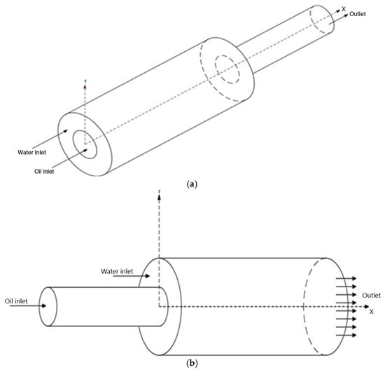
Figure 1.
(a) Core annular flow (CAF) schematic for horizontal pipe contraction. (b) Core annular flow (CAF) schematic for horizontal pipe expansion [13].
The computational domain, with an axial length of 3 m and a pipe diameter of 0.028 m, is depicted in Figure 2a. A hexahedral mesh was produced, and Figure 2b shows a third-angle projection of the mesh at the entrance and outflow. Furthermore, the mesh is grouped near the pipe wall. To verify mesh adequacy for the wall-resolved LES approach, a systematic mesh-dependence study is conducted using three mesh densities: a coarse mesh (≈238,000 cells), a medium mesh (≈472,527 cells), and a fine mesh (≈895,000 cells). The results of the medium and fine meshes showed less than a 3% variation in the predicted axial pressure gradient and oil volume fraction distribution, indicating grid independence for the studied Reynolds numbers. The final adopted mesh (472,527 cells) is, therefore, selected as an optimal compromise between accuracy and computational cost [14].
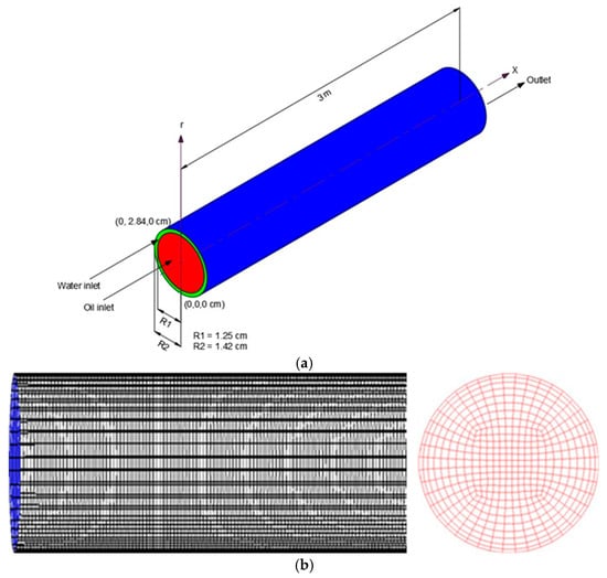
Figure 2.
(a) Dimensions and specifics of the water and oil inlet parts of the flow domain. (b) 3D unstructured grid at the inlet and outlet regions [13].
The mesh was radially clustered toward the wall using a geometric expansion ratio of less than 1.05 to ensure adequate near-wall resolution. The first cell height at the wall was approximately 0.12 mm, corresponding to y+ ≈ 0.8–1.2 for the highest simulated Reynolds number (Re = 14,728), thereby satisfying the criterion for wall-resolved LES proposed [15]. (y+ < 1). Although Figure 2b may visually appear to display coarse spacing, this effect results from visualization scaling. In the actual grid, 20–25 cells were distributed across the annular water layer at the inlet, providing sufficient resolution to accurately capture the near-wall velocity gradient and turbulent shear region.
Heavy oil flows are characterized by high Reynolds numbers and exhibit complex, fragile, and highly unpredictable behavior. The Large Eddy Simulation (LES) approach for the numerical simulation of turbulent flows in horizontal pipes is based on the concept of scale separation, which reduces computational costs. LES is primarily employed when detailed information about turbulent flow structures is required. In this method, a computational filter separates the eddies within the flow domain into large and small scales. The large-scale eddies are directly resolved using numerical calculations, while the behavior of the small-scale eddies (sub-grid scale, SGS) is modeled using an appropriate SGS model. The filtered governing equations are, thus, closed by incorporating the SGS model [16].
Efficient numerical approaches were required because wall-bounded flows simulated using LES at high Reynolds numbers involve significant computational costs. This challenge was addressed by employing a dual time-stepping technique with second-order accurate finite-difference schemes to integrate the unsteady incompressible Navier–Stokes equations [17].
2.1. LES Model
ANSYS Fluent 16.2 was used to solve the filtered Navier–Stokes equations, discretized in finite volume form. The PISO and SIMPLE algorithms were employed within the LES framework for pressure–velocity coupling. The second-order implicit time-stepping scheme in Fluent, without flux limiters, was used for temporal advancement, while linear central differencing was applied to compute the diffusion terms in the LES model. The superficial Reynolds numbers for heavy oil and water () were calculated following the approach described [18].
2.1.1. Near-Wall Treatment of the LES Model
In this study, a wall-resolved LES approach was adopted. Consequently, no wall-function or law-of-the-wall approximation was applied, and sufficiently fine grid spacing was employed to directly integrate the governing equations up to the wall. In this approach, the sub-grid scale (SGS) viscosity from the Smagorinsky model was reduced toward zero near the wall using the Van Driest wall-damping function.
Continuity equation,
Momentum equation,
= filtered (resolved) velocity component,
= filtered pressure,
= sub-grid scale (SGS) stress tensor, representing effects of unresolved small eddies.
Van Driest equation,
where A+, m, and n are. Empirical constants. In this work m = 1⁄2, n = 3, and A+ = 25 [15]. y+ is the wall normal distance. The damping only has a significant effect on y+ < 40. An important consideration for wall-resolving LES is the mesh spacing near the wall. According to the recommendation [15], for wall-resolving LES, the first mesh point away from the wall should be located at y+ < 1.
2.1.2. Initial Conditions and Boundary Conditions
The computational domain was enclosed by three boundaries: the inlet boundary, the wall boundary, and the outlet boundary. The initial conditions of the flow domain did not influence the accuracy of the results or the development of a fully established turbulent flow within the pipe. In general, the initial conditions of the computational domain affect only the computation time required to achieve a statistically steady, fully developed turbulent flow. For each given combination of heavy oil and water Reynolds numbers, the corresponding superficial velocities of water and oil are denoted as and , respectively [18].
Assuming a turbulent velocity profile, the order of magnitude of the velocity gradient at the wall can be estimated using the values of and , along with the wall no-slip boundary condition. This indicates that the large velocity gradient near the wall necessitates a small wall-normal mesh size. Fine grids are, therefore, required to adequately resolve the wall boundary layer in the wall-resolved LES approach. However, this technique demands many grid points, resulting in a significantly high computational cost. Consequently, the wall-resolved boundary condition restricts the feasibility of performing large-scale LES for many engineering applications, and the method is generally suitable only for turbulent flows at relatively low Reynolds numbers [19].
2.1.3. Boundary Condition at Pipe Inlet, Outlet, and Wall
In this model, the heavy oil fills the core of the horizontal pipe at the inlet, as shown in Figure 2a. Water fills the annular space of the horizontal pipe across the remainder of the inlet plane.
At the inlet (x = 0), separate velocity inlets are defined for the oil core and the annular water region. The water phase occupied the radial region R1 < r ≤ R2, while the oil phase occupied 0 ≤ r < R1. For each simulation case, the inlet velocities corresponded to the specified superficial velocities Usw and Uso listed in Table 1 and Table 2. The velocity profiles of both phases are prescribed as uniform (flat) distributions across their respective inlet regions, assuming fully developed turbulence would form naturally within the 3 m computational length. This approach is consistent with previous CAF simulations [1,20,21]. where uniform inlet profiles adequately reproduce the experimentally observed core annular structure. A no-slip condition is applied at the pipe wall, and a zero-gradient (Neumann) condition is imposed at the outlet. The corresponding volume fractions are initialized as αw = 1 in the annulus and αo = 1 in the core.

Table 1.
LES Simulation cases and conditions taken for simulation [13].
Table 2.
Flow conditions adopted for LES simulation.
At the outlet, the pressure outlet boundary condition in ANSYS Fluent, with zero-gauge pressure corresponding to the absolute static pressure of 101,325 Pa, is used. The diffusion fluxes for the variables in the exit direction are set at zero. A stationary no-slip boundary condition is imposed on the pipe wall, by which = 0. The y+ along the wall was estimated by the equation given in the ANSYS-Fluent users’ guide.
2.2. Simulation Setup
The simulation was set up by using the settings recommended in the Fluent User’s Guide. The problem issue was solved as a transient flow using the explicit VOF model. In this simulation, the flow is solved as turbulent when Resw > 2300. Resw is defined as the Reynolds number of water, and its numerical values are listed in the Table 1 and Table 2. The domain of this simulation is initialized with the inlet water stream limitations. ANSYS Fluent’s pressure-based segregated flow solver option is employed. The pressure integration is done using the PRESTO approach. The PISO technique provides for pressure-velocity coupling. The momentum equation is first solved using the first-order upwind technique, and then, after a few steps, the second-order upwind technique is applied. This numerical process combination produced a good convergence at a reasonable cost. The interface shape is found using the Geo-Reconstruct technique. The default values of 0.8 to 0.9 were maintained for the Under-Relaxation Factors related to density, body forces, turbulent kinetic energy, turbulent dissipation rate, and eddy viscosity. To provide a steady computation, a time step of 10−3 s is employed, resulting in a global Courant number ranging from 0.6 to 0.85. The residuals of the mesh transport equation are used to track convergence.
The convergence criteria for the simulations were set at for the absolute values of the residuals of the continuity, momentum, and turbulence equations. In addition, the water volume fraction and static pressure were monitored along several axial locations. All simulation cases were run until the observed values reached statistical stationarity.
3. Simulation Results and Validation
The simulations were conducted using the geometry shown in Figure 2a,b. The physical models of CAF, numerical simulation methodology, and the solution setup parameters have been described in the preceding section. The simulations were initially performed under the flow conditions reported [1]. to validate the numerical results. Following validation, a broader range of flow conditions was investigated using the calibrated model.
The axial pressure gradient, volume fraction discretization of the water-lubricated flow, and flow regimes were all identified by analysis of the CFD data. By contrasting the CFD results with those reported [1], the results are verified. Further investigation is done into the flow regimes, cross-sectional flow features, and related factors. We looked at the effects of the turbulence model, mesh size, initialization technique, and reconstruction strategies for the water-oil interface.
3.1. Effect on the Sub-Grid-Scale Model
The Smagorinsky–Lilly, WALE, WMLES, and WMLES S–Omega models are sub-grid-scale models available in ANSYS Fluent for two-phase flow simulations. These four models were tested to determine which one is the most appropriate for a two-phase (oil–water) flow simulation.
Figure 3 presents the predictions of the oil mass fraction obtained from various SGS models, alongside the corresponding experimental results reported [1]. All SGS models successfully reproduce the core annular flow (CAF) pattern. Among them, the WMALES S–Omega model provides the most accurate prediction of the pressure gradient. The experimental flow visualization, also taken from [1], may include some level of deformation, as the original study does not specify otherwise. In the experiments, black represents water, while white with dots indicates oil. In the LES simulations, oil is represented in red and water in blue. The figure also compares the pressure gradients predicted by the different SGS models with the experimental measurements, including the percentage differences.
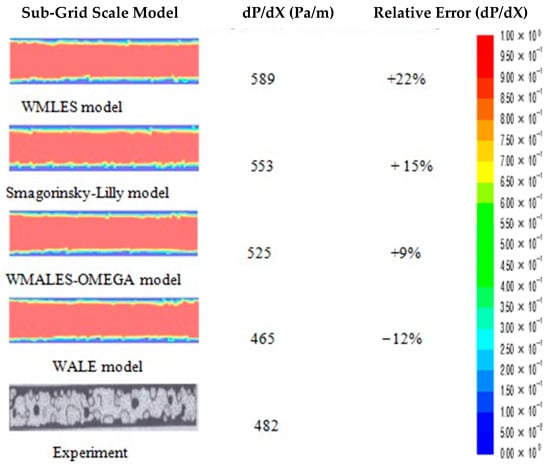
Figure 3.
Oil volume-fraction contours for LV-3 at t = 10.514 s showing results from four SGS models (Smagorinsky–Lilly, WALE, WMLES, WMLES S-Omega). Contour iso-levels and color maps are identical across panels to facilitate comparison [1].
The parameters used for the LES simulations are listed in Table 1, and the resulting turbulence variables were compared with the experimental measurements reported by [1]. The distribution of turbulence variables on the axial plane at , as predicted by the Smagorinsky–Lilly model, WALE model, WMLES model, and WMLES S–Omega model, is presented in Figure 4a–d, respectively. It was observed that the turbulence characteristics predicted by the WALE and Smagorinsky–Lilly models were comparable. Although the turbulence properties obtained using the WMLES S–Omega model are slightly lower than those predicted by the Smagorinsky–Lilly and WALE models, they remain of the same order of magnitude.
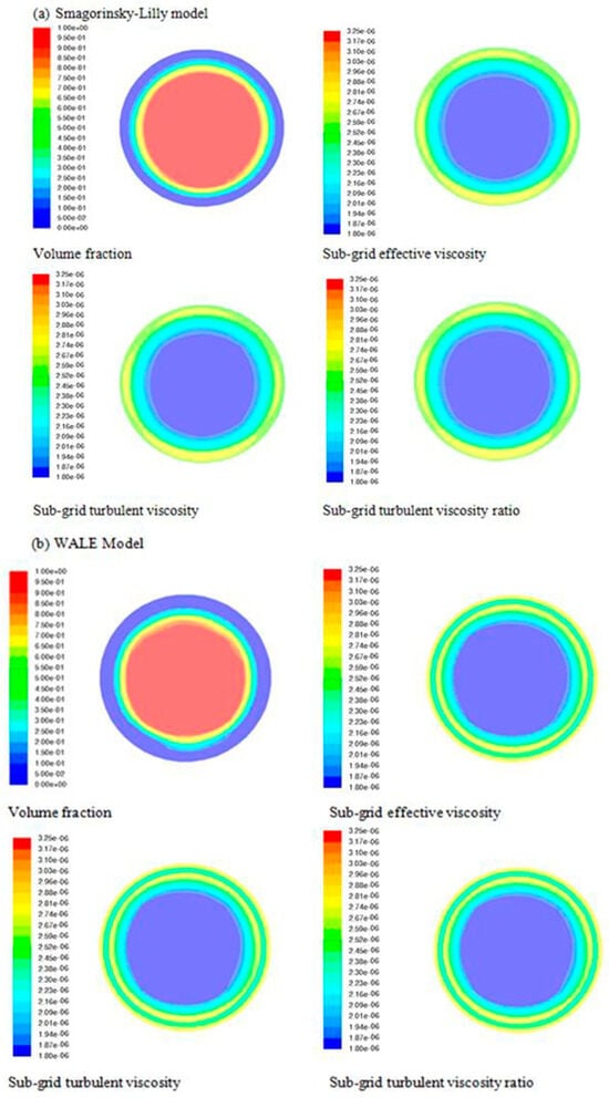
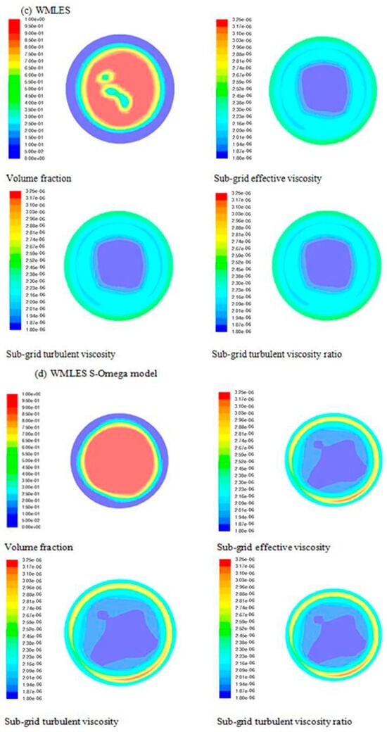
Figure 4.
(a) Distribution of the turbulence variables using the Smagorinsky–Lilly model at the same axial plane L/D = +10. (b) Distribution of the turbulence variables as determined by the WALE model at the same axial plane L/D = +10. (c) Distribution of the turbulence variables as determined by the WMLES model at the same axial plane L/D = +10. (d) Distribution of the turbulence variables as determined by the WMLES S–omega model in the same axial plane L/D = +10 [13].
3.2. Comparison of Simulation Results with Experimental Study
The flow conditions for the simulations LV-1, LV-2, and LV-3, which correspond to the experimental conditions reported by [1], are summarized in Table 2. In their experiment [1] employed water and low-viscosity oil (0.0168 Pa·s) to generate a core annular flow (CAF). Figure 5 compares the simulation results with the experimental observations, showing qualitative agreement in the flow patterns. In both the experiments and simulations, the oil–water interface in LV-1 is nearly parallel to the pipe wall and remains essentially non-wavy. For LV-3, both experimental and computational results indicate the presence of a wavy interface.
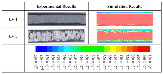
Figure 5.
Instantaneous comparison between the Smagorinsky–Lilly LES (left, t = 10.108 s) and [1] experiment (right). The image highlights an experimentally consistent wavy interface at this snapshot.
Figure 5 presents a comparison between the core annular flow (CAF) predicted by LES using the Smagorinsky–Lilly SGS model at and the experimental results reported by [1]. In the experimental visualization, black represents water, while white with inner dots represents oil. In the CFD results, color iso-levels of the oil volume fraction are used to distinguish the phases: water is shown in blue, and oil in red.
4. Results and Discussion
Cross-Sectional Flow Characteristics of CAF
The core annular flow (CAF) predicted by LES using the Smagorinsky–Lilly SGS model shows good agreement with the experimental results reported by [1]. Accordingly, this configuration was used to investigate the cross-sectional flow characteristics of CAF. For low-viscosity CAF, the axial velocity profiles and oil volume fraction distributions at different axial locations on the meridional plane are presented in Figure 6. Figure 6a illustrates a laminar flow state and a typical CAF, where the inflow volume fraction does not evolve significantly along the axial direction. The waviness of the phase interface, indicative of a turbulent flow state, is reflected in the oil volume fraction profiles shown in Figure 6b,c.
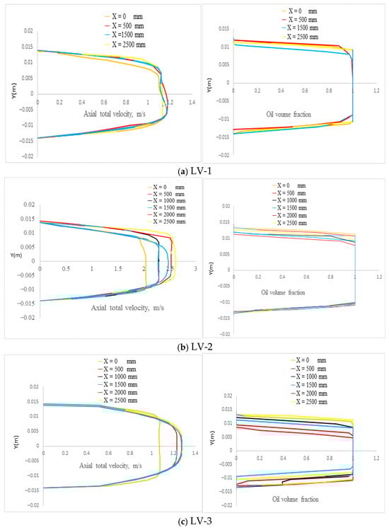
Figure 6.
Low-viscosity CAF’s oil phase volume percentage and axial velocity profiles at different axial locations. LES predictions at t = 10.2 s using the Smagorinsky–Lilly model [13].
Due to variations in the phase interface, the velocity profile along the pipe depends on the flow state and deviates from the profile expected in a single-phase flow. In particular, the velocity profile at in Figure 6a exhibits a region of reduced velocity near the upper wall. Physically, this is not expected, as the profile should be fully developed. This discrepancy is likely a numerical artifact caused by the enforced inflow boundary conditions.
The bulk velocity increases with axial distance, as shown in the velocity profiles in Figure 6b,c. This behavior resembles a pipe entry-length effect, even though the wall boundary layer has not developed sufficiently to be attributed solely to changes in the phase interface position. Overall, the flow appears to accelerate in the outlet direction, suggesting that the simulation duration may not have been sufficient to achieve a statistically stationary state.
The annular flow generates a velocity profile resembling that of a turbulent single-phase flow, as illustrated in Figure 6b,c. No significant change in the velocity gradient is observed at the water–oil interface. The simulations indicate that the maximum velocity increases from 1.15 m/s to 1.35 m/s as the water Reynolds number () rises from 6331 to 14,271.
Radial profiles of the sub-grid-scale (SGS) eddy viscosity, , on the meridional plane at various axial locations are shown in Figure 7. This figure corresponds to the CAF configuration for low-viscosity oil. The turbulence intensity is represented by the SGS eddy viscosity, , and its distribution is physically consistent, as illustrated. The results indicate that the oil core flows through the central region of the pipe, where turbulence levels are lower. At the simulated oil viscosity of 0.0168 Pa·s, the oil phase remains laminar.
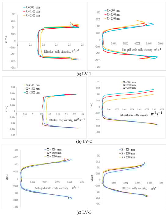
Figure 7.
Sub-grid-scale eddy viscosity μt and effective eddy viscosity of low-viscosity CAF at various axial. Predictions by LES with the SGS model by the Smagorinsky–Lilly model at time t = 10.2 s [13].
Figure 7b,c illustrates the oil–water interface region. Due to the no-slip condition at the wall and the viscosity of the oil phase, turbulence intensity is low both at the pipe wall and along the oil–water interface. In contrast, the highest sub-grid-scale (SGS) eddy viscosity is observed in the annular water layer near the pipe wall. Furthermore, an increase in the water flow rate leads to higher turbulence intensity within the annular water layer, as evidenced by the comparison between Figure 7a,b.
The LES predictions of the oil volume fraction, axial velocity profiles, and radial velocity distributions at various axial locations for heavy-oil CAF are presented in Figure 8a–c. The effects of increasing inflow momentum from HV-1 to HV-3, as well as the influence of water density from HV-1 to HV-2, are illustrated in these figures. The corresponding flow conditions are summarized in Table 3.
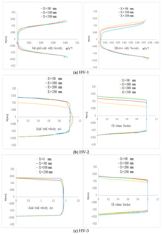
Figure 8.
Axial velocity and oil-phase volume-fraction profiles for high-viscosity core annular-flow (CAF) cases: (a) HV-1, (b) HV-2, and (c) HV-3. Results are obtained using the Smagorinsky–Lilly LES model at t = 10.2 s [13].
Table 3.
Flow conditions adopted for LES simulation (High velocity and viscosity cases) [13].
Compared to the low-velocity cases shown in Figure 6a–c, the heavy-oil CAF was investigated with an oil viscosity of 0.22 Pa·s, approximately 200 times that of water. The simulations indicate that, when the oil viscosity is much higher than that of water, the oil effectively flows within the water as a near-solid core. This behavior, supported by the present LES results, is consistent with observations reported by [20,21,22,23,24]. However, this approximation is valid only when the oil viscosity significantly exceeds that of water, as in the HV-1, HV-2, and HV-3 cases. Figure 6a–c demonstrates that when the heavy-oil viscosity is only an order of magnitude greater than the water viscosity, the oil core cannot be treated as a solid body. Comparison of Figure 8a–c shows that the velocity distribution in CAF varies with the flow state. In these figures, the developed CAF exhibits an almost symmetric velocity profile.
Figure 6a–c indicates that when the heavy-oil viscosity is only one order of magnitude greater than that of water, the oil core cannot be considered a solid body. Comparison of Figure 8a–c illustrates the influence of flow conditions on the CAF velocity distribution. In these cases, the developed CAF exhibits a nearly symmetric velocity profile.
The radial profiles of the sub-grid-scale (SGS) eddy viscosity () for the heavy-oil–water CAF at the same axial positions as in Figure 8a–c are presented in Figure 9a–c. Higher values of are observed in the annular water layer, whereas lower values are predicted within the high-viscosity oil core, reflecting the correlation between the radial distribution of SGS eddy viscosity and the oil volume fraction. Compared to the low-viscosity oil CAF (Figure 7), the SGS eddy viscosity in the oil core of the high-viscosity CAF is smaller. Specifically, in the oil core of Figure 9 ranges from approximately to , whereas in Figure 7 it is around . These results indicate that higher oil viscosity leads to reduced turbulence within the oil core.
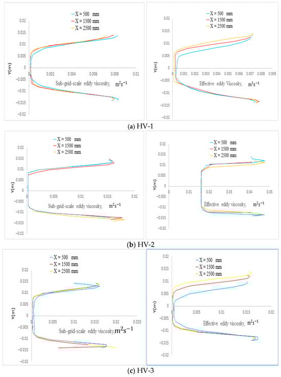
Figure 9.
Contours of time-averaged eddy-viscosity (μt) magnitude for high-viscosity CAF cases (HV-1, HV-2, HV-3) [13].
5. Conclusions
In this study, the CAF was simulated using the Volume of Fluid (VOF) model in conjunction with the Smagorinsky–Lilly sub-grid-scale model. The simulation setup and flow parameters were described in detail, and preliminary simulations were conducted to refine the configuration. Investigations were performed to assess the effects of the SGS model, mesh resolution, and initialization method for the geometric reconstruction of the water–oil interface. Spatial discretization introduced potential numerical inaccuracies, and the mesh was selected based on a mesh-dependence analysis. Both oil and water initialization methods produced results consistent with the experimental observations of [1]. To reduce computational time, the water initialization method was ultimately chosen.
The CFD results illustrate various aspects of the flow regime, pressure gradients, and cross-sectional flow characteristics. For validation purposes, the LES predictions were compared with experimental data reported by [1]. The low-viscosity oil–water flow simulations showed reasonable agreement with the experimental observations. In most simulated cases involving high-viscosity oil–water flow, no oil fouling film was observed on the pipe wall, highlighting a limitation in Fluent’s representation of wall adhesion. Differences in CAF behavior were evident in the velocity profiles for combinations of light and heavy oil with water. For light oil, the CAF velocity distribution resembles that of a turbulent single-phase flow when the water flow is turbulent. In contrast, the CAF velocity distribution with heavy oil exhibits a nearly constant velocity along the oil core. When the oil viscosity is significantly higher than that of water, the heavy oil can be assumed to flow within the annular water layer as a nearly rigid body. Furthermore, the distributions of turbulence intensity and oil volume fraction are correlated, with high turbulence intensity in the water and low turbulence intensity in the heavy oil core.
Author Contributions
Conceptualization, Methodology, Investigation and Validation, S.A.J.; Visualization and Project Administration, Y.U.A.S.; Software and Formal analysis, I.N.A.S.; Resources and Data Curation, S.S.; Conceptualization, Investigation, Writing—Original Draft Preparation, Writing—Review and Editing, D.D. All authors have read and agreed to the published version of the manuscript.
Funding
This research received no funding.
Data Availability Statement
Data may be provided by the authors on request.
Conflicts of Interest
The authors declare no conflicts of interest.
Abbreviations and Nomenclature
The following abbreviations and nomenclatures are used in this manuscript:
| CFD | Computational Fluid Dynamics |
| CAF | Core Annular Flow |
| LES | Large Eddy Simulation |
| SGS | Subgrid Scale |
| FVM | Finite Volume Method |
| R1 | Inner radius of the outer pipe |
| R2 | Outer radius of the pipe |
| Mean velocity of the mixture or bulk flow | |
| Resolved velocity component in the ith direction (filtered velocity in LES) | |
| Resolved velocity component in the jth direction (filtered velocity in LES) | |
| P | Resolved pressure (filtered pressure field) |
| Sub-grid scale (SGS) stress tensor in LES, representing the effects of unresolved eddies | |
| υ | Kinematic viscosity of the fluid m2/s |
| Spatial coordinate in the ith direction | |
| Spatial coordinate in the jth direction | |
| ⍴ | Fluid density kg/m3 |
References
- Charles, M.E.; Govier, G.W.; Hodgson, G.W. The horizontal pipeline flow of equal density of oil–water mixtures. Can. J. Chem. Eng. 1961, 39, 27–36. [Google Scholar] [CrossRef]
- Lyman, T.; Piper, E.; Riddell, A. Heavy oil mining technical and economic analysis. In Proceedings of the SPE California Regional Meeting, Long Beach, CA, USA, 11–13 April 1984. [Google Scholar]
- Martínez-Palou, R.; de Lourdes Mosqueira, M.; Zapata-Rendón, B.; Mar-Juárez, E.; Bernal-Huicochea, C.; de la Cruz Clavel-López, J.; Aburto, J. Transportation of heavy and extra-heavy crude oil by pipeline: A review. J. Pet. Sci. Eng. 2011, 75, 274–282. [Google Scholar] [CrossRef]
- Guevara, E.; Ninez, G.; Gonzalez, J. Highly viscous oil transportation methods in the Venezuelan oil industry. In Proceedings of the 15th World Petroleum Congress, Beijing, China, 12–17 October 1997. [Google Scholar]
- Kim, K.; Choi, H. Characteristics of turbulent core-annular flows in a vertical pipe. In Proceedings of the International Symposium on Turbulence Flow Phenomena, Melbourne, Australia, 30 June–3 July 2015. [Google Scholar]
- Lo, S.; Tomasello, A. Recent progress in CFD modelling of multiphase flow in horizontal and near-horizontal pipes. In Proceedings of the 7th North American Conference on Multiphase Technology, Banff, AB, Canada, 2–4 June 2010. [Google Scholar]
- Jiang, F.; Chang, J.; Huang, H.; Huang, J. A Study of the Interface Fluctuation and Energy Saving of Oil–Water Annular Flow. Energies 2022, 15, 2123. [Google Scholar] [CrossRef]
- Al Jadidi, S.; Moolya, S.; Satheesh, A. Analysis of Core Annular Flow Behavior of Water-Lubricated Heavy Crude Oil Transport. Fluids 2023, 8, 267. [Google Scholar] [CrossRef]
- Xie, B.; Jiang, F.; Lin, H.; Zhang, M.; Gui, Z.; Xiang, J. Review of Core Annular Flow. Energies 2023, 16, 1496. [Google Scholar] [CrossRef]
- Yin, X.; Li, J.; Wen, M.; Dong, X.; You, X.; Su, M.; Zeng, P.; Jing, J.; Sun, J. Study on the Hydrodynamic Performance and Stability Characteristics of Oil–Water Annular Flow through a 90° Elbow Pipe. Sustainability 2023, 15, 6785. [Google Scholar] [CrossRef]
- Lv, G.; He, L. Oil–Water Two-Phase Flow with Three Different Crude Oils: Flow Structure, Droplet Size and Viscosity. Energies 2024, 17, 1573. [Google Scholar] [CrossRef]
- Kim, K.; Choi, H. Characteristics of Turbulent Core–Annular Flow with Water-Lubricated High Viscosity Oil in a Horizontal Pipe. J. Fluid Mech. 2024, 986, A19. [Google Scholar] [CrossRef]
- Jadidi, A.; Saleh, S.J. Lubricated Transport of Heavy Oil Investigated by CFD. Ph.D. Thesis, University of Leicester, Leicester, UK, 2017. Available online: https://hdl.handle.net/2381/40986 (accessed on 19 December 2017).
- Versteeg, H.K.; Malalasekera, W. An Introduction to Computational Fluid Dynamics: The Finite Volume Method; Pearson Education Ltd.: Harlow, UK, 2007. [Google Scholar]
- Piomelli, U. Large-eddy simulations: Where we stand. In Advances in DNS/LES; Liu, C., Liu, Z., Eds.; AFOSR: New Orleans, LA, USA, 1997; pp. 93–104. [Google Scholar]
- Sagaut, P. Large Eddy Simulation for Incompressible Flows: An Introduction; Springer: Berlin/Heidelberg, Germany, 2006. [Google Scholar]
- Ferziger, J.H.; Perić, M. Computational Methods for Fluid Dynamics; Springer: Berlin/Heidelberg, Germany, 2002. [Google Scholar]
- Balakhrisna, T.; Ghosh, S.; Das, G.; Das, P.K. Oil-water flow through sudden contraction and expansion in a horizontal pipe-phase distribution and pressure drop. Int. J. Multiph. Flow 2010, 1, 13–24. [Google Scholar] [CrossRef]
- Moin, P.; Kim, J. Numerical Investigation of Turbulent Channel Flow. J. Fluid Mech. 1982, 118, 341–377. [Google Scholar] [CrossRef]
- Ooms, G.; Vuik, C.; Poesio, P. Core annular flow through a horizontal pipe: Hydrodynamic counter balancing of buoyancy force on core. Phys. Fluids 2007, 19, 92–103. [Google Scholar] [CrossRef]
- Ooms, G.; Poesio, P. Stationary core annular flow through a horizontal pipe. J. Phys. Rev. E 2003, 68, 663–701. [Google Scholar] [CrossRef] [PubMed]
- Ooms, G.; Pourquie, M.J.B.M.; Poesio, P. Numerical study of eccentric core annular flow. Int. J. Multiph. Flow 2012, 42, 74–79. [Google Scholar] [CrossRef]
- Zhang, H.-Q.; Sridhar, S.; Sarica, C.; Pereyra, E.J. Experiments and model assessment on high-viscosity oil/water inclined pipe flows. In Proceedings of the SPE Annual Technical Conference and Exhibition, Denver, CO, USA, 30 October–2 November 2011. [Google Scholar]
- Zhang, H.-Q.; Vuong, D.H.; Sarica, C. Modeling high-viscosity oil/water concurrent flow in horizontal and vertical pipes. SPE J. 2012, 17, 243–250. [Google Scholar] [CrossRef]
Disclaimer/Publisher’s Note: The statements, opinions and data contained in all publications are solely those of the individual author(s) and contributor(s) and not of MDPI and/or the editor(s). MDPI and/or the editor(s) disclaim responsibility for any injury to people or property resulting from any ideas, methods, instructions or products referred to in the content. |
© 2025 by the authors. Licensee MDPI, Basel, Switzerland. This article is an open access article distributed under the terms and conditions of the Creative Commons Attribution (CC BY) license (https://creativecommons.org/licenses/by/4.0/).