Solution of the Vector Three-Dimensional Inverse Problem on an Inhomogeneous Dielectric Hemisphere Using a Two-Step Method

Abstract

This work is devoted to the development and implementation of a two-step method for solving the vector three-dimensional inverse diffraction problem on an inhomogeneous dielectric scatterer having the form of a hemisphere characterized by piecewise constant permittivity. The original boundary value problem for Maxwell’s equations is reduced to a system of integro-differential equations. An integral formulation of the vector inverse diffraction problem is proposed and the uniqueness of the solution of the first-kind integro-differential equation in special function classes is established. A two-step method for solving the vector inverse diffraction problem on the hemisphere is developed. Unlike traditional approaches, the two-step method for solving the inverse problem is non-iterative and does not require knowledge of the exact initial approximation. Consequently, there are no issues related to the convergence of the numerical method. The results of calculations of approximate solutions to the inverse problem are presented. It is shown that the two-step method is an efficient approach to solving vector problems in near-field tomography.

1. Introduction

Inverse vector diffraction problems of electromagnetic waves in three-dimensional space are of great interest in medical diagnostics, non-destructive testing, and defectoscopy [1,2,3]. One of the most common approaches to solving these problems involves minimizing certain error functionals using Tikhonov regularization and iterative methods that require the selection of a good initial approximation [4,5,6,7].

This paper discusses a non-iterative approach to solving the three-dimensional vector inverse problem of reconstructing the inhomogeneity of a dielectric body in the form of a hemisphere based on near-field electromagnetic measurements. It is necessary to find the unknown piecewise continuous permittivity (or corresponding refractive index) of a bounded scatterer in ${\mathbb{R}}^3$, a hemisphere.

Unlike traditional approaches, the two-step method for solving the inverse problem is non-iterative, and therefore, does not require selecting a good initial approximation. This advantage of the two-step method is crucial because the selection of a good initial approximation in iterative methods is a separate and challenging task. Additionally, there are no issues related to the convergence of the numerical method. In many approaches to solving inverse problems, the convergence of iterative methods is not rigorously proven and estimates of convergence rates are not obtained. In contrast, the two-step non-iterative method that we develop allows us to directly solve the system of linear algebraic equations that arises when solving the inverse problem using well-known methods. The main drawback of our method is poor conditioning of the matrix of the linear algebraic equation system. However, this is not a drawback of the method itself; in fact, it is a property of inverse problems in general. On the other hand, the solution techniques of such systems of linear algebraic equations are well developed at present. In our case, standard regularization methods and the construction of preconditioners have proven to be efficient.

The paper describes, justifies, and applies a two-step method that has been successfully used previously to solve other scalar and vector inverse scattering problems [8,9,10,11,12].

The article consists of four sections.

In the first section, the direct problem of diffraction of a monochromatic electromagnetic wave by a bounded scatterer with a given constant permeability of vacuum and variable permittivity $\epsilon \left(x\right)$ of the scatterer is formulated. The initial boundary problem for Maxwell’s equations is reduced to a system consisting of a singular integro-differential equation for the electric field in the inhomogeneity domain and an integral representation of the total electric field outside the scatterer. The main results concerning the solvability of the direct diffraction problem are presented.

The second section is devoted to the theoretical study of the inverse diffraction problem, which involves finding the function of the unknown permittivity of a hemispherical body. The hemisphere shape is chosen with the aim of applying the solution results to breast cancer diagnosis. We consider complete integral formulation of the inverse problem. The first step of the proposed method consists in solving a linear integro-differential equation of the first kind with respect to the polarization current. In the second step, the permittivity is explicitly expressed in terms of known functions.

The third section demonstrates that the integro-differential equation of the first kind has not more than one solution in finite-dimensional spaces of piecewise constant functions.

The fourth section describes the results of numerical tests.

The main application area of the results of this article is the early diagnosis of breast cancer using microwave tomography.

2. Direct Problem: Formulation and Main Results

Let $Q\subset {\mathbb{R}}^3$ be a hemisphere, then its boundary $\partial Q$ is a piecewise-smooth surface consisting of two surfaces of class $C^{\infty }$.

We assume that the dielectric body Q is isotropic and inhomogeneous and that the hemisphere is characterized by constant permeability ${\mu }_0>0$ and permittivity function $\epsilon \left(x\right)\in C^{\infty }\left(\overline{Q}\right)$.

Introduce the relative permittivity ${\epsilon }_r=\epsilon /{\epsilon }_0$ and suppose that at each point $x\in \overline{Q}$ there exists a complex-valued function

$${({\epsilon }_r\left(x\right)-1)}^{-1}.$$

(1)

The free space ${\mathbf{R}}^3\setminus \overline{Q}$ is assumed to be homogeneous with constant values: ${\epsilon }_0>0$, ${\mu }_0>0$ (vacuum).

The field is excited by a point source at $x_0\in {\mathbf{R}}^3\setminus \overline{Q}$, generating an electromagnetic wave ${\mathbf{E}}_0,{\mathbf{H}}_0\in C^{\infty }({\mathbf{R}}^3\setminus x_0)$, satisfying Maxwell’s equations in ${\mathbf{R}}^3\setminus x_0$:

$$\mathrm{rot}{\mathbf{H}}_0=-i\omega {\epsilon }_0{\mathbf{E}}_0,\mathrm{rot}{\mathbf{E}}_0=i\omega {\mu }_0{\mathbf{H}}_0.$$

(2)

The total field is represented as the sum of the incident and scattered fields:

$$\mathbf{E}={\mathbf{E}}_0+{\mathbf{E}}_s,\mathbf{H}={\mathbf{H}}_0+{\mathbf{H}}_s.$$

(3)

The solution to the direct diffraction problem is the total electromagnetic field $\mathbf{E},\mathbf{H}$ belonging to function classes

$$\mathbf{E},\mathbf{H}\in C^2({\mathbb{R}}^3\setminus \partial Q)\cap C\left(\overline{Q}\right)\cap C({\mathbb{R}}^3\setminus Q),$$

(4)

satisfying in ${\mathbb{R}}^3\setminus \partial Q$ Maxwell’s equations,

$$\mathrm{rot}\mathbf{H}=-i\omega \epsilon \mathbf{E},\mathrm{rot}\mathbf{E}=i\omega {\mu }_0\mathbf{H},$$

(5)

the conditions of continuity for the tangential components at the boundary of the inhomogeneity domain,

$$\left[{\mathbf{E}}_{\tau }\right]{{|}_{\partial Q}=\left[{\mathbf{H}}_{\tau }\right]|}_{\partial Q}=0,$$

(6)

the conditions of finiteness of energy in any bounded volume of space,

$$\mathbf{E},\mathbf{H}\in L_{2,\mathrm{loc}}\left({\mathbf{R}}^3\right),$$

(7)

and the Silver–Müller radiation conditions at infinity for the scattered field [13],

$$\begin{array}{cc}{\mathbf{H}}_s\times {\mathbf{e}}_r-{\mathbf{E}}_s=o\left(r^{-1}\right),& {\mathbf{E}}_s\times {\mathbf{e}}_r+{\mathbf{H}}_s=o\left(r^{-1}\right),\\ {\mathbf{E}}_s,{\mathbf{H}}_s=O\left(r^{-1}\right),& r\to \infty ,\end{array}$$

(8)

where $k_0^2={\omega }^2{\epsilon }_0{\mu }_0$ is the wavenumber and ${\mathbf{e}}_r=\mathbf{x}/r$, $r=\left|\mathbf{x}\right|$, $\mathbf{x}={(x_1,x_2,x_3)}^T$; the limiting relations in (8) are uniformly satisfied in all directions.

Definition 1. 

A solution $\mathbf{E},\mathbf{H}$ to problem (2)–(8), satisfying conditions (4), is called quasiclassical.

We formulate the main results on the solvability of the direct diffraction problem.

Proposition 1. 

Suppose the permittivity satisfies in $\overline{Q}$ the conditions

$${\epsilon }_r\in C^{\infty }\left(\overline{Q}\right),\mathrm{Re}{\epsilon }_r>1,\mathrm{Im}{\epsilon }_r\ge 0,$$

(9)

and outside $\overline{Q}$, $\epsilon ={\epsilon }_0$ and $\mu ={\mu }_0$. Then, the diffraction problem (2)–(8) has at most one quasiclassical solution.

The boundary value problem (2)–(8) can be reduced to a system consisting of an integro-differential equation in the inhomogeneity domain,

$$\mathbf{E}\left(x\right)-(k_0^2+\mathrm{grad}\mathrm{div})\underset{Q}{\int }G(x,y)({\epsilon }_r\left(y\right)-1)\mathbf{E}\left(y\right)dy={\mathbf{E}}_0\left(x\right),x\in Q,$$

(10)

and an integral representation of the field outside the body,

$$\mathbf{E}\left(x\right)={\mathbf{E}}_0\left(x\right)+(k_0^2+\mathrm{grad}\mathrm{div})\underset{Q}{\int }G(x,y)({\epsilon }_r\left(y\right)-1)\mathbf{E}\left(y\right)dy,x\in {\mathbf{R}}^3\setminus \overline{Q}$$

(11)

where $G(x,y)={\displaystyle \frac{e^{i{k}_0|x-y|}}{4\pi |x-y|}}$.

The magnetic field everywhere is expressed through the electric field by the formula

$$\mathbf{H}={\displaystyle \frac{1}{i\omega {\mu }_0}}\mathrm{rot}\mathbf{E}.$$

(12)

The following proposition states the equivalence of the boundary problem and the integro-differential equation.

Proposition 2. 

If the boundary value problem (2)–(8) has a quasiclassical solution $\mathbf{E},\mathbf{H},$ then the vector function $\mathbf{E}\in C\left(\overline{Q}\right)\cap {\mathbf{L}}_2\left(Q\right)$ satisfies the integro-differential Equation (11). Conversely, if $\mathbf{E}\in {\mathbf{L}}_2\left(Q\right)$ satisfies Equation (11), then the boundary value problem (2)–(8) has a quasiclassical solution $\mathbf{E},\mathbf{H},$ expressed by Formulas (10)–(12).

Proposition 3. 

Suppose the permittivity satisfies conditions $\epsilon \in C^{\infty }\left(\overline{Q}\right)$ and $\mathrm{Re}{\epsilon }_r>1$, $\mathrm{Im}{\epsilon }_r\ge 0$ at $x\in \overline{Q}$. Then, the operator

$$A\mathbf{E}\left(x\right):=\mathbf{E}\left(x\right)-(k_0^2+\mathrm{grad}\mathrm{div})\underset{Q}{\int }G(x,y)({\epsilon }_r\left(y\right)-1)\mathbf{E}\left(y\right)dy$$

is continuously invertible in ${\mathbf{L}}_2\left(Q\right)$.

Proofs of Propositions 1–3 can be found in Refs. [14,15].

3. Inverse Problem Formulation

In a homogeneous three-dimensional space ${\mathbf{R}}^3$ characterized by a wavenumber $k_0>0$, consider, in the spherical coordinates $x=\{r,\phi ,\theta \},r\ge 0,0\le \phi \le 2\pi ,0\le \theta \le \pi$, the vector inverse problem of reconstructing the inhomogeneity of an isotropic dielectric hemisphere Q (without boundary):

$$Q=\{x:0\le r\le R,0\le \phi \le 2\pi ,0\le \theta \le {\displaystyle \frac{\pi }{2}}\}.$$

(13)

Introduce a uniform grid on Q with the nodes

$$r_{i_1}={\displaystyle \frac{R}{n_1}}{i}_1,0\le i_1\le n_1,{\phi }_{i_2}={\displaystyle \frac{2\pi }{n_2}}{i}_2,0\le i_2\le n_2,{\theta }_{i_3}={\displaystyle \frac{\pi /2}{n_3}}{i}_3,0\le i_3\le n_3.$$

Divide Q into elementary cells:

$$Q_{i_1{i}_2{i}_3}=\{x:r_{i_1}<r<r_{i_1+1},{\phi }_{i_2}<\phi <{\phi }_{i_2+1},{\theta }_{i_3}<\theta <{\theta }_{i_3+1}\},0\le i_k\le n_k-1.$$

(14)

Introduce piecewise constant functions ${\chi }_{i_1{i}_2{i}_3}$:

$${\chi }_{i_1{i}_2{i}_3}\left(x\right)=\left\{\begin{array}{cc}1,\hfill & \mathrm{if}x\in Q_{i_1{i}_2{i}_3},\hfill \\ 0,\hfill & \mathrm{if}x\notin Q_{i_1{i}_2{i}_3}.\hfill \end{array}\right.$$

(15)

Assume that the domain Q is characterized by permeability ${\mu }_0>0$ and the piecewise constant permittivity function $\epsilon \left(x\right)={\epsilon }_r\left(x\right){\epsilon }_0.$ Specifically,

$$\epsilon \left(x\right)={\epsilon }_{i_1{i}_2{i}_3},x\in Q_{i_1{i}_2{i}_3}.$$

(16)

The permittivity at the boundaries $\partial Q_{i_1{i}_2{i}_3}$ can be defined as the limit of $\epsilon \left(x\right)$ in one of the adjacent cells.

Introducing a multi-index $\mathbf{i}=\left(i_1{i}_2{i}_3\right),$ represent the function $\epsilon \left(x\right)$ at each $x\in Q$ by the equation

$$\epsilon \left(x\right)=\sum _{\mathbf{i}}{\epsilon }_{\mathbf{i}}\left(x\right){\chi }_{\mathbf{i}}\left(x\right).$$

(17)

Consider a certain bounded domain D such that $\overline{D}\cap \overline{Q}=\varnothing .$ Assume that for points $x\in D$ the values of the total field at a fixed frequency $\omega >0$ are known.

When setting up the inverse diffraction problem, use the system of integral Equations (10) and (11), defining the dependence of the field $\mathbf{E}\left(x\right)$ on the permittivity $\epsilon \left(x\right)$ and the incident wave ${\mathbf{E}}_0\left(x\right).$

Formulation of the inverse diffraction problem. It is required to reconstruct the function $\epsilon \left(x\right)$ in the inhomogeneity domain Q from the measurements of the total field $\mathbf{E}\left(x\right)$ at points in the domain D using the equation

$$(k_0^2+\mathrm{grad}\mathrm{div})\underset{Q}{\int }G(x,y)({\epsilon }_r\left(y\right)-1)\mathbf{E}\left(y\right)dy=\mathbf{E}\left(x\right)-{\mathbf{E}}_0\left(x\right),x\in D,$$

(18)

taking into account the equation in the inhomogeneity domain Q,

$$\mathbf{E}\left(x\right)-(k_0^2+\mathrm{grad}\mathrm{div})\underset{Q}{\int }G(x,y)({\epsilon }_r\left(y\right)-1)\mathbf{E}\left(y\right)dy={\mathbf{E}}_0\left(x\right),x\in Q.$$

(19)

Description of the Two-Step Method for Solving the Inverse Diffraction Problem. Introduce in the domain Q the vector function

$$\mathbf{J}\left(x\right):=({\epsilon }_r\left(x\right)-1)\mathbf{E}\left(x\right),$$

assuming that everywhere in Q the condition $|{\epsilon }_r\left(x\right)|\ge \tilde{\epsilon }>1$ is fulfilled. Then, from the representation of the field outside the scatterer, derive the equation for $\mathbf{J}\left(x\right)$,

$$(k_0^2+\mathrm{grad}\mathrm{div})\underset{Q}{\int }G(x,y)\mathbf{J}\left(y\right)dy=\mathbf{E}\left(x\right)-{\mathbf{E}}_0\left(x\right),x\in D,$$

(20)

and rewrite the equation in the inhomogeneity domain in the form

$${\displaystyle \frac{\mathbf{J}\left(x\right)}{{\epsilon }_r\left(x\right)-1}}-(k_0^2+\mathrm{grad}\mathrm{div})\underset{Q}{\int }G(x,y)\mathbf{J}\left(y\right)dy={\mathbf{E}}_0\left(x\right),x\in Q.$$

(21)

The two-step method for recovering the permittivity in Q consists in the following. The first step is as follows: from the known values of the incident field ${\mathbf{E}}_0\left(x\right)$ and the total field $\mathbf{E}\left(x\right)$ in the domain D, find the current $\mathbf{J}\left(x\right)$ in Q from Equation (20). The second step: calculate ${\epsilon }_r\left(x\right)$ in Q explicitly using Equation (21).

4. Uniqueness of the Solution to the Integro-Differential Equation

To approximate the calculation of $\mathbf{J}$, the collocation method with finite basis functions is employed. Initially, suppose that $\mathbf{J}$ is represented as a piecewise constant function:

$$\mathbf{J}\left(x\right)=\sum _{\mathbf{i}}{\mathbf{J}}_{\mathbf{i}}{\chi }_{\mathbf{i}}\left(x\right),$$

(22)

where ${\mathbf{J}}_{\mathbf{i}}\in {\mathbb{C}}^3$ are unknown (vector) coefficients, and ${\chi }_{\mathbf{i}}\left(x\right)$ are characteristic functions of the sets $Q_{\mathbf{i}}$ (on the faces of $Q_{\mathbf{i}}$ the current may be defined by any of the constant values).

The uniqueness of the solution to Equation (20) can be verified in the class of piecewise constant functions $\mathbf{J}\left(x\right)$.

Theorem 1. 

Let the body Q be partitioned into $n_1{n}_2{n}_3$ cells $Q_{\mathbf{i}}$. Taking into account Equations (20) and (21),

$$(k_0^2+\mathrm{grad}\mathrm{div})\underset{Q}{\int }G(x,y)\mathbf{J}\left(y\right)dy={\mathbf{E}}_s\left(x\right),x\in D,\overline{D}\cap \overline{Q}=\varnothing ,{\mathbf{E}}_s\in C^{\infty }\left(\overline{D}\right),$$

(23)

the following holds: the problem has not more than one piecewise constant solution $\mathbf{J}\left(x\right)$ for all $k_0>0$ except, possibly, a finite number of $k_0$ values.

The proof is analogous to that presented in [11] for the case of a parallelepiped instead of a hemisphere.

From Theorem 1, it follows that the solution to the inverse diffraction problem for the case of piecewise constant currents J is unique due to the uniqueness of the representation of $\epsilon \left(x\right)$ according to Equation (21).

Remark 1 

(on the existence of solutions). Suppose that the right-hand side of Equation (20) belongs to the linear span of the functions

$$(k_0^2+\mathrm{grad}\mathrm{div})\underset{Q}{\int }G(x,y)\mathbf{J}\left(y\right)dy$$

on a given fixed grid in Q. Then, the operator of Equation (20) can be considered as a mapping acting in finite-dimensional spaces. This mapping will be invertible due to Theorem 1.

5. Numerical Method for Solving the Direct and Inverse Problems

Both the direct and inverse problems are solved using the collocation method. To implement this method, it is necessary to choose basis functions and collocation nodes.

The simplest choice of basis functions is piecewise constant functions, as described in (15), where the support is one elementary cell. This type of basis function has been considered in [8,9,10,11,12]. A disadvantage of this choice is that it is not possible to include the divergence operation under the integral sign and “transfer” the operation to the basis function, thus necessitating the solution of a singular integro-differential equation. This requires the use of special methods to account for the singularities in integrals.

In this work, another option for choosing basis functions is proposed and is described below. In this case, we only need to calculate integrals with weak singularities.

We introduce three types of basis functions, the supports of which are two adjacent cells. Along one coordinate, these functions are piecewise linear, and along the other two, they are piecewise constant.

We define grid steps for variables as $h_1=R/n_1$, $h_2=2\pi /n_2$, $h_3=\pi /\left(2n_3\right)$. The basis functions are defined as

$$v_{i_1{i}_2{i}_3}^{\left(r\right)}\left(x\right)=\left\{\begin{array}{cc}1-\left|r-r_{i_1}\right|/h_1,\hfill & x\in Q_{i_1-1,i_2{i}_3}\cup Q_{i_1{i}_2{i}_3},\hfill \\ 0,\hfill & x\notin Q_{i_1-1,i_2{i}_3}\cup Q_{i_1{i}_2{i}_3}\hfill \end{array}\right.$$

(24)

$$v_{i_1{i}_2{i}_3}^{\left(\phi \right)}\left(x\right)=\left\{\begin{array}{cc}1-\left|\phi -{\phi }_{i_2}\right|/h_2,\hfill & x\in Q_{i_1{i}_2-1,i_3}\cup Q_{i_1{i}_2{i}_3},\hfill \\ 0,\hfill & x\notin Q_{i_1{i}_2-1,i_3}\cup Q_{i_1{i}_2{i}_3}\hfill \end{array}\right.$$

(25)

$$v_{i_1{i}_2{i}_3}^{\left(\theta \right)}\left(x\right)=\left\{\begin{array}{cc}1-\left|\theta -{\theta }_{i_3}\right|/h_3,\hfill & x\in Q_{i_1{i}_2{i}_3-1}\cup Q_{i_1{i}_2{i}_3},\hfill \\ 0,\hfill & x\notin Q_{i_1{i}_2{i}_3-1}\cup Q_{i_1{i}_2{i}_3}\hfill \end{array}\right.$$

(26)

In implementing the collocation method, it is necessary to compute integrals of the form

$$(k_0^2+\mathrm{grad}\mathrm{div})\underset{Q}{\int }G(x,y){\mathbf{J}}_N\left(y\right)dy,$$

where ${\mathbf{J}}_N$ is the approximate solution.

The operations of divergence and gradient in spherical coordinates for an arbitrary scalar function $\Phi$ and vector function $\mathbf{F}$ at the point $x=(r,\phi ,\theta )$ are

$$\mathrm{grad}\Phi ={\displaystyle \frac{\partial \Phi }{\partial r}}\mathbf{r}+{\displaystyle \frac{1}{rsin\theta }}{\displaystyle \frac{\partial \Phi }{\partial \phi }}\mathit{\phi }+{\displaystyle \frac{1}{r}}{\displaystyle \frac{\partial \Phi }{\partial \theta }}\mathit{\theta },$$

(27)

$$\mathrm{div}\mathbf{F}={\displaystyle \frac{1}{r^2}}{\displaystyle \frac{\partial \left(r^2{\mathbf{F}}_r\right)}{\partial r}}+{\displaystyle \frac{1}{rsin\theta }}{\displaystyle \frac{\partial {\mathbf{F}}_{\phi }}{\partial \phi }}+{\displaystyle \frac{1}{rsin\theta }}{\displaystyle \frac{\partial ({\mathbf{F}}_{\theta }sin\theta )}{\partial \theta }},$$

(28)

where $\mathbf{r},\mathit{\phi },\mathit{\theta }$ are unit vectors in the corresponding directions. The vector basis functions are formed as follows:

$${\mathbf{v}}_{i_1{i}_2{i}_3}^{\left(r\right)}\left(x\right)=v_{i_1{i}_2{i}_3}^{\left(r\right)}\left(x\right)\mathbf{r}\left(x\right),{\mathbf{v}}_{i_1{i}_2{i}_3}^{\left(\phi \right)}\left(x\right)=v_{i_1{i}_2{i}_3}^{\left(\phi \right)}\left(x\right)\mathit{\phi }\left(x\right),{\mathbf{v}}_{i_1{i}_2{i}_3}^{\left(\theta \right)}\left(x\right)=v_{i_1{i}_2{i}_3}^{\left(\theta \right)}\left(x\right)\mathit{\theta }\left(x\right).$$

(29)

Thus, within their supports, we compute the divergence of the basis functions (29) using Formulas (24)–(26) and (28):

$$\mathrm{div}{\mathbf{v}}_{i_1{i}_2{i}_3}^{\left(r\right)}\left(x\right)={\displaystyle \frac{2}{r}}{v}_{i_1{i}_2{i}_3}^{\left(r\right)}\left(x\right)-\mathrm{sign}(r-r_{i_1})/h_1,$$

(30)

$$\mathrm{div}{\mathbf{v}}_{i_1{i}_2{i}_3}^{\left(\phi \right)}\left(x\right)=-{\displaystyle \frac{1}{rsin\theta }}\mathrm{sign}(\phi -{\phi }_{i_2})/h_2,$$

(31)

$$\mathrm{div}{\mathbf{v}}_{i_1{i}_2{i}_3}^{\left(\theta \right)}\left(x\right)={\displaystyle \frac{cot\theta }{r}}{v}_{i_1{i}_2{i}_3}^{\left(\theta \right)}\left(x\right)-{\displaystyle \frac{1}{r}}\mathrm{sign}(\theta -{\theta }_{i_3})/h_3.$$

(32)

Due to the choice of basis functions, the divergence is computed in the usual manner (not as for a generalized function) and is a piecewise continuous function. Outside the supports of the basis functions, their divergence is zero.

Further, each component of the current (approximate solution) is sought as a linear combination of the corresponding basis functions with unknown coefficients:

$${\mathbf{J}}_N^{\left(r\right)}\left(x\right)=\sum _{\mathbf{i}}{J}_{\mathbf{i}}^{\left(r\right)}{\mathbf{v}}_{\mathbf{i}}^{\left(r\right)}\left(x\right),$$

(33)

$${\mathbf{J}}_N^{\left(\phi \right)}\left(x\right)=\sum _{\mathbf{i}}{J}_{\mathbf{i}}^{\left(\phi \right)}{\mathbf{v}}_{\mathbf{i}}^{\left(\phi \right)}\left(x\right),$$

(34)

$${\mathbf{J}}_N^{\left(\theta \right)}\left(x\right)=\sum _{\mathbf{i}}{J}_{\mathbf{i}}^{\left(\theta \right)}{\mathbf{v}}_{\mathbf{i}}^{\left(\theta \right)}\left(x\right).$$

(35)

Then, for the approximate solution, we have ${\mathbf{J}}_N\left(x\right)={\mathbf{J}}_N^{\left(r\right)}\left(x\right)+{\mathbf{J}}_N^{\left(\phi \right)}\left(x\right)+{\mathbf{J}}_N^{\left(\theta \right)}\left(x\right)$. It is important to note that the normal component of the approximate solution is zero at the smooth points of the boundary $\partial Q$, ${\mathbf{J}}_N\left(x\right)·\nu \left(x\right)=0$ (here $\nu \left(x\right)$ is the external normal to the boundary at the point $x\in \partial Q$). Moreover, it is evident that the introduced basis functions possess the property of approximation in the $L_2\left(Q\right)$ space.

Remark 2. 

Since the solutions at $\phi =0$ and $\phi =2\pi$ coincide, it is necessary to add basis functions with index $i_2=n_2$, i.e., $0\le i_1\le n_1-1$, $0\le i_2\le n_2$, $0\le i_3\le n_3-1$.

For the numerical implementation, it is necessary to compute the divergence of the volume integral.

Lemma 1. 

The following relation is valid for any $x\in {\mathbf{R}}^3$:

$${\mathrm{div}}_x\underset{Q}{\int }G(x,y){\mathbf{J}}_N\left(y\right)dy=\underset{Q}{\int }G(x,y)\mathrm{div}{\mathbf{J}}_N\left(y\right)dy.$$

(36)

Proof. 

Indeed,

$${\mathrm{div}}_x\underset{Q}{\int }G(x,y){\mathbf{J}}_N\left(y\right)dy=\underset{Q}{\int }{\mathrm{grad}}_{x}G(x,y)·{\mathbf{J}}_N\left(y\right)dy=-\underset{Q}{\int }{\mathrm{grad}}_{y}G(x,y)·{\mathbf{J}}_N\left(y\right)dy.$$

Further,

$$-{\int }_Q{\mathrm{grad}}_{y}G(x,y)·{\mathbf{J}}_N\left(y\right)dy=-\underset{Q}{\int }{\mathrm{div}}_y\left(G(x,y){\mathbf{J}}_N\left(y\right)\right)dy+\underset{Q}{\int }G(x,y)\mathrm{div}{\mathbf{J}}_N\left(y\right)dy.$$

By the Gauss–Ostrogradsky theorem, due to the zero normal component ${\mathbf{J}}_N\left(x\right)$ on $\partial Q$, we have

$$\underset{Q}{\int }{\mathrm{div}}_y\left(G(x,y){\mathbf{J}}_N\left(y\right)\right)dy=0,$$

which proves the lemma. □

Note that for $x\in \overline{Q}$, the improper integrals have a weak singularity and converge absolutely.

Formula (36) can be obtained in Cartesian coordinates and applied in spherical coordinates using the invariance of the gradient and divergence operations relative to the coordinate system.

Now, compute

$${\mathrm{grad}}_x{\mathrm{div}}_x\underset{Q}{\int }G(x,y){\mathbf{J}}_N\left(y\right)dy=\underset{Q}{\int }{\mathrm{grad}}_{x}G(x,y)\mathrm{div}{\mathbf{J}}_N\left(y\right)dy$$

(37)

as an improper absolutely converging integral because the singularity of the kernel is of an order $O\left(\right|x-y{|}^{-2})$ when $|x-y|\to 0$ (weak singularity). Formulas (30)–(32) are used to compute $\mathrm{div}{\mathbf{J}}_N\left(y\right)$.

We have

$$|x-y|=\sqrt{r^2+r_0^2-2r{r}_0(cos(\phi -{\phi }_0)sin\theta sin{\theta }_0+cos\theta cos{\theta }_0)},$$

(38)

where $x=(r,\phi ,\theta )$ and $y=(r_0,{\phi }_0,{\theta }_0)$. Introduce the function $G1\left(t\right):=\left(i{k}_0-{\displaystyle \frac{1}{t}}\right){\displaystyle \frac{e^{i{k}_{0}t}}{4\pi t}}$. Then, by Formula (27), we find

$${\mathrm{grad}}_{x}G(x,y)=G1\left(\right|x-y\left|\right)\left({\displaystyle \frac{\partial |x-y|}{\partial r}}\mathbf{r}+{\displaystyle \frac{1}{rsin\theta }}{\displaystyle \frac{\partial |x-y|}{\partial \phi }}\mathit{\phi }+{\displaystyle \frac{1}{r}}{\displaystyle \frac{\partial |x-y|}{\partial \theta }}\mathit{\theta }\right),$$

(39)

where

$${\displaystyle \frac{\partial |x-y|}{\partial r}}={\displaystyle \frac{r-r_0(cos(\phi -{\phi }_0)sin\theta sin{\theta }_0+cos\theta cos{\theta }_0)}{|x-y|}},$$

(40)

$${\displaystyle \frac{\partial |x-y|}{\partial \phi }}={\displaystyle \frac{r{r}_{0}sin(\phi -{\phi }_0)sin\theta sin{\theta }_0}{|x-y|}},$$

(41)

$${\displaystyle \frac{\partial |x-y|}{\partial \theta }}={\displaystyle \frac{-r{r}_0(cos(\phi -{\phi }_0)cos\theta sin{\theta }_0-sin\theta cos{\theta }_0)}{|x-y|}},$$

(42)

and $|x-y|$ is defined by (38). Thus, the gradient (39) is computed using Formulas (40)–(42), so that all necessary formulas for computing expression (37) are presented.

Finally,

$$\begin{array}{c}(k_0^2+{\mathrm{grad}}_x{\mathrm{div}}_x)\underset{Q}{\int }G(x,y){\mathbf{J}}_N\left(y\right)dy=\hfill \\ =k_0^2\underset{0}{\overset{R}{\int }}\underset{0}{\overset{2\pi }{\int }}\underset{0}{\overset{\pi /2}{\int }}G(r,\phi ,\theta ,r_0,{\phi }_0,{\theta }_0){\mathbf{J}}_N(r_0,{\phi }_0,{\theta }_0)r_0^{2}sin{\theta }_{0}d{r}_{0}d{\phi }_{0}d{\theta }_0+\\ +\underset{0}{\overset{R}{\int }}\underset{0}{\overset{2\pi }{\int }}\underset{0}{\overset{\pi /2}{\int }}\mathrm{grad}G(r,\phi ,\theta ,r_0,{\phi }_0,{\theta }_0)\mathrm{div}{\mathbf{J}}_N(r_0,{\phi }_0,{\theta }_0)r_0^{2}sin{\theta }_{0}d{r}_{0}d{\phi }_{0}d{\theta }_0.\end{array}$$

(43)

6. Numerical Solution of the Inverse Problem

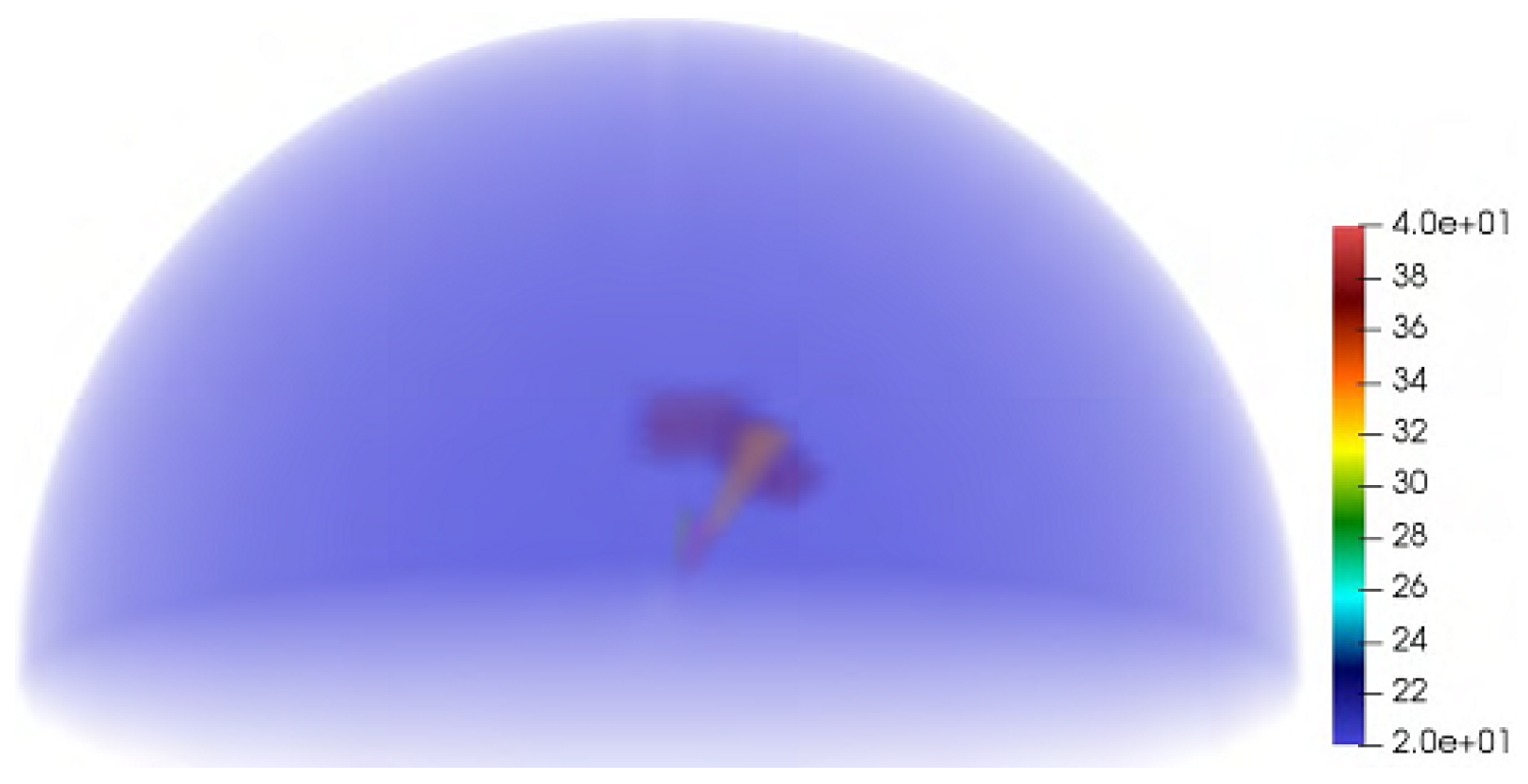
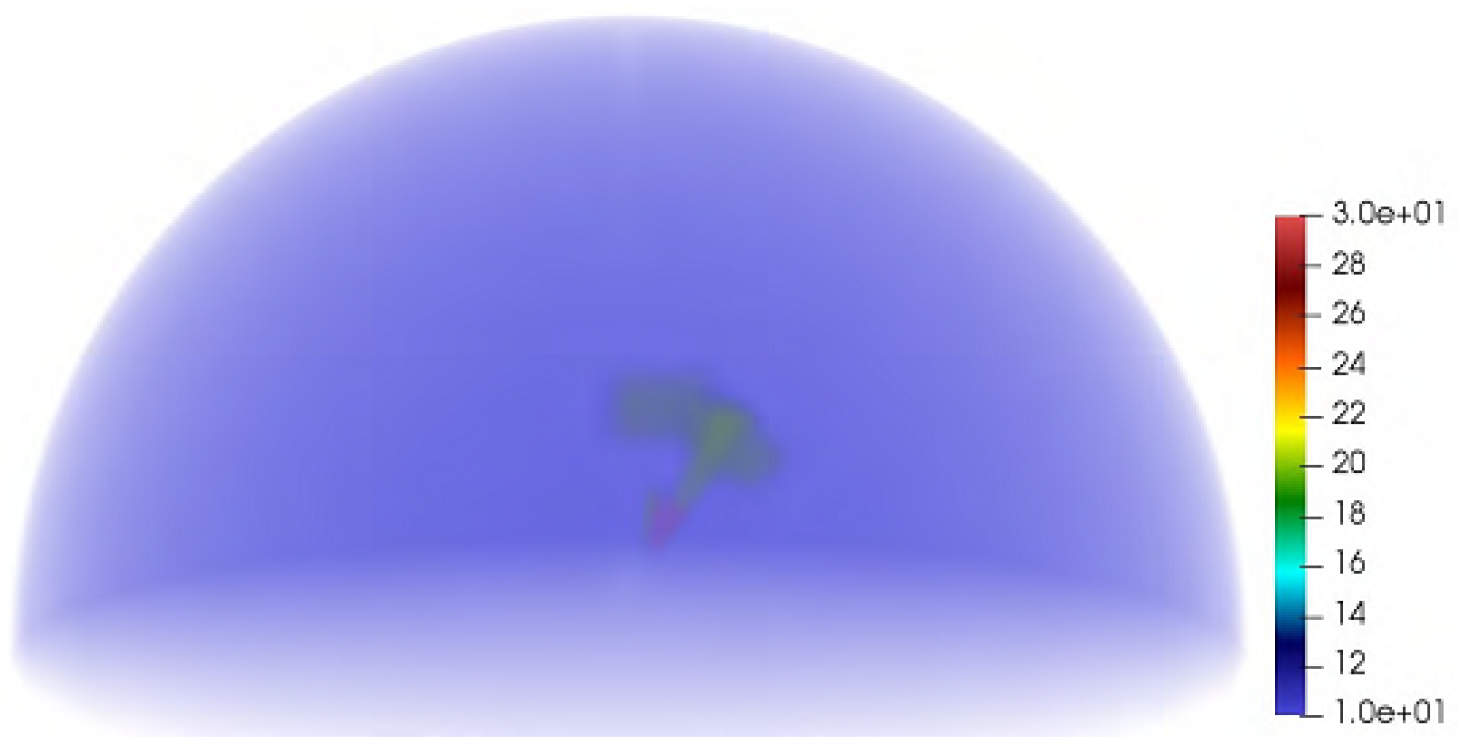
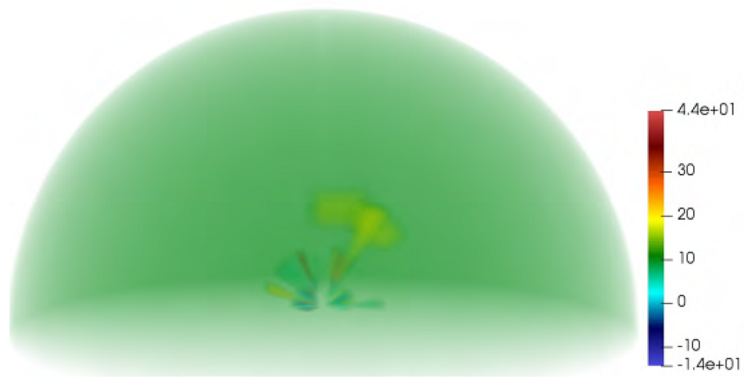
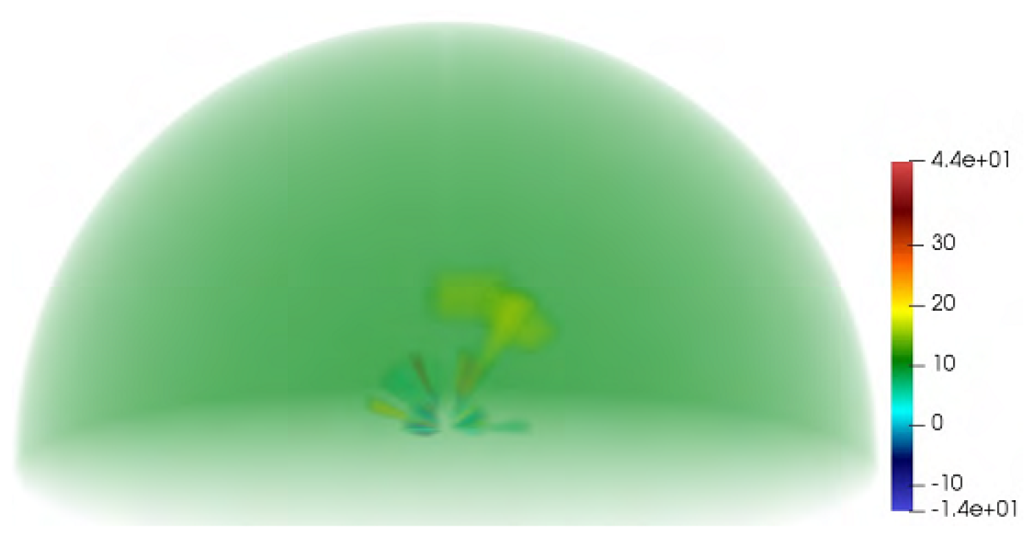
The following section presents an example of the results of solutions to the inverse problem using the developed two-step method. The chosen grid size is $12\times 12\times 12$ with a frequency of 100 GHz, and the hemisphere has a radius of 15 cm. The field source is located 5 cm above the hemisphere’s pole. The observation points where the field is measured are distributed around the body, with the closest point at a distance of about 1 cm from the hemisphere. The function ${\epsilon }_r\left(x\right)$ is complex-valued.

From Figure 1, Figure 2, Figure 3 and Figure 4, it is evident that the inhomogeneity is detected and correctly localized. However, the shape of the inhomogeneity and the values of the permittivity differ somewhat from the original data. Further refinement of the solution is possible by increasing the set of the initial data and refining the mesh.

Figure 1. Exact solution: real part ${\epsilon }_r\left(x\right)$.

Figure 2. Exact solution: imaginary part ${\epsilon }_r\left(x\right)$.

Figure 3. Approximate solution: real part ${\epsilon }_r\left(x\right)$.

Figure 4. Approximate solution: imaginary part ${\epsilon }_r\left(x\right)$.

7. Discussion and Conclusions

This paper has developed and justified a two-step method for reconstructing the permittivity of an inhomogeneous body having the shape of a hemisphere from near-field measurements based on solving a vector linear integro-differential equation in the inhomogeneity domain. A numerical method for solving the inverse problem is proposed. The computational experiments conducted confirm the effectiveness of the proposed algorithm for solving the inverse diffraction problem.

Note that in inverse problems, the accuracy of computations at all stages of the solution plays a decisive role. Additionally, preprocessing of input data is necessary, which filters out white noise and systematic measurement errors. This paper does not discuss the preprocessing of input data.

In the proposed method of solving the problem, the basis functions are chosen so as to allow the divergence operation to be moved under the integral sign, transferred to the basis function, and computed analytically. This reduces the number of computations, leading to errors due to rounding. Moreover, it becomes possible to move the gradient operation under the integral sign since the singularity becomes integrable. This also reduces computational errors.

Thus, the proposed method for solving the inverse problem achieves an acceptable practical error using a relatively small number of measurements and solving on a coarse grid. This issue becomes particularly important in practice when it is difficult to conduct a large number of measurements.

The two-step method for solving the inverse problem of detecting inhomogeneities in a dielectric body of arbitrary shape based on near-field measurements was proposed and substantiated in [8,9,10,11,12]. In these works, in particular, the uniqueness of the solution to the inverse problem (using the formulation considered in this article) has been proven, i.e., the existence and uniqueness of the solution to the system of linear algebraic equations. Note that proofs of the uniqueness of the solution in inverse problem studies are relatively rare. In our case, the problem formulation was initially chosen to be finite-dimensional (we are searching for a finite number of unknown parameters, namely, the values of dielectric permittivity at the grid elements). The results of calculations have been presented for the two-dimensional (2D) [9] and three-dimensional (3D) scalar inverse problems [8,9,10] as well as for a 3D vector inverse problem [11] on a parallelepiped, and for an N-dimensional scalar inverse problem [12]. In this work, we apply and develop the two-step method for solving the inverse problem on a hemispherically shaped body in spherical coordinates, which has certain peculiarities, addressed in detail in our study. Numerical results are also presented for determining inhomogeneities in the hemisphere.