Effects of Anisotropy, Convection, and Relaxation on Nonlinear Reaction-Diffusion Systems

Abstract

The effects of relaxation, convection, and anisotropy on a two-dimensional, two-equation system of nonlinearly coupled, second-order hyperbolic, advection–reaction–diffusion equations are studied numerically by means of a three-time-level linearized finite difference method. The formulation utilizes a frame-indifferent constitutive equation for the heat and mass diffusion fluxes, taking into account the tensorial character of the thermal diffusivity of heat and mass diffusion. This approach results in a large system of linear algebraic equations at each time level. It is shown that the effects of relaxation are small although they may be noticeable initially if the relaxation times are smaller than the characteristic residence, diffusion, and reaction times. It is also shown that the anisotropy associated with one of the dependent variables does not have an important role in the reaction wave dynamics, whereas the anisotropy of the other dependent variable results in transitions from spiral waves to either large or small curvature reaction fronts. Convection is found to play an important role in the reaction front dynamics depending on the vortex circulation and radius and the anisotropy of the two dependent variables. For clockwise-rotating vortices of large diameter, patterns similar to those observed in planar mixing layers have been found for anisotropic diffusion tensors.

1. Introduction

Most of the heat and mass transfer phenomena that arise in science and engineering are usually modeled by means of the well-known Fourier and Fick’s second laws, respectively, whereby the heat and mass transfer fluxes are assumed to be linearly proportional to the temperature and concentration gradients, respectively, and the proportionality is, in many cases, assumed to be a scalar rather than a tensor. The application of these laws to problems where the length scales are small, e.g., microfluidics, and/or the heat and mass flux are very large and may not be valid because these laws result in parabolic partial differential equations characterized by an infinite speed of propagation, and delays may occur between, say, the time at which the temperature gradient is imposed and the time at which the heat flux is observed. This delay was usually taken care of in the past by the well-known linear relaxation equation [1]:

$${\displaystyle \frac{dq}{dt}}=-{\displaystyle \frac{1}{\tau }}(q-q_e),$$

(1)

where $q\left(t\right)$ denotes a variable that depends on time t, $q_e$ is its equilibrium value and $\tau$ is the relaxation time, which may also be considered as a delay time.

The solution to the above equation is as follows:

$$q\left(t\right)=q_e+(q\left(0\right)-q_e)exp\left(-{\displaystyle \frac{t}{\tau }}\right),$$

(2)

which indicates that the equilibrium value/state is reached in an exponential manner.

Although linear Equation (1) has been frequently used in the past in fluid dynamics, acoustics, heat, and mass transfer [2,3], high-temperature phenomena, biology [4], epidemiology, population dynamics, reaction-diffusion systems [5], thermoelasticity [6], etc., it suffers from several problems. First, its use may result in a violation of the second law of thermodynamics [7]. Second, although its use may be somewhat justified when macroscopic variables only depend on time, there remains the question about the time-derivative that should appear in that equation in moving media [1,8,9]. Third, in moving media, the use of either a partial derivative with respect to time or a material/substantial time derivative does not satisfy the principle of frame-indifference of continuum mechanics [10].

It is interesting to note that the above linear relaxation equation may be written as $q+\tau {\displaystyle \frac{dq}{dt}}=q_e$ which reminds the reader of the Maxwell–Cattaneo–Vernotte constitutive law [2,11] (cf. Section 2).

As stated above, in many applications of Fourier and Fick laws in heat and mass transfer problems, thermal conductivity, and mass diffusion tensors are assumed to be isotropic and, in many cases are considered to be proportional to the unity or identity tensor. As a consequence, terms associated with the presence of second-order mixed derivatives and cross-diffusion are ignored, even though they are known to play some role in combustion phenomena, e.g., Soret and Dufour, thermodiffusion, barodiffusion, etc. [12]. In particular, cross-diffusion in two-equation, two-dimensional systems of parabolic reaction-diffusion is known to play a paramount role in determining pattern formation and stability, e.g., [13,14]. However, the effects of second-order mixed derivatives on either parabolic or hyperbolic, multi-dimensional advection–reaction–diffusion equations have not received much attention, presumably because these mixed terms couple the two directions of space.

In this paper, we present a numerical study of a two-equation, two-dimensional, nonlinear system of advection–reaction–diffusion equations that accounts for the presence of two relaxation times and the anisotropy of the diffusion tensors in a convective environment.

The formulation and numerical methods presented in this paper apply not only to models of nonlinear heat and mass transfer phenomena where relaxation, advection, anisotropy, and chemistry result in second-order hyperbolic, advection–reaction–diffusion equations, they are also applicable to other models governed by the same type of equations that might be employed in the study and analysis of biological, ecological, epidemiological, etc., processes or systems.

This paper has been arranged as follows. In Section 2, the Maxwell–Cattaneo–Vernotte constitutive law for heat conduction and two constitutive models based on the use of the material or substantial derivative and Christov’s frame-indifference model is presented for a single dependent variable in order to emphasize their similarities and differences and point out which constitutive law for heat conduction may be formulated for either only the temperature or both the temperature and the heat flux. In the same section, the one-equation formulation is extended to deal with several dependent variables for the case that the (heat and mass) diffusion fluxes are given by Christov’s constitutive model. The numerical method employed in the simulations is presented in Section 4. A summary of a large set of numerical experiments that have been performed for different relaxation times, velocity fields, and coefficients that multiply the second-order mixed-diffusion terms is presented in Section 5. The final section summarizes some of the most common findings on the effects of the anisotropy of diffusion tensors, relaxation time, and velocity field on second-order hyperbolic, advection–reaction–diffusion models of heat and mass transfer and other phenomena described in the manuscript.

2. Formulation

As stated in the introduction, for the sake of clarity, in this section, we first present and compare three constitutive laws for the conduction heat flux that account for relaxation for a single dependent variable. The one-variable formulation is then extended to several variables.

2.1. One-Variable Formulation

In this subsection, we consider the following, time-dependent, multi-dimensional, nonlinear reaction-diffusion equation:

$$\rho c{\displaystyle \frac{DT}{Dt}}=-\nabla ·\mathbf{q}+S,t>0,\mathbf{x}\in \mathsf{\Omega },$$

(3)

where $\rho$ and c denote the mass density and specific heat, respectively, which may depend on T, t is time, T denotes the temperature, S is a (nonlinear) source or reaction term, which may depend on t, $\mathbf{x}$, and T; $\mathbf{q}$ is the conduction heat flux vector, $\mathbf{x}$ and $\mathsf{\Omega }$ denote the spatial coordinates and domain, respectively, ${\displaystyle \frac{DT}{Dt}}=T_t+\mathbf{v}·\nabla T$ is the material or substantial derivative, the subscripts denote partial differentiation, and $\mathbf{v}$ is the velocity vector.

When Fourier’s law is applicable [15], $\mathbf{q}(t,\mathbf{x})=-\mathbf{K}\nabla T(t,\mathbf{x})$, where $\mathbf{K}$ denotes the positive definite thermal conductivity tensor. Fourier’s law assumes that a temperature gradient at $(t,\mathbf{x})$ results in a heat flux at the same location and time; conversely, it also indicates that a heat flux at $(t,\mathbf{x})$ results in a temperature gradient at the same location and time.

The use of Fourier’s law in Equation (3) yields the following well-known parabolic equation for T:

$$\rho c{\displaystyle \frac{DT}{Dt}}=\nabla ·(\mathbf{K}\nabla T)+S,$$

(4)

which is characterized by an infinite speed of propagation and contains only the temperature.

Equation (4) is subject to the initial condition $T(0,\mathbf{x})=T_0\left(\mathbf{x}\right)$ and boundary conditions at the domain boundaries, i.e., on $\partial \mathsf{\Omega }$. For Dirichlet’s boundary conditions, $T(t,{\mathbf{x}}_b)=\varphi \left(t\right)$, where ${\mathbf{x}}_b$ denotes the spatial coordinates of the boundary and $\varphi \left(t\right)$ is the boundary temperature. For the Neumann boundary conditions, $\mathbf{q}(t,{\mathbf{x}}_b)·\mathbf{n}=\theta \left(t\right)$, where $\mathbf{n}$ is the unit’s outward-pointing vector normal to the boundary $\partial \mathsf{\Omega }$ and $\theta \left(t\right)$ stands for the heat flux flowing out at the domain boundary. For Robin’s boundary conditions, $\mathbf{q}(t,{\mathbf{x}}_b)·\mathbf{n}=\psi (T(t,{\mathbf{x}}_b),T_{\infty })$, where $T_{\infty }$ denotes the temperature far away from the domain $\mathsf{\Omega }$.

For heat transfer phenomena occurring at the micro- or nanoscale or at very fast rates, it is well known that Fourier’s law is not valid. As indicated in the introduction, Maxwell, Cattaneo, and Vernotte assumed that a temperature gradient applied at t results in a heat flux at $t+\tau$, where $\tau$ is the relaxation time [2,3], i.e.,

$$\mathbf{q}(t+\tau ,\mathbf{x})=-\mathbf{K}\nabla T,$$

(5)

which together with Equation (3) provides a system of delay equations in time for T and $\mathbf{q}$.

A Taylor series expansion of Equation (5) up to $\mathcal{O}\left({\tau }^2\right)$ may be written as follows:

$$\mathbf{q}(t,\mathbf{x})+\tau {\mathbf{q}}_t(t,\mathbf{x})=-\mathbf{K}\nabla T.$$

(6)

By taking the divergence of Equation (6) and using Equation (3), one may easily obtain the following:

$$\rho c{\displaystyle \frac{DT}{Dt}}+\tau {\displaystyle \frac{\partial }{\partial t}}\left(\rho c{\displaystyle \frac{DT}{Dt}}\right)=\nabla ·(\mathbf{K}\nabla T)+S+\tau {\displaystyle \frac{\partial S}{\partial t}},$$

(7)

which is a nonlinear, second-order hyperbolic equation for T whose solutions have a finite speed of propagation. Equation (7) reduces to Equation (4) for $\tau =0$.

For heat conduction in moving media, it is clear that no information regarding the velocity field is explicitly included in Equation (6). However, if instead of Equation (6), one employs the following:

$$\mathbf{q}+\tau {\displaystyle \frac{D\mathbf{q}}{Dt}}=-\mathbf{K}\nabla T,$$

(8)

and then takes the divergence of this equation and makes use of Equation (3), it is easy to obtain the following:

$$\rho c{\displaystyle \frac{DT}{Dt}}+\tau {\displaystyle \frac{D}{Dt}}\left(\rho c{\displaystyle \frac{DT}{Dt}}\right)=\nabla ·(\mathbf{K}\nabla T)+S+\tau {\displaystyle \frac{DS}{Dt}}+\tau \nabla \mathbf{v}:\nabla \mathbf{q},$$

(9)

which clearly differs from Equation (7) in all the terms containing $\tau$, although it reduces to Equation (7) for $\tau =0$. Moreover, unless $\tau \nabla \mathbf{v}:\nabla \mathbf{q}$ is nil, Equation (9) contains both T and $\mathbf{q}$ and, therefore, Equations (8) and (9) are coupled and must be solved as a system of (coupled) equations (cf. compare Equations (7) and (9)). This is closely aligned with Christov’s frame-indifference formulation of the Maxwell–Cattaneo–Vernotte model of heat conduction [9], i.e.,

$$\mathbf{q}+\tau \left({\displaystyle \frac{D\mathbf{q}}{Dt}}-\mathbf{q}·\nabla \mathbf{v}+(\nabla ·\mathbf{v})\mathbf{q}\right)=-\mathbf{K}\nabla T,$$

(10)

whose divergence may be written as follows:

$$Q+\tau \left({\displaystyle \frac{DQ}{Dt}}+Q\nabla ·\mathbf{v}\right)=-\nabla ·(\mathbf{K}\nabla T),$$

(11)

where $Q\equiv \nabla \mathbf{q}$.

For solenoidal velocity fields, i.e., $\nabla ·\mathbf{v}=0$, the use of Q from Equation (3) into Equation (11) yields the following:

$$\rho c{\displaystyle \frac{DT}{Dt}}+\tau {\displaystyle \frac{D}{Dt}}\left(\rho c{\displaystyle \frac{DT}{Dt}}\right)=\nabla ·(\mathbf{K}\nabla T)+S+\tau {\displaystyle \frac{DS}{Dt}},$$

(12)

which differs from Equation (9) in that the latter contains a tensor contraction term, i.e., the last term on the right-hand side of Equation (9).

Equation (11) may also be written as follows:

$$Q+\tau \left({\displaystyle \frac{\partial Q}{\partial t}}+\nabla ·\left(\mathbf{v}Q\right)\right)=-\nabla ·(\mathbf{K}\nabla T),$$

(13)

which, upon obtaining Q from Equation (3) and substituting it in Equation (11), may be written as follows:

$$\rho c(1+\tau \nabla ·\mathbf{v}){\displaystyle \frac{DT}{Dt}}+\tau {\displaystyle \frac{D}{Dt}}\left(\rho c{\displaystyle \frac{DT}{Dt}}\right)=\nabla ·(\mathbf{K}\nabla T)+S+\tau \left({\displaystyle \frac{DS}{Dt}}+S\nabla ·\mathbf{v}\right),$$

(14)

which is a second-order hyperbolic equation for T, which has a finite speed of propagation and reduces to Equation (4) for $\tau =0$.

If $\rho c$ and $\mathbf{K}$ are constant and the velocity field is solenoidal, Equation (14) is as follows:

$$\rho c{\displaystyle \frac{DT}{Dt}}+\tau \rho c{\displaystyle \frac{D}{Dt}}\left({\displaystyle \frac{DT}{Dt}}\right)=\nabla ·(\mathbf{K}\nabla T)+S+\tau {\displaystyle \frac{DS}{Dt}},$$

(15)

which may also be written as follows:

$$\rho c\varphi +\tau \rho c{\displaystyle \frac{D\varphi }{Dt}}=\nabla ·(\mathbf{K}\nabla T)+S+\tau J\varphi ,$$

(16)

for $S=S\left(T\right)$, where $J={\displaystyle \frac{dS}{dT}}$ denotes the Jacobian of S, and $\varphi ={\displaystyle \frac{DT}{Dt}}$.

The positive definiteness of the thermal conductivity tensor in two dimensions requires that $K_{11}>0$, $K_{22}>0$ and $K_{11}{K}_{22}>K_{12}{K}_{21}$, where $K_{ij}$, $i=1,2$ and $j=1,2$, are the components of $\mathbf{K}$. Moreover, $\nabla ·(\mathbf{K}\nabla T)=K_{11}{T}_{xx}+(K_{12}+K_{21})T_{xy}+K_{22}{T}_{yy}$ in two dimensions, and exhibits anisotropy if $K_{11}\ne K_{22}$ even for $K_{12}=K_{21}=0$ or if either $K_{12}$ or $K_{21}$ is not nil.

The eigenvalues of the thermal conductivity tensor may be written as follows:

$$\lambda ={\displaystyle \frac{1}{2}}(K_{11}+K_{22})\pm \sqrt{{\displaystyle \frac{1}{4}}{(K_{11}-K_{22})}^2+K_{12}{K}_{21}},$$

(17)

are both positive on account of the positive definiteness of the thermal conductivity tensor and may be used to estimate the speed of propagation of Equations (7), (9), or (12), as follows.

For a one-dimensional problem with constant heat capacity, i.e., constant $\rho c$, constant velocity v and constant thermal conductivity, these equations may be written as follows:

$$\rho c\tau T_{tt}+\rho cv{T}_{xt}-K{T}_{xx}=F(T,T_t,T_x),$$

(18)

where its right-hand side only depends on T and its first-order partial derivatives with respect to space and time.

Equation (18) is a linear, second-order, one-dimensional hyperbolic equation whose characteristic lines have slopes given by the following:

$${\displaystyle \frac{dx}{dt}}=-v\pm \sqrt{v^2+4{\displaystyle \frac{K}{\rho c\tau }}},$$

(19)

and indicate that there is propagation at finite speed for $\tau \ne 0$ in both directions of the x-axis. For $\tau =0$, Equation (19) indicates that the propagation speed is infinite, consistent with the fact that Equation (18) is parabolic when relaxation times are zero.

Estimates of the velocity of propagation in several dimensions may be obtained as $v_{th}=\sqrt{{\displaystyle \frac{K}{\rho c\tau }}}$, which depends on the thermal diffusivity and relaxation time and increases as the relaxation time increases. This velocity estimate is usually larger than $\left|\mathbf{v}\right|$ in microfluidics and fast heat transfer phenomena at the microscale and nanoscale; however, $v_{th}$ may be of the same order of magnitude as or even smaller than v in various models, including biological [4], epidemiological [16,17], virus infection [18], forest fire [19], ecological [20], chemistry [21,22,23], chemical engineering [24], etc.

Using $v_{th}$, Equation (19) may be written as follows:

$${\displaystyle \frac{dx}{dt}}=-v\pm \sqrt{v^2+4v_{th}^2},$$

which indicates that ${\displaystyle \frac{dx}{dt}}\approx \pm 2v_{th}$ for $v_{th}>>\left|v\right|$.

2.2. Multi–Variable Formulation

The formulation presented in the previous section has been generalized for coupled heat and mass transfer problems where there is relaxation for both the temperature and the species concentration; in addition, the thermal and mass diffusion coefficients are tensors. This generalization can also be applied to various models, including biological [4], epidemiological [16,17], virus infection [18], ecological [20], chemical [24], etc., which are characterized by second-order hyperbolic, nonlinear advection–reaction–diffusion equations. It reduces to the reaction-diffusion case when the relaxation times or inertia are negligible, and includes both isotropic and anisotropic diffusion tensors, but does not account for cross-diffusion effects.

For several dependent variables, i.e., $Y^m$, $m=1,2,\cdots ,NV$, where $NV$ is the number of dependent variables, and constants $\rho c$ and $\mathbf{K}$, the nondimensional form of Equation (14) may be written as follows:

$$(1+{\tau }^m\nabla ·\mathbf{v}){\displaystyle \frac{D{Y}^m}{Dt}}+{\tau }^m{\displaystyle \frac{D}{Dt}}\left({\displaystyle \frac{D{Y}^m}{Dt}}\right)=\nabla ·({\mathbf{K}}^m\nabla Y^m)+S^m+{\tau }^m\left({\displaystyle \frac{D{S}^m}{Dt}}+S^m\nabla ·\mathbf{v}\right),$$

(20)

where $Y^m$ denotes the m-th dependent variable characterized by a relaxation time ${\tau }^m$, a source term $S^m$, and a diffusivity tensor ${\mathbf{K}}^m$.

Equation (20) corresponds to the Christov’s frame-indifferent constitutive equations [9] for the diffusion fluxes of all dependent variables, and does not take cross-diffusion effects into account, i.e., the effects of $\nabla Y^m$ into the equation for $Y^l$ for $m\ne l$.

Equation (20) is subject to $Y^m(0,\mathbf{x})=G^m\left(\mathbf{x}\right)$ and ${\displaystyle \frac{\partial Y^m}{\partial t}}(0,\mathbf{x})=H^m\left(\mathbf{x}\right)$, where $G^m$ and $H^m$ are functions of space. For homogeneous Neumann boundary conditions, i.e., $\mathbf{n}·\nabla Y^m=0$ at $\partial \mathsf{\Omega }$, where $\mathbf{n}$ denotes the unit vector normal to the boundary.

3. Numerical Method

In two dimensions, the domain $[-A,A]\times [-B,B]$, where $2A$ and $2B$ denote the sides of the rectangular domain, was discretized in equally spaced grids consisting of $NX=NI+1$ and $NY=NJ+1$ points in the x- and y-directions, respectively, so that the grid spacings in those directions are $\mathsf{\Delta }x={\displaystyle \frac{2A}{NI}}$ and $\mathsf{\Delta }y={\displaystyle \frac{2B}{NJ}}$, respectively.

The second-order spatial derivatives that appear in the diffusion term in Equation (20), i.e., ${\left(Y^m\right)}_{xx}$, ${\left(Y^m\right)}_{xy}$, and ${\left(Y^m\right)}_{yy}$, were discretized by means of the well-known, second-order accurate, central difference formulae, whereas the first-order spatial derivatives were discretized by means of either first-order accurate upwind differences or second-order accurate central differences depending on whether the absolute value of the local mesh Péclet number was greater than, less than, or equal to two, respectively.

The spatial discretization discussed in the previous paragraph results in the following systems of second-order, nonlinear ordinary differential equations:

$${\mathbf{M}}_{ij}{\displaystyle \frac{d^2{\mathbf{U}}_{ij}}{d{t}^2}}+{\mathbf{D}}_{ij}{\displaystyle \frac{d{\mathbf{U}}_{ij}}{dt}}={\mathbf{F}}_{ij}(x_i,y_j,{\mathbf{V}}_{ij}),$$

(21)

where $\mathbf{U}={(Y^1,Y^2,\cdots ,Y^{NV})}^T$, the superscript T represents transpose, and the subscript $ij$ indicates the $(i,j)$ grid point. ${\mathbf{V}}_{ij}$ depends on ${\mathbf{U}}_{MN}$, where $i-1\le M\le i+1$, and $j-1\le N\le j+1$. The right-hand side of Equation (21) is a nonlinear function owing to the nonlinear dependence of the source terms of Equation (20) on $Y^m$.

The components of the mass and damping matrices, i.e., ${\mathbf{M}}_{ij}$ and ${\mathbf{D}}_{ij}$, respectively, and ${\mathbf{F}}_{ij}$ that appear in Equation (21) may be easily deduced from the spatial discretization of Equation (20), but are not reported here.

Assembling Equation (21) for all the grid points—including those at the boundaries where second-order accurate discretizations were used for the first-order spatial derivatives that appeared in the homogeneous boundary conditions—results in the following system:

$$\mathcal{M}{\displaystyle \frac{d^2\mathcal{U}}{d{t}^2}}+\mathcal{D}{\displaystyle \frac{d\mathcal{U}}{dt}}=\mathcal{F}(\mathcal{U}).$$

(22)

Equation (22) was first discretized as follows:

$${\displaystyle \frac{1}{\mathsf{\Delta }{t}^2}}{\mathcal{M}}^n({\mathcal{U}}^{n+1}-2{\mathcal{U}}^n+{\mathcal{U}}^{n-1})+{\displaystyle \frac{1}{2\mathsf{\Delta }t}}({\mathcal{U}}^{n+1}-{\mathcal{U}}^{n-1})={\displaystyle \frac{1}{4}}({\mathcal{F}}^{n+1}+2{\mathcal{F}}^n+{\mathcal{F}}^{n-1}),$$

(23)

where the superscript n denotes the n-th time level, with $t^n=n\mathsf{\Delta }t$, $n=0,1,2,\cdots$, and $\mathsf{\Delta }t$ is the time step.

Equation (23) is second-order accurate in time [25] and represents $NX\times NY$ nonlinear equations, whose solution may be obtained through iterative techniques. However, by linearizing ${\mathcal{F}}^{n+1}$ about the n-th time level, i.e., ${\mathcal{F}}^{n+1}={\mathcal{F}}^n+{\mathcal{J}}^n({\mathcal{U}}^n-{\mathcal{U}}^n)+\mathcal{O}\left(\mathsf{\Delta }{t}^2\right)$, where ${\mathcal{J}}^n={\displaystyle \frac{\partial {\mathcal{F}}^n}{{\mathcal{U}}^n}}$ denotes the Jacobian matrix of $\mathcal{F}$, and neglecting the $\mathcal{O}\left(\mathsf{\Delta }{t}^2\right)$, Equation (23) may be written as the following system of linear algebraic equations:

$${\mathcal{P}}^n{\mathcal{U}}^{n+1}={\mathcal{Q}}^n,$$

(24)

where

$${\mathcal{P}}^n={\mathcal{M}}^n+{\displaystyle \frac{\mathsf{\Delta }t}{2}}{\mathcal{D}}^n-{\displaystyle \frac{\mathsf{\Delta }{t}^2}{4}}{\mathcal{J}}^n,$$

(25)

$${\mathcal{Q}}^n={\mathcal{M}}^n(2{\mathcal{U}}^n-{\mathcal{U}}^{n-1})+{\displaystyle \frac{\mathsf{\Delta }t}{2}}{\mathcal{D}}^n{\mathcal{U}}^n+{\displaystyle \frac{\mathsf{\Delta }{t}^2}{4}}(3{\mathcal{F}}^n+{\mathcal{F}}^{n-1}-{\mathcal{J}}^n{\mathcal{U}}^n),$$

(26)

are both sparse matrices.

Equation (24) was solved by means of a Krylov space method [26,27,28,29] for non-symmetric systems when upwind differences were employed to discretize the first-order spatial derivatives that appear in Equation (20). A Krylov space method for symmetric systems was used when the mesh Péclet number was less than or equal to two and the advection terms were discretized by means of second-order, central differences.

Accuracy Assessment

The accuracy of the time-linearized, three-time-level method described above was first assessed by comparing the numerical results with the exact solution of the following (scalar) equation:

$$\tau u_{tt}+\alpha u_t=D{u}_{xx}+E{u}_{yy}+S\left(u\right),0<x<a,0<y<b,t>0,$$

(27)

subject to homogeneous Dirichlet boundary conditions, as follows:

$$u(t,0,y)=u(t,a,y)=0,u(t,x,0)=u(t,x,b)=0,$$

(28)

and

$$u(0,x,y)=sin\left({\displaystyle \frac{\pi x}{a}}\right)sin\left({\displaystyle \frac{\pi y}{b}}\right),$$

(29)

where $S\left(u\right)=\gamma u$, $\tau \ge 0$, $\alpha \ge 0$, $D\ge 0$, $E\ge 0$ and $\gamma \le 0$ are constants.

The solution of Equation (27) subject to Equations (28) and (29) may be written as follows:

$$u_{ex}(t,x,y)=\varphi \left(t\right)sin\left({\displaystyle \frac{\pi x}{a}}\right)sin\left({\displaystyle \frac{\pi y}{b}}\right),$$

(30)

where

$$\begin{array}{cc}\hfill & \varphi \left(t\right)=exp\left(-{\displaystyle \frac{\alpha t}{2\tau }}\right)\mathrm{for}\tau ={\tau }_{cr},\hfill \end{array}$$

(31)

$$\begin{array}{cc}\hfill & \varphi \left(t\right)=exp\left(-{\displaystyle \frac{\alpha t}{2\tau }}\right)cosh\left({\displaystyle \frac{\alpha t}{2\tau }}\mathsf{\Omega }\right)\mathrm{for}\tau <{\tau }_{cr},\hfill \end{array}$$

(32)

$$\begin{array}{cc}\hfill & \varphi \left(t\right)=exp\left(-{\displaystyle \frac{\alpha t}{2\tau }}\right)cos\left({\displaystyle \frac{\alpha t}{2\tau }}\omega \right)\mathrm{for}\tau >{\tau }_{cr},\hfill \end{array}$$

(33)

the subscript $ex$ stands for exact solution, ${\tau }_{cr}={\alpha }^2/\left(4\left(D{\displaystyle \frac{{\pi }^2}{a^2}}+E{\displaystyle \frac{{\pi }^2}{b^2}}-\gamma \right)\right)$ denotes the critical relaxation time, $\mathsf{\Omega }=\sqrt{1-{\displaystyle \frac{\tau }{{\tau }_{cr}}}}$ and $\omega =\sqrt{{\displaystyle \frac{\tau }{{\tau }_{cr}}}-1}$.

The critical relaxation time decreases as the diffusion coefficients in the x- and/or y-directions increase, is nil when $\alpha =0$, i.e., in the absence of temporal damping, and decreases as the absolute value of the reaction increases. (Recall that $\gamma \le 0$).

The order of convergence of the numerical method presented above for Equation (27) is determined as follows. For a time step equal to k and grid spacings in the x- and y-directions equal to h and H, respectively, the numerical solution may be written as follows:

$$u_{(k,h,h)}(t^n,x_i,y_j)=u_{ex}(t^n,x_i,y_j)+C{k}^p+F{h}^q+G{H}^r,$$

(34)

where $t^n$ denotes the n-th time level, and $x_i$ and $y_j$ stand for the x- and y-coordinates of the $(i,j)$-the grid point, and, therefore, the values of p, q, and r may be easily deduced by obtaining numerical solutions with $k/2$ and $k/4$, $h/2$, and $h/4$, and H and $H/2$, respectively, as follows:

$$p={\displaystyle \frac{1}{log2}}log\left|{\displaystyle \frac{u_{(k,h,H)}(t^n,x_i,y_j)-u_{(k/2,h,H)}(t^n,x_i,y_j)}{u_{(k/2,h,H)}(t^n,x_i,y_j)-u_{(k/4,h,H)}(t^n,x_i,y_j)}}\right|,$$

(35)

$$q={\displaystyle \frac{1}{log2}}log\left|{\displaystyle \frac{u_{(k,h,H)}(t^n,x_i,y_j)-u_{(k,h/2,H)}(t^n,x_i,y_j))}{u_{(k,h/2,H)}(t^n,x_i,y_j)-u_{(k,h/4,H)}(t^n,x_i,y_j)}}\right|,$$

(36)

and

$$r={\displaystyle \frac{1}{log2}}log\left|{\displaystyle \frac{u_{(k,h,H)}(t^n,x_i,y_j)-u_{(k,h,H/2)}(t^n,x_i,y_j))}{u_{(k,h,H/2)}(t^n,x_i,y_j)-u_{(k,h,H/4)}(t^n,x_i,y_j)}}\right|,$$

(37)

respectively, where it is understood that the differences that appear on the right-hand sides of Equations (35)–(37) are taken at the same locations and times.

Once the values of p, q, and r are obtained as indicated above, those of C, F, and G may be easily obtained from the numerical solutions corresponding to k and $k/2$, h and $h/2$, and H and $H/2$, respectively, but are not shown here.

It must be noted that Equation (34) is really an asymptotic approximation whose temporal and spatial errors correspond to the last three terms on the the right-hand side of that equation. This means that, owing to the discretization in both space and time, p, q, C, F, and G might depend on k, h, and H and $t^n$, $x_i$, and $y_j$, if the time step and grid spacings are not small enough. When this occurs, it is convenient to replace the absolute values of the numerators and denominators that appear on the right-hand sides of Equations (35)–(37) with their discrete $L_2$, $L_1$, or $L_{\infty }$ norms. For example, $|u_{(k,h,H)}(t^n,x_i,y_j)-u_{(k/2,h,H)}(t^n,x_i,y_j)|$ is replaced with the following:

$$\sqrt{{\displaystyle \frac{1}{NX}}{\displaystyle \frac{1}{NY}}\sum _{i=1}^{NX}\sum _{j=1}^{NY}{\left(u_{(k,h,h)}(t^n,x_i,y_j)-u_{(k/2,h,H)}(t^n,x_i,y_j))\right)}^2},$$

(38)

$${\displaystyle \frac{1}{NX}}{\displaystyle \frac{1}{NY}}\sum _{i=1}^{NX}\sum _{j=1}^{NY}|u_{(k,h,H)}(t^n,x_i,y_j)-u_{(k/2,h,H)}(t^n,x_i,y_j)|,$$

(39)

or

$$\underset{1\le i\le NX,1\le j\le NY}{max}|u_{(k,h,H)}(t^n,x_i,y_j)-u_{(k/2,h,H)}(t^n,x_i,y_j)|,$$

(40)

respectively.

For $\alpha =D=E=a=b=1$, $\gamma =0$ and $\tau ={\displaystyle \frac{{\tau }_{cr}}{10}}$, numerical experiments performed with $\mathsf{\Delta }t=k=0.1$, 0.01, and 0.001, and $NX=NY=41$ and 401, show that at $t=0.8$, $p=2.13$ and $q=1.98$, which are consistent with second-order accuracies in both space and time of the numerical method; ${max}_{1\le i\le 401,1\le j\le 401}|u_{(0.001,0.0025,0.0025)}(0.8,x_i,y_j)-u_{ex}(0.8,x_i,y_j)|=0.7534\times {10}^{-6}$ and it occurs at $i=j=201$. For the same values of the parameters just mentioned, except for $\gamma =-1$, there is a linear reaction term, and it was found that, at $t=0.8$, $p=2.19$, $q=2.04$, and ${max}_{1\le i\le 401,1\le j\le 401}|u_{(0.001,0.0025,0.0025)}(0.8,x_i,y_j)-u_{ex}(0.8,x_i,y_j)|=0.6389\times {10}^{-6}$, occurring at $i=j=201$.

Similar results to those described in the previous paragraph have also been found in numerical experiments for $\tau ={\tau }_{cr}$ and $\tau =10{\tau }_{cr}$, $\alpha =D=E=a=b=1$, and $\gamma =0$ and $-1$. For example, for $\gamma =-1$ and $\tau ={\tau }_{cr}$, $p=2.02$, $q=1.94$, and ${max}_{1\le i\le 401,1\le j\le 401}|u_{(0.001,0.0025,0.0025)}$$(0.8,x_i,y_j)-u_{ex}(0.8,x_i,y_j)|=0.9809\times {10}^{-6}$, while, for $\gamma =-1$ and $\tau ={\tau }_{cr}$, $p=1.97$, $q=1.88$ and ${max}_{1\le i\le 401,1\le j\le 401}|u_{(0.001,0.0025,0.0025)}(0.8,x_i,y_j)-$$u_{ex}(0.8,x_i,y_j)|=1.1105\times {10}^{-6}$. This indicates that the temporal and spatial orders of convergence decrease slightly whereas the error slightly increases as the relaxation time is increased from subcritical to critical and then supercritical values. This should not come as a surprise since, as stated at the beginning of this subsection, supercritical relaxation times are characterized by a trigonometric dependence on time (cf. Equation (33)), which results in damped oscillatory solutions. On the other hand, a comparison between Equations (31) and (32) indicates that since the hyperbolic cosine is larger than one, supercritical relaxation times result in monotonically decreasing solutions that are less damped than those corresponding to the critical relaxation time.

Numerical experiments were also performed with nonlinear source terms, e.g., $S\left(u\right)=u(1-u)$ in Equation (27), for which no analytical solution is available with and without velocity fields. In such cases, the accuracies of the numerical solutions were assessed by determining both the orders of convergence in time and space, i.e., p, q, and r, respectively, as in Equations (35)–(37), respectively, and $E_{k,h,H}^t\equiv {max}_{1\le i\le NI,1\le j\le NJ}|u_{(k,h,H)}(t^n,x_i,y_j)-u_{(k/2,h,H)}(t^n,x_i,y_j)|$, $E_{k,h,H}^x\equiv {max}_{1\le i\le NI,1\le j\le NJ}|u_{(k,h/2,H)}(t^n,x_i,y_j)-u_{(k,h,H)}(t^n,x_i,y_j)|$, and $E_{k,h,H}^y\equiv {max}_{1\le i\le NI,1\le j\le NJ}|u_{(k,h,H/2)}(t^n,x_i,y_j)-u_{(k,h,H)}(t^n,x_i,y_j)|$, which denote the differences in the numerical solutions obtained with time steps equal to k and $k/2$, grid spacings in the x-directions equal to h and $h/2$, and grid spacings in the y-direction equal to H and $H/2$, respectively. The time step and grid spacings were considered to be adequate and, therefore, the solution was considered to be accurate and acceptable whenever $E_{k,h,H}^t\le {10}^{-4}$, $E_{k,h,H}^x\le {10}^{-4}$ and $E_{k,h,H}^y\le {10}^{-4}$ were satisfied.

For the results presented in the next section, the convergence of the Krylov space method used to solve Equation (24) was set to ${10}^{-6}$, and the time step and grid spacings were determined by trial ande erroor until $E_{k,h,H}^t$, $E_{k,h,H}^x$, and $E_{k,h,H}^y$ were less than or equal to ${10}^{-4}$, $5\times {10}^{-4}$ and $5\times {10}^{-4}$, respectively, for $t\le 100$.

4. Results

The multi-dimensional formulation presented in Section 2.2 has been applied to a two-equation, two-dimensional problem characterized by the following: $u\equiv Y^1$, $v\equiv Y^2$, ${\tau }_u\equiv {\tau }^1$, ${\tau }_v\equiv {\tau }^2$, ${\mathbf{D}}^u\equiv {\mathbf{K}}^1$, $D_{11}^u=D_{22}^u=1$, $D_{12}\equiv D_{12}^u+D_{21}^u$, ${\mathbf{D}}^v\equiv {\mathbf{K}}^2$, $D_{11}^v=D_{22}^v=0.6$, $d_{12}\equiv D_{12}^v+D_{21}^v$,

$$S_u={\displaystyle \frac{1}{ϵ}}\left(u-u^2-fv{\displaystyle \frac{u-q}{u+q}}\right),S_v=u-v,$$

(41)

and a time-independent velocity field corresponding to a Rankine vortex whose azimuthal velocity component is as follows:

$$u_{\theta }={\displaystyle \frac{\mathsf{\Gamma }}{2\pi }}{\displaystyle \frac{r}{R^2}}\mathrm{for}r\le R,u_{\theta }={\displaystyle \frac{\mathsf{\Gamma }}{2\pi r}}\mathrm{for}r>R,$$

(42)

$ϵ=0.01$, $f=1.4$, $q=0.002$, the subscripts u and v refer to the dependent variables $u(t,x,y)$ and $v(t,x,y)$, respectively, and $\mathsf{\Gamma }$ and R denote the circulation and core radius of the vortex, respectively. The velocity field in Cartesian coordinates is given by $\mathbf{v}=(U,V)$, where U and V are the velocity components in the x- and y-directions, respectively, which may be easily obtained from the azimuthal velocity component of Equation (42). Positive values of $\mathsf{\Gamma }$ or $\omega$ correspond to counter-clockwise rotating velocity fields.

For $\mathsf{\Gamma }=D_{12}=d_{12}={\tau }_u={\tau }_v=0$, i.e., in the absence of convection and with isotropic constant diffusion tensors for u and v, it is known that the two-equation system considered in this study has constant-period counter-rotating spiral wave solutions [30]. Therefore, a comparison of these solutions with those obtained with relaxation times ${\tau }_u\ne 0$ and/or ${\tau }_v\ne 0$, non-zero velocity fields $\mathbf{v}\ne \mathbf{0}$, and mixed diffusion terms $D_{12}\ne 0$ and/or $d_{12}\ne 0$, will allow us to determine the effects of these parameters on wave propagation.

Equation (20), as well as Equations (41) and (42), were solved in a square domain $[-L,L]\times [-L,L]$ with $L=7.5$, and the numerical method presented in Section 3, using equally spaced meshes consisting of, at least, $101\times 101$ grid points and a time step less or equal to $0.0001$, homogeneous Neumann conditions, and initial conditions identical to those employed in other studies [30]. Since the numerical method presented in Section 3 is second-order accurate in time and second-order accurate in space if the local Péclet number is less than or equal to two, the temporal discretization errors are much smaller than the spatial ones for the numerical experiments reported here. In addition, $\mathsf{\Delta }t<max({\tau }_u,{\tau }_v)$.

Since Equation (23) contains three time levels, the numerical method presented in Section 3 is not self-starting. In order to start the method, the value of ${\mathcal{U}}^1$, i.e., $\mathcal{U}\left(\mathsf{\Delta }t\right)$, must be given. This value may be obtained from the following Taylor series expansion:

$$\mathcal{U}\left(\mathsf{\Delta }t\right)=\mathcal{U}\left(0\right)+{\mathcal{U}}_t\left(0\right)\mathsf{\Delta }t+{\displaystyle \frac{1}{2}}{\mathcal{U}}_{tt}\left(0\right)\mathsf{\Delta }{t}^2+\mathcal{O}\left(\mathsf{\Delta }{t}^3\right),$$

(43)

where, as stated above, $\mathcal{U}\left(0\right)$ and ${\mathcal{U}}_t\left(0\right)$ are provided by the initial conditions, and ${\mathcal{U}}_{tt}\left(0\right)$ may be obtained by making use of Equation (20) at $t=0$.

Numerical experiments were performed to determine the effects of ${\tau }_u$ and ${\tau }_v$, $\omega \equiv {\displaystyle \frac{\mathsf{\Gamma }}{\pi R^2}}$ and R, and $D_{12}$ and $d_{12}$, i.e., the relaxation, velocity field, and anisotropy of the diffusion tensors for u and v, respectively, on the numerical solution, and some of the characteristics of the observed wave dynamics and the wave’s period, are reported in Table 1 and Table 2, where we have assigned a set number to each numerical experiment. Hereon, the set number will be used instead of specifying the values of all the parameters that correspond to each set.

Table 1. Period and shape of the propagating front. (${\tau }_u={\tau }_v=0.01$, $D_{12}$ and $d_{12}$ denote the sums of the off-diagonal elements of the diffusion tensors ${\mathbf{D}}^u$ and ${\mathbf{D}}^v$ corresponding to the two dependent variables u and v, sw = spiral wave, scf = small curvature front, lcf = large curvature front.).

Set No.	$\mathit{\omega }$	R	${\mathit{D}}_{12}$	${\mathit{d}}_{12}$	Period	Shape
1000	0.0	0.5	0.0	0.0	1.68	sw
1001	0.0	0.5	0.1	0.0	1.68	sw
1002	0.0	0.5	0.0	0.1	4.21	scf
1003	0.0	0.5	0.1	0.1	4.21	scf
1004	0.5	1.0	0.0	0.0	1.68	sw
1005	0.5	1.0	0.1	0.0	1.68	sw
1006	0.5	1.0	0.0	0.1	4.21	lcf
1007	0.5	1.0	0.1	0.1	4.21	lcf
2004	0.5	1.0	0.05	0.0	1.68	sw
2005	0.5	1.0	0.0	0.05	4.21	scf
2006	0.5	1.0	0.05	0.05	4.21	scf
3004	0.5	2.5	0.05	0.0	1.68	sw
3005	0.5	2.5	0.0	0.05	4.21	scf
3006	0.5	2.5	0.05	0.05	4.21	scf
1016	−0.5	1.0	0.0	0.0	1.68	sw
1017	−0.5	1.0	0.1	0.0	1.68	sw
1018	−0.5	1.0	0.0	0.1	4.21	scf
1019	−0.5	1.0	0.1	0.1	4.21	lcf
4004	−0.5	1.0	0.05	0.0	1.68	sw
4005	−0.5	1.0	0.0	0.05	4.21	scf
4006	−0.5	1.0	0.05	0.05	4.21	scf
5004	−0.5	2.5	0.05	0.0	1.68	sw
5005	−0.5	2.5	0.0	0.05	4.21	scf
5006	−0.5	2.5	0.05	0.05	4.21	scf

Table 2. Period and shape of the propagating front. (${\tau }_u={\tau }_v=0.01$, $D_{12}$ and $d_{12}$ denote the sums of the off-diagonal elements of the diffusion tensors ${\mathbf{D}}^u$ and ${\mathbf{D}}^v$ corresponding to the two dependent variables u and v, sw = spiral wave, scf = small curvature front, lcf = large curvature front.).

Set No.	$\mathit{\omega }$	R	${\mathit{D}}_{12}$	${\mathit{d}}_{12}$	Period	Shape
1000	0.0	0.5	0.0	0.0	1.68	sw
1001	0.0	0.5	0.1	0.0	1.68	sw
1002	0.0	0.5	0.0	0.1	4.21	scf
1003	0.0	0.5	0.1	0.1	4.21	scf
1011	2.5	1.0	0.0	0.0	1.68	sw
1008	2.5	1.0	0.1	0.0	1.68	sw
1009	2.5	1.0	0.0	0.1	4.21	scf
1010	2.5	1.0	0.1	0.1	4.21	scf
1015	2.5	2.5	0.0	0.0	4.21	lcf
1012	2.5	2.5	0.1	0.0	4.21	lcf
1013	2.5	2.5	0.0	0.1	4.21	lcf
1014	2.5	2.5	0.1	0.1	4.21	lcf
2008	2.5	1.0	0.05	0.0	1.68	sw
2009	2.5	1.0	0.0	0.05	4.21	lcf
2010	2.5	1.0	0.05	0.05	4.21	lcf
20008	2.5	1.0	0.01	0.0	1.66	sw
20009	2.5	1.0	0.0	0.01	4.28	lcf
20010	2.5	1.0	0.01	0.01	4.28	lcf
2012	2.5	2.5	0.01	0.0	4.28	lcf
2013	2.5	2.5	0.0	0.01	4.28	lcf
2014	2.5	2.5	0.01	0.01	4.28	lcf
1023	−2.5	1.0	0.0	0.0	1.82	sw
1020	−2.5	1.0	0.1	0.0	1.82	sw
1021	−2.5	1.0	0.0	0.1	4.19	lcf
1022	−2.5	1.0	0.1	0.1	4.19	lcf
1027	−2.5	2.5	0.0	0.0	2.27	sw
1024	−2.5	2.5	0.1	0.0	2.27	sw
1025	−2.5	2.5	0.0	0.1	4.19	lcf
1026	−2.5	2.5	0.1	0.1	4.19	lcf
2020	−2.5	1.0	0.05	0.0	1.82	sw
2021	−2.5	1.0	0.0	0.05	4.19	scf
2022	−2.5	1.0	0.05	0.05	4.19	scf
2024	−2.5	2.5	0.05	0.0	2.27	sw
2025	−2.5	2.5	0.0	0.05	2.27	lcf
2026	−2.5	2.5	0.05	0.05	2.27	lcf
20020	−2.5	1.0	0.05	0.0	1.88	sw
20021	−2.5	1.0	0.0	0.05	1.88	sw
20022	−2.5	1.0	0.05	0.05	1.88	sw
20024	−2.5	2.5	0.01	0.0	2.28	sw
20025	−2.5	2.5	0.0	0.01	2.28	sw
20026	−2.5	2.5	0.01	0.01	2.28	sw

4.1. The Effects of Anisotropy in the Absence of the Velocity Field

For set 1001 of Table 1 and Table 2, i.e., there is no velocity field but there is anisotropy for v, i.e., $d_{12}=0.1$ and $D_{12}=0$. The results presented in Figure 1 and Figure 2 clearly indicate the presence of a counter-rotating spiral wave at different times. A similar wave was found for set 1000 from the same tables, where there is neither a velocity field nor anisotropy for u and v, i.e., $d_{12}=0$ and $D_{12}=0$. Figure 2 also indicates that the thickness of the spiral wave arm is thicker for v than for u.

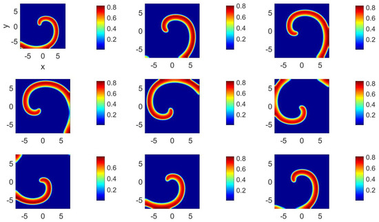
Figure 1. (Color online) $u(t,x,y)$ at (from left to right and top to bottom) $t=50$, 55, 60, 65, 70, 75, 80, 85, and 90 for parameter set 1001.

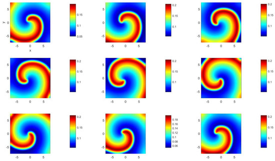
Figure 2. (Color online) $v(t,x,y)$ at (from left to right and top to bottom) $t=50$, 55, 60, 65, 70, 75, 80, 85, and 90 for parameter set 1001.

For set 1002, the results presented in Figure 3 and Figure 4 also correspond to a zero-velocity field, indicating that no spiral wave seems to be present; instead, the spatial distribution of u exhibits very small values for long periods of time, large curvature fronts as illustrated in the third and ninth frames, and very small curvature fronts, as shown in the sixth frame in Figure 3. However, the spatial distribution of v presented in Figure 4 indicates the presence of fronts of larger curvatures than those observed in Figure 3.

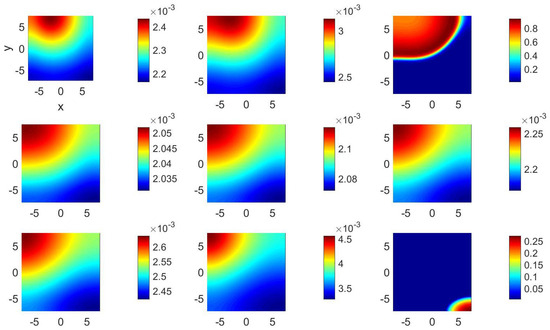
Figure 3. (Color online) $u(t,x,y)$ at (from left to right and top to bottom) $t=50$, 55, 60, 65, 70, 75, 80, 85, and 90 for parameter set 1002.

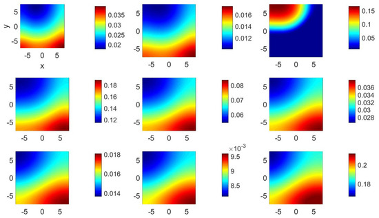
Figure 4. (Color online) $v(t,x,y)$ at (from left to right and top to bottom) $t=50$, 55, 60, 65, 70, 75, 80, 85, and 90 for parameter set 1002.

Although not shown here, similar results to those in Figure 3 and Figure 4 were obtained for set 1003 of Table 1, indicating that $d_{12}$ has a much larger effect on the spiral wave dynamics than $D_{21}$. In fact, as indicated in Table 1, the results for sets 1000 and 1001 have the same periods, which are much smaller than those of sets 1002 and 1003.

Figure 4 also indicates that even though v undergoes large changes, they are smaller than those seen in Figure 3. The reason for this behavior will become clear later on after presenting the time histories of u and v at three fixed locations within the computational domain.

In order to understand in greater detail the dynamics of the solution, the values of u and v at three spatial locations were monitored as functions of time. These points are located at $\left(-{\displaystyle \frac{L}{2}},-{\displaystyle \frac{L}{2}}\right)$, $(0,0)$ and $\left({\displaystyle \frac{L}{2}},{\displaystyle \frac{L}{2}}\right)$, i.e., they are located along the main diagonal of the computational square domain, at the center and halfway between the center of the domain, and at the lower-left and upper-right corners, respectively.

Figure 5 shows the time traces at the three monitoring locations for sets 1000, 1001, 1002, and 1003 of Table 1, clearly indicating that the periods of u and v for sets 1000 and 1001 are nearly identical, indicating that $D_{12}$ does not play an important role in the wave dynamics. By way of contrast, Figure 5 also shows that the results corresponding to sets 1002 and 1003 are nearly identical, but have larger periods than those of the results of sets 1000 and 1001.

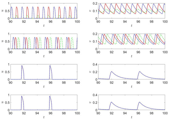
Figure 5. (Color online) $u(t,x,y)$ (left) and $v(t,x,y)$ (right) at $(x,y)=\left(-{\displaystyle \frac{L}{2}},-{\displaystyle \frac{L}{2}}\right)$ (continuous line, red), $(0,0)$ (dashed line, green) and $\left({\displaystyle \frac{L}{2}},{\displaystyle \frac{L}{2}}\right)$ (dashed-dotted line, blue) for parameter set 1000 (first row), 1001 (second row), 1002 (third row), and 1003 (third row).

A detailed view of the first two rows in Figure 5 also indicates that the magnitude of v at $\left({\displaystyle \frac{L}{2}},{\displaystyle \frac{L}{2}}\right)$ is much smaller compared to the other two monitoring locations. Figure 5 also shows that the largest amplitudes of u and v for sets 1000 and 1001 are smaller and larger, respectively, than those for sets 1002 and 1004.

4.2. The Effects of Anisotropy in the Presence of Velocity Field

Figure 6 shows the time histories of both u and v for sets 1011, 2008, 2009, and 2010 in Table 1 and Table 2. These sets correspond to a counter-rotating vortex field characterized by $\omega =2.5$, $R=1$ and various values of $D_{12}$ and $d_{12}$. The results obtained for $(D_{12},d_{12})=(0.05,0)$ have been found to differ very little from those corresponding to $(D_{12},d_{12})=(0,0)$, i.e., the isotropic case, and quite a lot from those corresponding to $(D_{12},d_{12})=(0,0.05)$ which, in turn, were found to differ very little from those for $(D_{12},d_{12})=(0.05,0.05)$, once again indicating that $D_{12}$ does not play an important role in the wave dynamics.

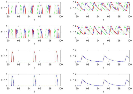
Figure 6. (Color online) $u(t,x,y)$ (left) and $v(t,x,y)$ (right) at $(x,y)=\left(-{\displaystyle \frac{L}{2}},-{\displaystyle \frac{L}{2}}\right)$ (continuous line, red), $(0,0)$ (dashed line, green) and $\left({\displaystyle \frac{L}{2}},{\displaystyle \frac{L}{2}}\right)$ (dashed-dotted line, blue) for parameter set 1011 (first row), 2008 (second row), 2009 (third row) and 2010 (third row).

Consistent with previously discussed results for $\omega =0$, the results presented in Figure 6 show that the maximum values of u and v for $(D_{12},d_{12})=(0,0)$ and (0.05, 0) are smaller and larger, respectively, than those for $(D_{12},d_{12})=(0,0.05)$ and (0.05, 0.05), and the period of the latter is larger than that of the former. Figure 6 also shows that the peak values of u and v are nearly of the same magnitudes for $(D_{12},d_{12})=(0,0)$ and (0, 0.05) (cf. compare with Figure 5).

Similar trends to those corresponding to the two last rows in Figure 6 have also been found in the results corresponding to sets 1002, 1006, 1009; 1003, 1007, 1009; 1002, 5005, 2025; 2009, 2013, 2021, 2025; 1008, 4005, 5005; etc. However, some surprising results were obtained for sets 1023 and 2025 and are illustrated in Figure 7 and Figure 8.

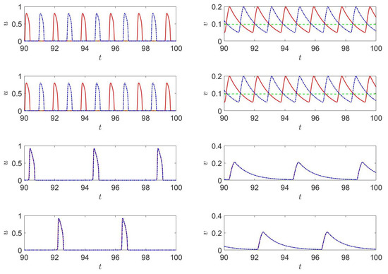
Figure 7. (Color online) $u(t,x,y)$ (left) and $v(t,x,y)$ (right) at $(x,y)=\left(-{\displaystyle \frac{L}{2}},-{\displaystyle \frac{L}{2}}\right)$ (continuous line, red), $(0,0)$ (dashed line, green) and $\left({\displaystyle \frac{L}{2}},{\displaystyle \frac{L}{2}}\right)$ (dashed-dotted line, blue) for parameter set 1023 (first row), 2020 (second row), 2021 (third row) and 2022 (third row).

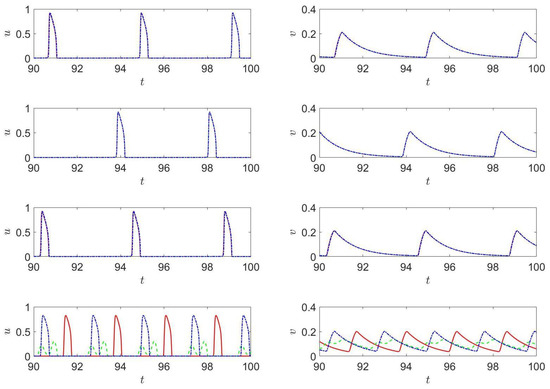
Figure 8. (Color online) $u(t,x,y)$ (left) and $v(t,x,y)$ (right) at $(x,y)=\left(-{\displaystyle \frac{L}{2}},-{\displaystyle \frac{L}{2}}\right)$ (continuous line, red), $(0,0)$ (dashed line, green) and $\left({\displaystyle \frac{L}{2}},{\displaystyle \frac{L}{2}}\right)$ (dashed-dotted line, blue) for parameter set 2009 (first row), 2013 (second row), 2021 (third row), and 2025 (third row).

Figure 7 shows similar trends to those observed previously in Figure 5 and Figure 6. However, a major difference is seen for sets 1023 and 2025, i.e., u and v reach very small values at $\left({\displaystyle \frac{L}{2}},{\displaystyle \frac{L}{2}}\right)$, but their values at the other two monitoring locations differ very little from each other and exhibit a saw tooth pattern. This indicates that no front passes through the location $\left({\displaystyle \frac{L}{2}},{\displaystyle \frac{L}{2}}\right)$.

The time histories at the three monitoring locations for sets 2009, 2013, and 2021 presented in Figure 8 show similar trends to those exhibited in the last two rows in Figure 7; however, those for set 2025, corresponding to a larger and faster clockwise-rotating velocity field, are nearly identical at the monitoring locations $\left(-{\displaystyle \frac{L}{2}},-{\displaystyle \frac{L}{2}}\right)$ and (0,0). On the other hand, the v history profile at $\left({\displaystyle \frac{L}{2}},{\displaystyle \frac{L}{2}}\right)$ is of a smaller magnitude and exhibits two relative maxima. The reason for this behavior will become clear when the two-dimensional distributions of u and v at selected times are presented.

In order to further illustrate the effects that anisotropy may have on two-dimensional systems of second-order hyperbolic, nonlinear advection–reaction–diffusion equations, the two-dimensional distributions of v for sets 1024 and 1026 are presented at selected times in Figure 9 and Figure 10, respectively.

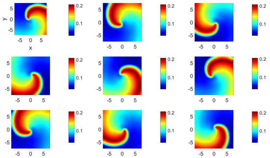
Figure 9. (Color online) $v(t,x,y)$ at (from left to right and top to bottom) $t=50$, 55, 60, 65, 70, 75, 80, 85, and 90 for parameter set 1024.

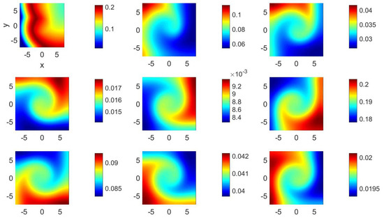
Figure 10. (Color online) $v(t,x,y)$ at (from left to right and top to bottom) $t=50$, 55, 60, 65, 70, 75, 80, 85, and 90 for parameter set 1025.

Figure 9 clearly illustrates the presence of a counter-rotating spiral wave, which is thicker and rotates much more slowly than that exhibited in Figure 2. The reason for this slowdown is that the results in Figure 9 correspond to a clockwise rotating field, which is contrary to the counter-rotating spiral wave, and the vortex diameter is large. No velocity field was used to obtain the results reported in Figure 2.

Although not shown here, analogous results to those in Figure 9 have been obtained for set 1027, corresponding to the same parameters as those of Figure 9 except for $D_{12}=0.1$, thus indicating once again that the anisotropy of the variable u does not play an important role in the qualitative and quantitative characteristics of the solution to Equation (20).

For the parameters in set 1025, the results presented in Figure 10 are quite different from other results presented previously in this manuscript. For example, the first frame in that figure illustrates a small curvature thick front, whereas the remaining eight frames show vortex-like shapes that remind the reader of the engulfment of fluids in, for example, planar mixing layers (cf., e.g., Figures 3 and 9 in Reference [31]).

4.3. The Effects of Relaxation Times on Wave Propagation

The effects of ${\tau }_u$ and ${\tau }_v$ on the solution were found to be small for relaxation times less than 0.05, which, according to the estimates discussed in this paper, correspond to a velocity along the characteristics equal to $\sqrt{20}$ and $\sqrt{12}$ for u and v, respectively. For the domain considered in this study, whose dimensions in the x and y directions are 15, the times required for the propagation from, say, the left to the right boundary range from 3.35 to 4.33. By way of contrast, the characteristic diffusion times for u and v based on L are 56.25 and 93.75, respectively. These times are clearly much larger than those associated with propagation along the characteristic lines. This means that the effects of the relaxation times are expected to be small and, in fact, they have been found to be small, except in a thin initial layer near $t=0$ whose time duration is on the order of the relaxation time consistent with the asymptotic analysis of singularly perturbed wave equations, e.g., [32,33,34].

In order for the characteristic time based on the velocity along the characteristic lines and the diffusion time to be of the same order of magnitude, Equation (19) demands that $\tau =\mathcal{O}\left(L^2\right)$ which, for the domains considered here, implies that $\tau \approx 56.25$, and, for such a large relaxation time, the Taylor series expansion of Equation (5), i.e., Equation (6), is not valid.

5. Conclusions

A time-linearized, three-time-level finite difference method for the numerical solutions of multivariable, multi-dimensional, second-order hyperbolic, advection–reaction–diffusion equations has been presented and applied to analyze the effects of relaxation, convection, and anisotropy on the heat and mass diffusion fluxes in a two-variable, two-dimensional problem. The equations are based on a frame-indifferent constitutive model for the diffusion flux that, for zero relaxation times, reduces to the Fourier law. This model has been formulated for both temperature and species concentrations and can also address the variables of their diffusion fluxes.

It has been shown that the anisotropy of one of the dependent variables plays a very minor role in the numerical solution, whereas the anisotropy of the other variable leads to transitions from spiral waves to fronts of large curvature, and then to fronts of smaller curvature. The solutions corresponding to these fronts have been found to have longer periods than those associated with isotropic diffusion. It has also been found that the concentration peak values of the two dependent variables differ from those obtained for isotropic diffusion.

For small anisotropy in the diffusion tensors and counterclockwise-rotating vortices of small radii, the effect of the velocity field is to stretch and strain the spiral waves, whereas, for clockwise vortices, convection leads to wave compression and deceleration. Similar results to those just described have been found for isotropic diffusion. However, for clockwise-rotating vortices of large diameters in anisotropic media, complex transitions have been observed as the vortex circulation increases. These transitions are characterized by highly distorted spiral waves for small vortex circulations, large curvature fronts for moderate circulations, and wave trapping for large circulations. The wave trapping observed in large-diameter, clockwise-rotating vortical fields exhibits similarities with vortex development and entrainment seen experimentally in non-reactive planar mixing layers.

For large-diameter, counterclockwise-rotating vortices, it has been found that the effects of anisotropy are almost identical at three points located on the main diagonal of the computational square domain employed in the numerical experiments reported here. Only transitions from spiral waves to fronts of large curvatures and then fronts of small curvatures are observed as the vortex circulation increases.

The effects of the relaxation times of the two dependent variables considered in this study are important primarily within an initial layer. This layer’s duration is on the order of the largest relaxation time, where the solution undergoes a rapid transition from the initial conditions to those corresponding to parabolic advection–reaction–diffusion equations, consistent with well-known results of the asymptotic analysis of singularly perturbed, second-order hyperbolic equations. This initial adjustment has been solved accurately in the numerical experiments reported here, where a time step two orders of magnitude smaller than the smallest relaxation time was used, and does not have a cumulative effect in time, so that the long-term behaviors of the equations considered in this paper are identical to those for parabolic advection–reaction–diffusion equations.

For the conditions considered in this study, it has also been shown that relaxation effects may be important for large relaxation times, for which the well-known linear relaxation equation is not valid. Therefore, studies based on such large relaxation times may be of academic interest but may not be relevant to heat and mass transport phenomena, which are usually characterized by small relaxation times, although they may be relevant for the modeling of forest fires, virus infections, the spread of epidemics, chemical reactions, biology, ecology, population dynamics, etc.

References

- Landau, L.D.; Lifshitz, E.M. Fluid Mechanics; Pergamon Press: New York, NY, USA, 1987. [Google Scholar]
- Joseph, D.D.; Preziosi, L. Heat waves. Rev. Mod. Phys. 1989, 61, 41–73. [Google Scholar] [CrossRef]
- Joseph, D.D.; Preziosi, L. Addendum to the paper “Heat waves” [Rev. Mod. Phys. 61, 41 (1989)]. Rev. Mod. Phys. 1990, 62, 375–391. [Google Scholar] [CrossRef]
- Murray, J.D. Mathematical Biology II: Spatial Models and Biomedical Applications; Springer: New York, NY, USA, 2003. [Google Scholar]
- Ritchie, J.S.; Krause, A.L.; Van Gorder, R.A. Turing and wave instabilities in hyperbolic reaction–diffusion systems: The role of second-order time derivatives and cross–diffusion terms on pattern formation. Ann. Phys. 2022, 444, 169033. [Google Scholar] [CrossRef]
- Pourasghar, A.; Chen, Z. Hyperbolic heat conduction and thermoelastic solution of functionally graded CNT reinforced cylindrical panel subjected to heat pulse. Int. J. Solids Struct. 2019, 163, 117–129. [Google Scholar] [CrossRef]
- Rubin, M.A. Hyperbolic heat conduction and the second law. Int. J. Engng Sci. 1992, 30, 1665–1676. [Google Scholar] [CrossRef]
- Christov, C.I. On frame indifferent formulation of the Maxwell–Cattaneo model of finite–speed heat conduction. Mech. Res. Commun. 2009, 36, 481–486. [Google Scholar] [CrossRef]
- Christov, C.I. On the material invariant formulation of Maxwell’s displacement current. Found. Phys. 2006, 36, 1701–1717. [Google Scholar] [CrossRef]
- Truesdell, C. A First Course in Rational Continuum Mechanics; Academic Press: New York, NY, USA, 1977. [Google Scholar]
- Zhmakin, A.I. Non–Fourier Heat Conduction: From Phase-Lag Models to Relativistic and Quantum Transport; Springer Switzerland AG: New York, NY, USA, 2023. [Google Scholar]
- Williams, F.A. Combustion Theory, 2nd ed.; Addison–Wesley Publishing Company: New York, NY, USA, 1985. [Google Scholar]
- Vanag, V.K.; Epstein, I.R. Cross–diffusion and pattern formation in reaction–diffusion systems. Phys. Chem. Chem. Phys. 2009, 11, 897–912. [Google Scholar] [CrossRef]
- Shi, J.; Xie, Z.; Little, K. Cross–diffusion induced instability and stability in reaction–diffusion systems. J. Appl. Anal. Comput. 2010, 24, 95–119. [Google Scholar] [CrossRef]
- Carslaw, H.S.; Jaeger, J.C. Conduction of Heat in Solids; Oxford University Press: New York, NY, USA, 1959. [Google Scholar]
- Bertaglia, G.; Pareschi, L. Hyperbolic models for the spread of epidemics on networks: Kinetic description and numerical methods. ESAIM Math. Model. Numer. Anal. 2021, 55, 381–407. [Google Scholar] [CrossRef]
- Barbera, E.; Currò, C.; Valenti, G. A hyperbolic reaction–diffusion model for the hantavirus infection. Math. Methods Appl. Sci. 2008, 31, 481–499. [Google Scholar] [CrossRef]
- Méndez, V.; Casas–Vázquez, J. Hyperbolic reaction–diffusion model for virus infection. Int. J. Thermodyn. 2008, 11, 35–38. [Google Scholar]
- Méndez, V.; Llebot, J.E. Hyperbolic reaction–diffusion model for a forest fire model. Phys. Rev. E 1997, 56, 35–38. [Google Scholar] [CrossRef]
- Consolo, G.; Curró, C.; Grifó, G.; Valenti, G. Oscillatory periodic pattern dynamics in hyperbolic reaction–advection–diffusion models. Phys. Rev. E 2022, 105, 034206. [Google Scholar] [CrossRef] [PubMed]
- Cho, U.-I.; Eu, B.C. Hyperbolic reaction–diffusion equations and chemical oscillations in the Brussellator. Phys. D 1993, 68, 351–363. [Google Scholar] [CrossRef]
- Al–Ghoul, M.; Eu, B.C. Hyperbolic reaction–diffusion equations and irreversible thermodynamics: Cubic reversible reaction model. Phys. D 1996, 90, 119–153. [Google Scholar] [CrossRef]
- Al–Ghoul, M.; Eu, B.C. Hyperbolic reaction–diffusion equations, patterns, and phase speeds for the Brusselator. J. Phys. Chem. 1996, 100, 18900–18910. [Google Scholar] [CrossRef]
- Zemskov, E.P.; Horsthemke, W. Diffusive instabilities in hyperbolic reaction–diffusion equations. Phys. Rev. E 2016, 93, 032211. [Google Scholar] [CrossRef]
- Ramos, J.I. Numerical methods for nonlinear second-order hyperbolic partial differential equations. I. Time–linearized finite difference methods for 1-D problems. Appl. Math. Comput. 2007, 190, 722–756. [Google Scholar] [CrossRef]
- Greenbaum, A. Iterative Methods for Solving Linear Systems; SIAM: Philadelphia, PA, USA, 1997. [Google Scholar]
- Meurant, G. Computer Solution of Large Linear Systems; North-Holland: Amsterdam, The Netherlands, 1999. [Google Scholar]
- Saad, Y. Iterative Methods for Sparse Linear Systems, 2nd ed.; SIAM: Philadelphia, PA, USA, 2003. [Google Scholar]
- Simoncini, V.; Szyld, D.B. Recent computational developments in Krylov subspace methods for linear systems. Numer. Linear Algebra Appl. 2007, 14, 1–82. [Google Scholar] [CrossRef]
- Ramos, J.I. Propagation of spiral waves in anisotropic media: From waves to stripes. Chaos Solitons Fractals 2001, 12, 1057–1064. [Google Scholar] [CrossRef]
- Bernal, L.P.; Roshko, A. Streamwise vortex structure in plane mixing layers. J. Fluid Mech. 1986, 170, 499–525. [Google Scholar] [CrossRef]
- Kevorkian, J.; Cole, J.D. Perturbation Methods in Applied Mathematics; Springer: New York, NY, USA, 1981. [Google Scholar]
- Kevorkian, J.; Cole, J.D. Multiple Scale and Singular Perturbation Methods; Springer: New York, NY, USA, 1996. [Google Scholar]
- Butuzov, V.F. The angular boundary layer in mixed singularly perturbed problems for hyperbolic equations. Math. USSR Sb. 1997, 33, 403–425. [Google Scholar] [CrossRef]
Disclaimer/Publisher’s Note: The statements, opinions and data contained in all publications are solely those of the individual author(s) and contributor(s) and not of MDPI and/or the editor(s). MDPI and/or the editor(s) disclaim responsibility for any injury to people or property resulting from any ideas, methods, instructions or products referred to in the content. |
© 2024 by the author. Licensee MDPI, Basel, Switzerland. This article is an open access article distributed under the terms and conditions of the Creative Commons Attribution (CC BY) license (https://creativecommons.org/licenses/by/4.0/).