Abstract
Vulnerability mapping of sea-coastal zones is an important element of oil spill response plans, environmental support for offshore projects, and the integrated management of the marine environment. The creation of such maps is a complex scientific problem. In their development, it is necessary to take into account differences in the nature of biotic and abiotic components existing in the cartographic area, dissimilarities in their relative vulnerability and significance, the seasonal variability of ecosystem components, and other factors. The purpose of this paper is to briefly review the main elements of international and Russian methods of mapping the vulnerability of sea-coastal zones to oil spills, and the development problems of such maps, including problems of using rank (ordinal) values, and to note possible solutions. Based on the analysis of key existing international and Russian approaches to vulnerability mapping, it was concluded that almost all methods of map calculations use rank (ordinal) values. However, arithmetic operations cannot be performed with them, as they lead to incorrect results. The paper shortly describes the main problems of mapping the vulnerability of sea-coastal zones to oil (the choice of the map scales and season limits for them, differences in the units of biota abundance, the calculation of relative vulnerability coefficients for the considered biotic components, the summation of the vulnerability of objects of different types, etc.). For some problems, possible solutions are outlined.
1. Introduction
Prospecting, extraction, and maritime transportation of oil require special attention to environmental safety, notably with respect to accidental oil spills in the shelf zones. In this regard, the problem of developing and using sensitivity/vulnerability maps of sea-coastal zones to oil is especially urgent. These maps should be used in the planning of oil spill response (OSR) activities, as well as in the course of these activities [1,2]. Such maps are able to minimize the potential damage from oil spills to natural and man-made environments. Specialists distinguish between two types of maps. Sensitivity maps represent the sensitivity of a shoreline to oil, which is ranked by the environmental sensitivity index (ESI). There is a corresponding well-developed procedure for the creation of such maps; these are widely used outside Russia [1,2,3,4,5]. Vulnerability maps represent the integrated vulnerability of sea areas to oil spills, describing all negative consequences, possible damage to biological resources, social and economic objects, and nature conservation territories, should a spill occur. This paper considers the water areas near the coast (sea-coastal zones), although a similar approach to vulnerability assessment is fully applicable to the water areas that are more remote from the shoreline.
The recommendations of international organizations [1,2] and some other methods [6,7,8], emphasize that in order to minimize oil spill damage, it is necessary to take into account both the vulnerability of sea-coastal zones and the sensitivity of the shoreline by the ESI index. We do not dwell on examples of sea oil spills because there are a lot of reviews focusing on this problem (for example, extensive bibliography [9] and bibliography of accident with oil platform in the Gulf of Mexico [10]). Detailed analysis of important incidents is given in [11,12,13] and many other publications. Spills statistics concerned with tanker accidents are represented in ITOPF material [14].
In this paper we consider only issues of the methodology to construct the maps of water area vulnerability. There is still no consensus on the procedure of vulnerability maps construction. These maps are compiled by different methods in different countries; they are supposed to have some general correct provisions and principles. The best situation is when the sensitivity or vulnerability maps of neighboring countries that have access to the sea are prepared by a single or similar method, and both are used in OSR, including joint operations. It is important for coordinating the actions of these countries’ liquidators in large-scale oil accidents affecting the neighbor states.
It should also be noted that a general methodology for constructing the maps of a marine environment’s vulnerability to oil can be used to make vulnerability maps and assess possible damage to the environment in any offshore project, for any form of anthropogenic impact. A unified methodology can be employed for constructing the maps of marine environment vulnerability to spills of oil and oil products (spills in accidents with tankers, oil platforms, underwater oil pipelines), reservoir water (accidents in shelf drilling) or suspended matter (in dredging and dumping of the ground), and acoustical action (working oil platforms, tubing, freight by large-capacity vessels). With an appropriate common algorithm, differences can only be accounted for in vulnerability coefficients of the considered groups/subgroups/biota species. This general approach is determined by the following: (1) the main base of the natural and man-made environment data for vulnerability mapping is one and the same for different types of exposure; (2) the coefficients of biota vulnerability themselves from different anthropogenic impacts may differ in one of the parameters, e.g., sensitivity and/or potential effect (the details are given below); (3) the algorithm for calculating such maps is virtually the same.
Except for OSR operations, such vulnerability maps are necessary for: (1) conducting preliminary environmental studies in the area of the possible impact of a project (in Russia they are called engineering and environmental surveys), which is required for environmental support and justification of the environmental safety of planned economic activities; (2) assessing the zone of their possible impact during normal operation and in emergency situations; (3) integrated management of marine environments, including the integrated management of coastal zones; (4) planning of environmental monitoring.
In and outside of Russia, there is experience in constructing vulnerability maps [6,7,8,15,16,17,18], but the calculations of water area integrated vulnerabilities are usually based on ordinal values (ranks) and the application of associated arithmetic operations. However, the latter is infeasible with rank values [19,20,21,22]. Otherwise, vulnerability maps constructed on this basis are incorrect. At the same time, refusal to use ordinal values leads to several methodic problems. Therefore, any research in this area—developing a correct methodology for constructing vulnerability maps of water areas—is significant and rather complicated, especially with regard to the total vulnerability of a large number of biological objects in one area. The Appendix provides a brief justification and an example of the fact that using rank values in arithmetic operations, including the calculation of vulnerability maps, leads to incorrect results.
The purpose of this paper is to briefly review the main elements of international and Russian methods of mapping the vulnerability of sea-coastal zones to oil spills, and the development problems of such maps, including problems of using rank (ordinal) values, and to note possible solutions.
2. A Brief Overview of Methods for Constructing Vulnerability Maps
Vulnerability maps for oil are based on different approaches in different countries. The main methods are referred to below. In their consideration, it is more important to pay attention to the correctness of vulnerability maps, their clarity, and comprehensibility for the user, rather than the complexity or simplicity of the methodology. A rigorous approach is also significant.
2.1. The International Organizations—International Marine Organization (IMO), International Petroleum Industry Environmental Conservation Association (IPIECA), International Association of Oil & Gas Producers (IOGP)
These organizations prepared reports [1,2] on the mapping of environmentally vulnerable zones for oil spill response. In this report [2], the terms “sensitivity” and “vulnerability” are not explained, no distinction is made between them, and the term “sensitivity” is used, with very few exceptions. The term “sensitivity” always refers to the effects of marine environment pollution associated with accidental hydrocarbon spills (verbatim: ‘Within this guide, ‘sensitivity’ always relates to the effects of accidental marine pollution involving hydrocarbons’).
Vulnerability maps are a key stage in the preparation of OSR, and an essential tool for liquidators. The map scale is a very important element for the methodology and the end product. The nature and volume of necessary initial data, the volume of cartographic materials, and the possibility of liquidators to use such maps depend on scale. Let us consider the report of 2012 [2]. The maps are prepared by the working group during the preparation of OSR plans. There are three levels of spills—from Tier 1 (a small spill) to Tier 3 (a large-scale spill)—and three map scales corresponding to them: 1:10,000–1:25,000 (object-related), 1:25,000–1:100,000 (tactical), and 1:200,000–1:1,000,000 (strategic). At different stages of the OSR, they use one or more sets of maps, depending on the level of the spill.
Tactical maps are developed in the first instance and are fundamental for operations managers and field coordinators. They show: (1) the type of the shoreline by the ESI index; (2) sensitive ecosystems, habitats, biological species, and key natural resources; data on their concentration can be expressed in a simplified manner (presence/absence in ranks/points from 1 (no information) to 5 (high abundance of species)); (3) social and economic objects: ports, aquaculture, etc.; (4) logistic and other important resources for OSR; (5) potential sources of oil spills.
Strategic maps are prepared based on tactical maps; they are intended for the OSR headquarter management team. They represent: (1) the most sensitive types of the coastline, for example, only ESI 8 index as high and ESI 9–10 indices as very high; and the other types (low sensitivity) may not be shown; (2) the ranked sensitivity of ecosystems and native resources (a five-point scale from very low to very high); (3) the ranked sensitivity of socio-economic resources in a manner similar to the previous parameter. To determine the rank sensitivity of the site, there is a recommended matrix (Figure 1). It is recommended that an assessment of the site’s sensitivity be undertaken in terms of the diversity of sensitive species (the abscissa axis) and the sensitivity of those species (the ordinate axis). A similar scheme can be used to rank socio-economic sites and nature conservation areas.
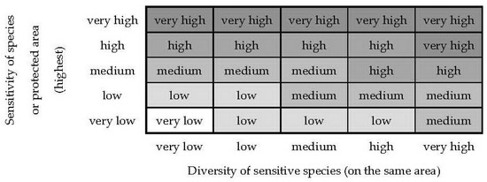
Figure 1.
The matrix for ranking the sensitivity of a site with a wide range of biological species and other objects [2]. This simple matrix can be used to establish a sensitivity ranking for an area where a diverse range of sensitive species is present, by comparing the sensitivity of the species/protected area with the diversity of species in that area [2] (reproduced with permission from IPIECA, 2018).
This is an approach based on rank assessment values. It doesn’t involve performing arithmetic operations with the values of sensitivity and species diversity, although neither of the two matrix scales is a metric ratio scale (the rational zero and unit of measurement are not defined).
In our opinion, the most important point here is that this approach does not take into account the abundance (biomass or number per unit area) of individual groups/subgroups/species of biota. Abundance also largely defines the impact of oil on the site. Thus, the greater the biota abundance within a site, the more (with other conditions remaining the same) negative the consequences (possible damage) of an oil spill for it, and the more priority should be given to such a site in terms of oil spill protection. The presented matrix and the approach described in the report do not allow for this fact, since sensitivity and vulnerability are not distinguished. It was already noted that the report [2] uses only the concept of “sensitivity”, which is not defined in this document. This concept can be interpreted as the presence of one or another reaction to the effect of a negative factor on one or another organism. To our mind, it is more optimal to talk of area vulnerability as of the total negative effects from oil spills, taking into account not only biota sensitivity, but also a number of other characteristics, including the abundance of biota in the area and its recoverability rate after a spill. For example, we may compare two zones. With a “medium” level of sensitivity of one or two mass species (“very low” diversity), the sensitivity of the first zone will be “medium” (Figure 1). Also with a “medium” sensitivity of species, but their “high” diversity and “low” total abundance, the sensitivity of the second zone will be “high”. At the same time, the vulnerability (overall negative consequences) of the first zone may be greater than that of the second zone, just because of the greater abundance of species. In addition, the restorability rate of certain species is not taken into account at all. With other conditions remaining the same, the consequences (vulnerability of the zone) are more serious, based on the recovery rate of the species after a spill.
Operational maps are optional maps for liquidators and field coordinators; they are developed for the most sensitive areas and high-risk areas. These maps show detailed information about logistics and operational resources for OSR, data on the protection of specific vulnerable resources and areas, as well as information on the protection system for a specific object and details of planned OSR operations.
2.2. The Model of OSR Mapping in Norway (Modellen for Miljoprioriteringer—MOB)
The Norwegian Climate and Pollution Agency (Statens forurensningstilsyn) issued the document “Emergency Pollution Prevention—Model for prioritizing environmental resources for an acute oil spill in the coastal zone” [6]. This model is still in force. The authorities of coastal territories prepared maps according to this method. In case of an oil pollution threat to the sea areas adjacent to the territory, these maps must be used to coordinate the administration experts in oil spill response operations. The method is based on the classification of natural resources (biological, geographical, physical, chemical) and human activity objects according to four factors: natural occurrence, compensability, conservational value, and general oil vulnerability, which are estimated as ranks/points (Table 1).

Table 1.
Estimation of the factor in the MOB model [6] (reproduced with permission from Miljødirektoratet, Norway, 2018).
For all objects, vulnerability tables are shown on a point (or rank) scale: for biological objects (groups/subgroups/species of birds, marine mammals, fish)—in the integer range between 0 and 3; for the types of shores and objects of nature management—in the range between 0 and 2. After multiplying all the factors (P = VI × VII × VIII × VIV) for each object, they obtain one of the five priority protection categories: A (P = 36), B (P = 18 or 24), C (P = 9 or 12), D (P = 4 or 6 or 8), E (P ≤ 3). These categories Psx (where s is the index of the calendar season, x is the reference number) are plotted on maps along with the boundaries of the corresponding objects’ distribution or location. The maps are supplemented with a table containing a detailed description of each resource. The map scale is 1:100,000–1:200,000 (actually, they are tactical maps).
The maps take into account all of the most important biological, social, and economic resources, as well as the sensitivity of the coastline. All important information on resources is collected in a single format, which can be used both for OSR and for other environmental purposes. Two or more priority categories marked on the different areas does not change the protection priority of area where they may overlap. In addition, maps are developed for the whole year (although it is recommended that they be constructed for distinct seasons in exceptional cases). This, as well as the description of the resource priorities provided in the tables, may hinder the liquidators or coordinators in making a decision or undertaking action because they need to address both to the maps and to tables with resource descriptions in order to decide about the presence or absence of the corresponding resource in the area. Also, the use of rank values in calculating the priority category (P) of individual objects is not correct (see Appendix A).
2.3. The Method to Construct Environmental Vulnerability Maps in the Economic Zone of the Netherlands
The method was developed by the National Institute for Coastal and Marine Management (RIKZ, The Hague) [15]. Its experts prepared seasonal maps for the vulnerability of the Dutch Exclusive Economic Zone to various pollutants, including oil. The basis for their development is biota seasonal abundance in each map cell (5 × 5 km) and the vulnerability of biota to toxic agents. Ecosystem components should be represented by the major groups of biota (benthic and pelagic invertebrates, fish, birds, mammals), and related habitats. The method takes into account (1) biota species and their habitats for all vertical zones: near the seabed (zoo benthos), those moving freely in the water column (pelagic species), those found near the sea surface (birds) and the coast (phytobenthos); (2) the habit complex of these biota species (flight, swimming, diving, hunting) and the features of typical habitats (seabed, water column, sea surface, shore), in order to assess the potential impact of the pollutant on them.
The behavior of pollutants in the environment is divided, according to the Standard European Behavior Classification (SEBC code, Bonn Agreement), into five main types: gases, evaporators, floaters, dissolvers, sinkers. The mechanisms of their actions are based on the European criteria of persistence, bioaccumulation, and toxicity. Vulnerability is determined by three values: the potential effect (E) of the pollutant on the ecosystem component, its sensitivity (S) to the active factor, and the recoverability (R) of the component after exposure cessation. The values E, S, and R are calculated from a number of parameters; the final vulnerability (V) is calculated by the formula: V = (E × S)/R. All the parameters for the calculation of these three values are estimated expertly on the basis of points/ranks, mainly in the integer range between 0 and 10. Seasonality is also considered. To construct biota distribution maps, initial abundance (spec/km2, kg/m2) is normalized and reduced to non-dimension parameters. The scale of these maps is 1:100,000.
The negative point in this approach is that all the parameters used for calculations and mapping are assessed as ranks (if regarded as points, these are not “values” for the metric scale). Most likely, the maps provide strategic, small-scale reference points, especially since the objects of possible protection from oil spills and other pollutants within the area 25 km2 are represented on the map as one element. The mapping model takes into account the biota and its habitats, as well as various socio-economic objects. However, there is no mention of how these two components are “added” when calculating the final area vulnerability. In a practical implementation, this method turned out to be difficult and is not used currently. Nevertheless, the very approach to the calculation of biological objects vulnerability proposed in this work seems important. In our view, it is advisable to use it in any methodology for constructing vulnerability maps.
2.4. The Method to Calculate Environmental Vulnerability to Oil Spills and Other Chemicals in the Baltic Sea (the BRISK Project)
In 2009–2012, the Baltic countries carried out the project “Sub-regional risk of spill of oil and hazardous substances in the Baltic Sea” (BRISK) [16]. It was a response to the concerns about the growth of accidents and environmental damage in the sea because of a significant increase in shipping, particularly oil tanker transportation. The project involved all the countries of the Baltic Sea, including Russia.
An integral part of the project is mapping the vulnerability of the Baltic Sea to oil and other hazardous chemical substances. Construction of vulnerability maps is a small part of the whole project; they serve as a foundation for calculating possible environmental damage in various scenarios of pollutant spills (Risk of damage = Probability of oil spills × Vulnerability). To reduce the risk in an area, possessing information on its vulnerability is essential.
The methodology for constructing vulnerability maps is very briefly described in the document [16]. It covers 17 different objects (natural and socio-economic resources), each with a distribution map. The maps (positions or areas without biota abundance quantities) are based on expert evaluation, taking into account the available information. The expert ecological seasonal vulnerability of each object is ranked as an integer from 0 to 4 (1—low, 4—very high). For each calendar season, all 17 maps are integrated into one map by summation of the distribution of corresponding objects, multiplied by their vulnerability coefficients. The vulnerability values on the integrated maps change in the range, approximately, between 0 and 40. This range is divided into 5 sub-ranges for better perception, from low to high vulnerability (or from dark green to red on the maps). The map scale is 1:500,000 (strategic maps).
The map resources were selected after project discussions. The vulnerability ranking is based on knowledge about the physical and biological characteristics of different ecosystems, organisms, or socio-economic resources, and their response to oil. Experts considered the behavior of oil, its potential impact on organisms and their habitats, and the recoverability of respective components after exposure; abiotic components were also taken into account. Given the incorrectness of the vulnerability calculation (because it is based on arithmetical operations with ranks), the assessments of pollutant spill damage risk are incorrect as well.
2.5. The Methodology to Construct Integrated Environmental Vulnerability Maps by CJSC “Ecoproject” and World Wildlife Fund (WWF) Russia
The leading author of the development in CJSC “Ecoproject” is Doctor of Biological Sciences V. Pogrebov [7]. The WWF methodology is the result of specialists’ teamwork under the guidance of WWF Russia [8]. This methodology is completely based on the approach of CJSC “Ecoproject”. The company has developed and improved it, but has not changed its principles. Starting from the 1990s, the works of V. Pogrebov and his team in creating vulnerability maps was practically unique in Russia. They greatly contributed to the development of this sphere in the country, and initiated broad discussions on the topic of working groups; their seminars were organized by WWF Russia.
According to the approach that gave a start to the Ecoproject method, the potential environmental vulnerability of a water area in a particular season is determined by the abundance of organism groups that inhabit that area and their varied vulnerability to oil [7]. The algorithm is as follows. Specialists determine the limits of seasons, define objects for evaluation (all environmental groups, from phytoplankton to birds), and make maps of abundance distribution for them (rank distribution based on points). The coefficients of biota vulnerability (in terms of sensitivity and recoverability) are evaluated expertly as integer points, in the range from 1 to 5; the potential impact of oil on the biota groups is not considered, but there are individual vulnerability coefficients for dispersed oil and oil films. In addition to biota, the method takes into account zones of special significance, e.g., water protection areas, vulnerable habitats, etc., but they do not constitute a separate group, and the vulnerability coefficients for them are not given. Initial maps are converted to geographic information system (GIS) data, represented in the form of layers on a regular grid, the cell size of which is based on the minimum size of the map contours.
Another step in the calculation of vulnerability maps is the spatial “summation” of all initial maps developed for the ranked ecological groups’ abundance, taking into account their vulnerability coefficients as ordinal values. The obtained results are seasonal maps of vulnerability to oil (and/or other types of exposure). The integrated vulnerability is represented on maps by five color gradations—from green (low vulnerability) to red (high vulnerability), but the algorithm for dividing by subranges is not described. The maps have one specified scale. The maps developed according to procedure [7] are used in many Russian OSR plans and in offshore project materials. This process is based entirely on the use of ranks (non-metric points), which is not correct. Using cells instead of polygons for data representation distorts biota distribution and the positions of objects, and can hinder the orientation of liquidators during OSR.
WWF Russia’s method [8] recommends the use of polygonal distribution of sensitive objects, but it also involves rank evaluation of species abundance. Two groups of objects are evaluated separately: biotic components, or important ecosystem components, and vulnerable socio-economic objects, or areas of priority protection. The map scale depends on a particular purpose and the level of oil spill: there are plans (1:10,000–1:25,000), large-scale (1:25,000–1:100,000), and small- and medium-scale (1:100,000–1:1,000,000) maps. For vulnerability factors in this method, it is proposed to use a table, which is more detailed than in [7], but also the range of the ranks is the same, from 1 to 5. The method calculations use polygonal shapefiles, but all sample vulnerability maps are presented in [8] with a division of the calculation area into individual cells, like in [7]. The coastline sensitivity maps should also support the ESI requirements.
Thus, given that these methods are based on the use of ranks, it is possible to speak of incorrectness of the maps developed with them.
2.6. The Methodology of Murmansk Marine Biological Institute (MMBI) for Constructing Vulnerability Maps
The methodology developed at MMBI [17,18] was initially based on the methods outlined in [7,8], but was fundamentally different from them in some aspects. The methods were similar in the following points: (1) all initial values for calculation (biota abundance distribution, biota vulnerability coefficients) were estimated in most cases as rank values (in the ranges 1–5 and/or 1–10); (2) the integrated vulnerability of a site was the total abundance of biota groups/subgroups multiplied by the corresponding vulnerability coefficients; (3) final vulnerability maps had the form of individual cells, although the calculation applied polygonal distribution.
However, this method differs from the Ecoproject /WWF Russia procedure in some significant points. Firstly, there were calculations of both relative and absolute integrated vulnerability [17]. The relative integrated vulnerability of the map area was presented as several (three-five) subranges of the total range of the area’s integrated vulnerability in a given season. This range is different for each season. The absolute integrated vulnerability in a particular season is represented as 3–5 subranges of the total range of the area’s integrated vulnerability for the whole year; the range of vulnerability is single for different seasons. Secondly, the selection of seasons was based on the limits of the periods of the year, i.e., the periods when the distribution densities of biota groups/subgroups are approximately constant [18]. With this approach, the number of seasons can differ from the number of conventional calendar periods. It should be noted that in the first version of the methodology to calculate the vulnerability maps for the eastern part of the Barents Sea [17], seasons were defined before the construction of maps for the biota groups’ abundance distribution. Nevertheless, for large marine areas, it is only possible to use an approach that takes into account the seasonal variability of biota for various parts of the map area. Thirdly, it is the use of metric, dimensionless units of biota abundance (groups/subgroups distribution density), rather than rank values in subsequent specific calculations, that became possible due to normalizing the initial distributions to the average annual abundance of groups in the mapping area [18,23]. However, even partial use of rank values (relative vulnerability coefficients) also makes the methodology incorrect.
A comparison of the main elements of the vulnerability mapping method of sea-coastal zones to oil is represented in Table 2. It is possible to draw an overall conclusion from the comparison and short analysis of the considered methods: all these methods are not quite correct because they are based on the use of ordinal values (ranks) in different stages of calculations; however, this is not acceptable, and leads to incorrect maps. We recommend against the use of ranks in vulnerability maps calculation entirely.
Table 2.
Main elements comparison of vulnerability mapping method of sea-coastal zones to oil.
We propose a new, more correct procedure of vulnerability mapping (briefly presented in [24,25], which is completely based on the use of only metric values. It also assumes a fundamentally different approach to assessing the specific vulnerability of biota groups with different interactions with water (see below Section 3.4, Section 3.5 and Section 3.6). This direction requires further research, since the “metric” methods still have unresolved questions and difficulties. Some of them are described below in Section 3.
3. Main Problems in the Development of Vulnerability Maps
We believe that in order to construct sea-coastal vulnerability maps correctly, one should consider vulnerable objects and their specific (relative) vulnerability. For the correct assessment of coastal marine vulnerability to oil, it is necessary to have the following information: (1) the quantitative characteristics of seasonal spatial distribution of biota ecological groups/subgroups/species (their abundance) on all sites of the evaluated area; (2) the specific vulnerability of these biota groups/subgroups/species to oil; (3) the position of the considered abiotic (socio-economic, nature-conservative) objects in the evaluated area, which are not directly related to the biota abundance; (4) the degree of their significance for human beings. In fact, the latter parameter is the evaluation of coefficients of abiotic objects’ significance, an analogue of biota specific vulnerability. All values must be appropriate for the metric ratio scale.
The development of vulnerability mapping procedures has different problems. These are the main ones, taking into consideration the absence of ranks and points.
3.1. Selection of Vulnerability Mapping Scale
It is recommended developing maps on different scales only in one method [2]. Our proposals for map scales are as follows (all scale values are tentative and require detailed discussion). Strategic small-scale maps (1:500,000 and less) give a general representation of the most vulnerable areas. For such maps (covering quite large areas of the sea), it is difficult to correctly identify the seasons, for which the maps are designed (see below). But they are important to OSR senior managers for general strategic planning, especially for large-scale spills. Tactical maps (1:100,000–1:250,000) should probably be prepared for all sea-coastal areas; they are the most numerous vulnerability maps for marine and coastal zones. Object-related maps (1:10,000–1:50,000) must be developed for the most significant marine and sea-coastal areas.
Some questions remain unanswered: what is shown on each of the vulnerability maps of different scales, what the strategic, tactical, and object-related maps have in common, and what their fundamental differences are. The work [2] gives comprehensive recommendations in this respect, and the content of information on maps with different scales is fundamentally dissimilar. We believe that vulnerability maps should be on different scales for cartographic areas. The difference between them should be specified by a generalization in transfer from large-scale to small-scale maps. In any case, this suggestion and recommendations on scales stated in report [2] should be discussed in detail.
3.2. The List of Objects for Evaluation
This is a debatable issue, especially if the development of maps involves specialists working in different fields. It is important to avoid inclusion into this list all or almost all the biota groups inhabiting the cartographic area; only the dominant, essential, and Red Book species should be considered. It is also necessary to take into account socio-economic objects and nature conservation areas. At this stage, the issue should be generally solved using methods which are in line with the recommendations given in the report of international organizations [2].
3.3. Adjustment of Limits for Seasons
It is important to decide about periods—will the map be created for the entire year, for each month, or for certain seasons (climatic, calendar, etc.)? The authors of [17] show that for large areas, e.g., for the whole eastern (Russian) part of the Barents Sea, there can be several proposed variants of such periods, based on different criteria. We believe that the most important criterion for the selection of seasons is the stability of the distribution density of vulnerable objects, primarily biological ones. While preparing the initial data, it is reasonable to start from the periods of the year within which the initial distribution (abundance) of the evaluated biota and the position of abiotic objects remain relatively constant. The seasons for mapping should be chosen with the help of these data on stability [18]. If you construct a series of vulnerability maps of a long-stretching coastal water area for a single season and deal with great variability in many parameters (there is an example of the Barents Sea coast of the Kola Peninsula), you will inevitably face discrepancies between the maps of neighboring sites of the cartographic area. The reason is differences in the time limits of the seasons for the western and eastern parts of the coastal regions. This issue also still requires discussion and solution.
3.4. The Units of Biota Abundance
Usually units of biota abundance are different—spec/km2, kg/m2, g/m3, etc. Integrated map construction requires summarizing the vulnerabilities of individual biota groups (abundance of groups/subgroups/species multiplied by corresponding specific vulnerability). This cannot be done if biota distribution values have different units of measurement. That is why biota abundance must be in the same units as those that have been proposed in [15] for map calculations using cells instead of polygons. Another possible option is a transition to dimensionless units via normalizing the abundance of groups/subgroups/species to the average annual abundance of the corresponding group in the mapping area [23,24,25]. The following is a proposed procedure.
Determine the list of vulnerable components of the ecosystem: important biotic components (IBC), especially significant social-economic objects (ESO), and protected areas (PA). The required information on all these objects, such as results of expeditions, published works, and expert estimates, is assumed to have been collected for the area mapped.
Demarcate seasonal boundaries for this area. When boundaries of the seasons do not coincide with different biotic components (and probably for occurring ESOs), the final number and boundaries of seasons for maps of integral vulnerability are determined by boundaries of corresponding seasons of all biotic groups/subgroups/species and abiotic components that are taken into account.
Make seasonal maps of the distribution of ecosystem components for each adopted scale: IBC density (, s is the season index, g is the biota group index), locations of ESOs and PAs ( and , where e and f are the indices of the corresponding abiotic objects).
Maps of distributing are constructed in the units that are accepted for biotic groups (benthos—g/m2; birds—item/km2).
Normalize seasonal maps (Equation (1)) of distribution of each gth biotic component () to the annual average abundance of the corresponding group within the mapped area (the superscript y indicates that a year is the period under consideration):
This procedure enables us to use identical units of measurement for densities of biota [23]: all biotic components that are taken into account are represented in the units of the share of the annual average abundance of the corresponding group in the mapped region per unit area: (kg/m2)/kg = 1/m2; (item/km2)/item = 1/km2 → 1/m2.
Construct ESO maps, polygons of ( = 1 for ESOs, the remaining water area is 0) and PA maps, polygons of ( = 1 for PAs; the remaining water area is 0).
The normalization of the distribution density of biotic groups/subgroups/species to the annual average abundance () of the corresponding groups makes it possible to represent all biotic components under study in identical units of measurement (shares of annual average abundance of the group within the mapped region per unit area).
Such an approach, like in the previous case, can lead to discrepancies between the maps of neighboring areas, because the maps for each of them are normalized, taking into account the abundance of biota groups/subgroups/species specific for each area. This issue is not finally resolved on this stage.
3.5. Coefficients of Biota (Relative) Vulnerability
Expert evaluation of vulnerability coefficients or the parameters (sensitivity, recoverability, the potential exposure to oil) required for calculating the coefficients of biota specific vulnerability to oil can easily be made in integer ranks or points [6,7,8,15,16,17,18]. The refusal to use rank values leads to a new problem. The indicated parameters are quite difficult to quantify, for both dominant environmental groups and well-studied individual species. Vulnerability coefficients (V) may be calculated as described (in simplified view) in [15]: V = (E × S)/R. Considerable research has been devoted to sensitivity assessments of major biological groups/subgroups/species to oil (evaluation of the values LC50 and/or LL50). The works were carried out both at the end of the last century (e.g., [27,28] and many others) and in recent years, when new methodological approaches were used (e.g., [29,30,31,32] and others). On this basis, it is possible to make quite a realistic estimation of the necessary metric values of S for most biota groups/subgroups/species. The values of S for the remaining objects will be chosen by expert evaluation, but also on the metric ratio scale. The coefficients of potential exposure (E, percentage) and recovery (R, years) are probably easier to manage, because the information about them is extensive and easily available, and the methodological problems are few. Priority protection coefficients for abiotic components should also be presented as metric values on the basis of their social and economic importance.
The choice of a certain scale of units for biota sensitivity (S) is an additional problem. It is possible to distinguish at least 4 habitats: pelagic (fish, plankton), bottom (fish, benthos), littoral (zoobenthos, macrophytobenthos, birds), and sea surface (birds), although this segmentation is quite nominal. Birds, mostly contacting with the water surface, are exposed to oil film (including exposure on littoral areas), but not to oil dissolved or dispersed in water. Fish and plankton are exposed to oil dispersed only in the water column. Thus, the sensitivities of fish/plankton and birds have different scales and cannot be fully compared. A possible solution to this problem is also briefly presented in [24,25].
Vulnerability coefficients for IBSs () should be calculated, and coefficients of priority protection for ESOs () and PAs () expertly evaluated. All values are given in the metric scale (the use of points and ranks is excluded).
For IBCs, the coefficients of are estimated by three parameters (Equation (2)):
where is expressed in years, is in percent, and is in units of values of oil concentrations in the water, or the thickness of an oil film on the water, that are maximum permissible for biota of the components that are taken into account; subscript b denotes the ratio of these parameters to the biota.
Initially, LC50 (the lethal concentration of oil in the water) or LL50 (the lethal load of oil) is taken as the sensitivity of the biota (parameter ) inhabiting the water column [27,28,29,30,31,32]; is normalized to the maximum permissible concentration of oil in the water, MPC: = /MPC.
The thickness of an oil film that causes 50% death of biota (conventionally = LT50) is taken as the sensitivity of biota that mostly contacts the water surface, i.e., an oil film. Then LT50 is normalized to the maximum permissible thickness (MPT) of an oil film that does not produce a considerable effect on these biotic groups: = /MPT.
The values of coefficients of priority protection are expertly selected with respect to the ecological, economical, and/or other importance of objects for humans or the ecosystem of the region. In this case, the ratios between coefficients / and (ei, ej, and fi, fj are the indices of ESO and PA objects) should reflect the ratio of importance between the corresponding objects that is the closest to reality, rather than the “ratios” of rank (ordinal) values.
The normalization of the values of to the maximum permissible concentrations, or the maximum permissible thickness, removes the dependence of this parameter (sensitivity) from that it is related to the water column or to its surface; is expressed in identical units of measurement for all biotic groups/subgroups/species.
This approach also requires more detailed separate consideration, and more precise determination of LC50 (LL50) and LT50 values, including the issues of littoral and benthic communities.
3.6. Summation of Vulnerability for Objects of Different Nature
In constructing vulnerability maps, it is necessary to take into account not only the vulnerability of biota, but also the vulnerability (significance) of abiotic components. Their summation is inevitable, regardless of possible overlapping of biota distribution areas and socio-economic zones/nature conservation areas. We propose the following as a solution to this problem.
Maps of vulnerability for IBCs and maps of priority protection for ESOs and PAs (in fact, maps of ESO and PA vulnerability) based on the data obtained for each season and each scale adopted are constructed as follows.
- For IBCs: = and normalize the values obtained for each season:
- —to max per season for maps of relative vulnerability = / per season);
- —to max per year for maps of absolute vulnerability = / per year).
- For ESOs: = and normalize the values obtained for each season:
- —to max per season for maps of relative vulnerability = /( per season);
- —to max per year for maps of absolute vulnerability = /( per year).
- For PAs, perform the same procedure as for ESOs.
- Make seasonal maps of integral vulnerability of the region:
- —for maps of relative vulnerability ;
- —for maps of absolute vulnerability ,
where Kb,c,d are coefficients (estimated expertly) that determine the contribution of IBCs, ESOs, and PAs to the integral vulnerability.
The range of values of vulnerability is divided into three subranges for each season (they are given ranks (1, 2, 3): each season has its own range of values of min ÷ max . Here, ranks can be used, since this is the final stage of mapping and no further mathematical operations are performed with the data, except for comparisons of the obtained values shown in the maps.
The range of values of vulnerability is also divided into three subranges (they are given ranks (1, 2, 3): each season has a common range of values of min ÷ max .
The segments with different ranks are shown in different colors: green (rank 1 is the minimum values of ), yellow (rank 2), and red (rank 3 is the maximum values of ).
In addition, here vulnerability maps for each season are developed for two different ranges. Relative vulnerability maps: for each season there is a unique range of vulnerability (min ÷ max for specific season). Absolute vulnerability maps—for all seasons of the year, there is one, common range of vulnerability (min ÷ max for the year).
3.7. Representation of Water Area Total Vulnerability (the Problem of Classification)
The maps should contain the areas of the highest and lowest vulnerability for planning operations of OSR or for the waters and shores cleaning. Representation of these zones on maps is a result of vulnerability calculations (performed with the use of GIS programs). It partly depends on the choice of the method for classifying the final range of integrated vulnerability to subranges (the methods of equal intervals, natural breaks, etc.). This choice also affects the overall picture of site vulnerabilities. The classification of subranges may possibly be such that the maps of sea-coastal zones would reflect, along the shoreline, areas with a low, medium, and high vulnerability in an approximately equal manner (proportions). This direction also requires further research.
There are other problems of mapping the vulnerability of sea-coastal areas to oil: whether it is necessary to create separate vulnerability maps for oil with various densities, how to take into account the hydrological situation in the area (for example, the density jump layer), the ice conditions, etc.
4. Conclusions
Vulnerability maps of sea-coastal zones are important elements of oil spill response plans, environmental support for offshore projects, preparation of the Environmental Impact Assessment, and integrated marine environmental management. The compilation of such maps is a complex scientific problem. When developing them, it is necessary to take into account the presence of different biotic and abiotic components in the cartographic area’s ecosystem, differences in their specific vulnerability, seasonal variability of components, spills of different types of oil, and other factors.
Coastal sensitivity maps and water vulnerability maps have been developed and are being used in many countries. The brief analysis of several existing international and Russian methods for the mapping of sea-coastal vulnerability to oil allows us to draw the following conclusions. The majority of the reviewed methods are based on arithmetic operations with rank values. For all the simplicity of the approach, it is not acceptable, and leads to incorrect vulnerability maps. Using such maps, in turn, results in erroneous spill liquidators’ actions in terms of the minimization of damage to the environment from both oil spills and the operations aimed to eliminate them. It is necessary to reject the use of rank estimates of parameters if the latter are used in arithmetic operations during calculation of vulnerability maps.
The article also briefly describes the main problems of constructing the maps of sea-coastal vulnerability to oil. For some problems, the main solutions are outlined. We suppose that, despite the complexity of these problems, acceptable and rational solutions exist. The necessary conditions are initial rigor of the approach to development of mapping algorithm. There is a need to consider existing mathematical rules and restrictions, processes of oil spreading in water, regularities of biota distribution and behavior, and oil impact on it. Simplifications and assumptions should be done on the later stages of calculations considering the complexity of all processes and the necessity of clearly showing the vulnerable zones on the maps. Only this will allow us to create correct and comprehensible maps of sea coast vulnerabilities to oil for OSR plans. This direction requires further investigation and the joint efforts of researchers, experts, and liquidators of spills from different countries.
Author Contributions
A.S. and A.K. analyzed presented methods and wrote the paper. All authors read and approved the final manuscript.
Funding
This research was funded by FASO number in state assignment of MMBI KSC RAS 01 2013 66838.
Acknowledgments
This paper is based on the results of scientific research performed for the state assignment of MMBI KSC RAS “Evaluation of vulnerability and ecological monitoring of Arctic ecosystems during offshore development” (State Registration No. 01 2013 66838).
Conflicts of Interest
The authors declare no conflict of interest.
Appendix A
Appendix A.1. Rank Values in Arithmetic Operations
In the development of vulnerability maps, many algorithms for their calculation assume execution of arithmetic operations. Then there is a question: is it feasible to use the variables presented on ordinal (rank) scales in such calculations? This question is discussed in detail in several publications [19,20,21,22]. The sequence of numerical characteristics of a value can be denoted by any method as they increase, for example, by a series of natural numbers. These are ranks. But they are not numerical (metric) values. They are mere markers that reflect the order of objects. They do not reflect the correlation of values. Using ranks (points) is permitted if they are arithmetized. Then all the resulting dimensions on the linear ordinary scale, which have no numeric character, take the form of numerical information [21]. But this operation is usually not performed in constructing vulnerability maps.
Let us give an example of arithmetic operations when the values X and Y are represented on the metric scale with a rational zero (ratio scale) and on the rank (order) scale. Let us normalize the metric values Xm and Ym and represent them as ranks (Xr and Yr)—please, see the left part of the example table. The obtained products of the ranks Xr × Yr do not reflect the sequence of products of these values Xm × Ym on the metric scale (the right part of the example Table A1).
Table A1.
Example of arithmetic operations—on the metric and on the rank (order) scales.
Table A1.
Example of arithmetic operations—on the metric and on the rank (order) scales.
| Initial Values X and Y on the Metric (m) and Rank (r) Scales | The Product X × Y of Metric (Xm × Ym) and Rank (Xr × Yr) Values | |||||||
|---|---|---|---|---|---|---|---|---|
| X | Xm | Xr | Y | Ym | Yr | X × Y | Xm × Ym | Xr × Yr |
| A | 50 | 1 | P | 60 | 5 | A × P | 50 × 60 = 3000 | 1 × 5 = 5 |
| B | 60 | 2 | Q | 40 | 4 | C × Q | 70 × 40 = 2800 | 3 × 4 = 12 |
| C | 70 | 3 | R | 30 | 3 | A × Q | 50 × 40 = 2000 | 1 × 4 = 4 |
| D | 110 | 4 | S | 10 | 2 | E × S | 120 × 10 = 1200 | 5 × 2 = 10 |
| E | 120 | 5 | T | 4 | 1 | B × S | 60 × 10 = 600 | 2 × 2 = 4 |
If actual quantities are not known and replaced with ranks, performing operations with them as operations with metric numbers leads to incorrect results. In arithmetic operations, including calculation of sea-coastal vulnerability maps to oil, it is unacceptable to use any values if all or even some of them (biota density distribution, biota vulnerability, etc.) are ranks or points (in case points are not presented on the metric ratio scale). This approach may lead to incorrect results (to incorrect vulnerability maps). The latter means that in reality the most vulnerable areas can be marked as areas having an average or even low vulnerability and vice versa. The use of such vulnerability maps in OSR will not minimize the damage from oil spills and reduce the OSR operations efficacy.
References
- International Maritime Organization (IMO); International Petroleum Industry Environmental Conservation Association (IPIECA). Sensitivity Mapping for Oil Spill Response; IPIECA: London, UK, 1994; Volume 1. [Google Scholar]
- International Petroleum Industry Environmental Conservation Association (IPIECA); International Maritime Organization (IMO); International Association of Oil & Gas Producers (OGP). Sensitivity Mapping for Oil Spill Response; IPIECA: London, UK, 2012. [Google Scholar]
- Gundlach, E.R.; Hayes, M.O. Vulnerability of coastal environments to oil spill impacts. Mar. Technol. Soc. 1978, 12, 18–27. [Google Scholar]
- Petersen, J.; Michel, J.; Zengel, S.; White, M.; Lord, C.; Plank, C. Environmental Sensitivity Index Guidelines; Ver. 3.0. Technical Memorandum NOS OR&R 11; NOAA Ocean Service: Seattle, WA, USA, 2002.
- Introduction to Environmental Sensitivity Index Maps. NOAA, 2008; 56p. Available online: http://response.restoration.noaa.gov/sites/default/files/ESI_Training_Manual.pdf (accessed on 18 September 2018).
- Statens Forurensningstilsyn (SFT). Beredskap Mot Akutt Forurensning—Modell for Prioritering av Miljøressurser ved Akutte Oljeutslipp Langs Kysten; TA-nummer 1765/2000; SFT: Oslo, Norway, 2004; ISBN 82-7655-401-6. (In Norwegian)
- Pogrebov, V.B. Integral assessment of the environmental sensitivity of the biological resources of the coastal zone to anthropogenic influences. In Basic Concepts of Modern Coastal Using; RSHU: St. Petersburg, Russia, 2010; Volume 2, pp. 43–85. (In Russian) [Google Scholar]
- World Wildlife Fund (WWF). Methodological Approaches to Ecologically Sensitive Areas and Areas of Priority Protection Map Development and Coastline of the Russian Federation to Oil Spills; Vladivostok: Moscow/Murmansk/St. Petersburg, Russia, 2012. (In Russian) [Google Scholar]
- Fiolek, A.; Pikula, L.; Voss, B. Resources on Oil Spills, Response, and Restoration: A Selected Bibliography. Library and Information Services Division, Current References 2010-2, June 2010, revised December 2011. Available online: ftp://ftp.library.noaa.gov/noaa_documents.lib/NESDIS/NODC/LISD/Central_Library/current_references/current_references_2010_2.pdf (accessed on 18 September 2018).
- Belter, C. Deepwater Horizon: A Preliminary Bibliography of Published Research and Expert Commentary. NOAA Central Library Current References Series No. 2011-01; First Issued: February 2011; Last Updated: 13 May 2014. Available online: https://repository.library.noaa.gov/view/noaa/10854 (accessed on 18 September 2018).
- Albaigés, J.; Bernabeu, A.; Castanedo, S.; Jiménez, N.; Morales-Caselles, C.; Puente, A.; Viñas, L. The Prestige Oil Spill. In Handbook of Oil Spill Science and Technology; Fingas, M., Ed.; John Wiley & Sons, Inc.: Hoboken, NJ, USA, 2015; pp. 513–545. ISBN 978-0-470-45551-7. [Google Scholar]
- Sweet, S.T.; Kennicutt, M.C., II; Klein, A.G. The Grounding of the Bahía Paraíso, Arthur Harbor, Antarctica: Distribution and Fate of Oil Spill Related Hydrocarbons. In Handbook of Oil Spill Science and Technology; Fingas, M., Ed.; John Wiley & Sons, Inc.: Hoboken, NJ, USA, 2015; pp. 547–556. ISBN 978-0-470-45551-7. [Google Scholar]
- Siddiqi, H.A.; Munshi, A.B. Tasman Spirit Oil Spill at Karachi Coast, Pakistan. In Handbook of Oil Spill Science and Technology; Fingas, M., Ed.; John Wiley & Sons, Inc.: Hoboken, NJ, USA, 2015; pp. 557–573. ISBN 978-0-470-45551-7. [Google Scholar]
- The International Tanker Owners Pollution Federation Limited (ITOPF). Oil Tanker Spill Statistics 2017. London, 2018. Available online: http://www.itopf.org/fileadmin/data/Photos/Statistics/Oil_Spill_Stats_2017_web.pdf (accessed on 18 September 2018).
- Offringa, H.R.; Låhr, J. An Integrated Approach to Map Ecologically Vulnerabilities in Marine Waters in the Netherlands (V-Maps); RIKZ working document RIKZ 2007-xxx; Ministry of Transport, Public Works and Water Management, Rijkswaterstaat, National Institute for Marine and Coastal Management: Hague, The Netherlands, 2007.
- Sub-Regional Risk of Spill of Oil and Hazardous Substances in the Baltic Sea (BRISK). Environmental Vulnerability; Doc. No. 3.1.3.3, Ver. 1; Admiral Danish Fleet HQ, National Operations, Maritime Environment: Copenhagen, Denmark, 2012.
- Shavykin, A.A.; Ilyn, G.V. An Assessment of the Integral Vulnerability of the Barents Sea from Oil Contamination; MMBI KSC RAS: Murmansk, Russia, 2010. (In Russian) [Google Scholar]
- Shavykin, A.A. A method for constructing maps of vulnerability of coastal and marine areas from oil. Example maps for the Kola Bay. Bull. Kola Sci. Centre RAS 2015, 2, 113–123. (In Russian) [Google Scholar]
- Sachs, L. Statistische Auswertungsmethoden (Methods of Statistical Analysis), 3rd revised and expanded ed.; Springer: Berlin/Heidelberg, Germany, 1972. [Google Scholar]
- Glantz, S.A. Primer of Biostatistics, 7th ed.; The McGraw-Hill Companies: New York, NY, USA, 2012; ISBN 978-0071781503. [Google Scholar]
- Khovanov, N.V. Analysis and Synthesis of Indicators in Information Deficit; SPbU: St. Petersburg, Russia, 1996. (In Russian) [Google Scholar]
- Orlov, A.I. Organizational-Economic Modeling: In 3 Parts. Part 2: Expert Evaluation; Bauman MSTU: Moscow, Russia, 2011. (In Russian) [Google Scholar]
- Shavykin, A.A.; Kalinka, O.P.; Vashchenko, P.S.; Karnatov, A.N. Method of Vulnerability Mapping of Sea-Coastal Zones to Oil, Oil Products and Other Chemical Substances. RF. Patent 2613572, 17 March 2017. (In Russian). [Google Scholar]
- Shavykin, A.A.; Matishov, G.G.; Karnatov, A.N. A Procedure for mapping vulnerability of sea-coastal zones to oil. Dokl. Earth Sci. 2017, 475, 907–910. [Google Scholar] [CrossRef]
- Shavykin, A.A.; Karnatov, A.N. Method of Vulnerability Mapping of Sea-Coastal Zones to Oil, Oil Products and Other Chemical Substances Based on Calculations with Metric Values. RF. Patent 2648005, 21 March 2018. [Google Scholar]
- International Maritime Organization (IMO); International Petroleum Industry Environmental Conservation Association (IPIECA). Sensitivity Mapping for Oil Spill Response; IPIECA: London, UK, 2010. [Google Scholar]
- Rice, S.D.; Moles, D.A.; Karinen, J.F.; Kern, S.; CarIs, M.G.; Brodersen, C.C.; Gharrett, J.A.M.M. Effects of Petroleum Hydrocarbons on Alaskan Aquatic Organisms: A Comprehensive Review of All Oil-Effects Research on Alaskan Fish and Invertebrates Conducted by Theauke Bay Laboratory, 1970–81; NOAA: Silver Spring, MD, USA, 1984.
- Markarian, R.K.; Nicolette, J.P.; Barber, T.R.; Giese, L.H. A Critical Review of Toxicity Values and an Evaluation of the Persistence of Petroleum Products for Use in Natural Resource Damage Assessments; API Publication Number 4594; American Petroleum Institute: Washington, DC, USA, 1995. [Google Scholar]
- French-McCay, D.P. Development and application of an oil toxicity and exposure model, OILTOXEX. Environ. Toxicol. Chem. 2002, 21, 2080–2094. [Google Scholar] [CrossRef] [PubMed]
- Environmental Impacts of Arctic Oil Spills and Arctic Spill Response Technologies. Literature Review and Recommendations December 2014. Arctic Oil Spill Response Technology Joint Industry Programme. Available online: http://neba.arcticresponsetechnology.org/assets/files/Environmental%20Impacts%20of%20Arctic%20Oil%20Spills%20-%20report.pdf (accessed on 18 September 2018).
- Gardiner, W.W.; Word, J.Q.; Word, J.D.; Perkins, R.A.; McFarlin, K.M.; Hester, B.W.; Word, L.S.; Ray, C.M. The acute toxicity of chemically and physically dispersed crude oil to key Arctic species under Arctic conditions during the open water season. Environ. Toxicol. Chem. 2013, 32, 2284–2300. [Google Scholar] [CrossRef] [PubMed]
- Dupuis, A.; Ucan-Marin, F. A Literature Review on the Aquatic Toxicology of Petroleum Oil: An overview of Oil Properties and Effects to Aquatic Biota; Canadian Science Advisory Secretariat: Vancouver, BC, USA, 2015.
© 2018 by the authors. Licensee MDPI, Basel, Switzerland. This article is an open access article distributed under the terms and conditions of the Creative Commons Attribution (CC BY) license (http://creativecommons.org/licenses/by/4.0/).