Tidal Datums with Spatially Varying Uncertainty in North-East Gulf of Mexico for VDatum Application

Abstract

We conducted a VDatum-spatially varying uncertainty study for the North-East Gulf of Mexico. The newly developed tide model incorporated the latest available National Ocean Service (NOS) bathymetry survey data and National Geodetic Survey (NGS) shoreline data, and the datum products reflected the updated tidal datum data from the Center for Operational Oceanographic Products and Services (CO-OPS). A gridding technique based on the wavelength of long waves in the deep ocean was applied to improve model efficiency. In this study, we highlight the creation of the tidal datum products and associated spatially varying uncertainty, which was developed by blending the model results, observations, and measurement errors together using a spatially varying uncertainty method based on a variational approach. The study found that model errors, measurement errors, and lack of observations can contribute to large uncertainty in the tidal datum products. The need for high quality bathymetry data in coastal areas is essential for reducing model error. As for the large uncertainty due to lack of observations or large measurement error, this can be improved by placement of new observations with high precision. Compared to a single uncertainty value, the spatially varying uncertainty provides more accurate representation of the uncertainty for the tidal datum products in VDatum. The uncertainty results will be used to help with decision-making on placement of new tide gauges to further reduce the uncertainty in the VDatum products.

1. Introduction

Merging bathymetric and topographic datasets across the land–water interface to create seamless data in the coastal zone is an essential requirement for the protection, management and study of coastal zone processes [1]. The need for accurate data in the coastal zone is increasing and many federal agencies, universities, state and local governments, and other organizations have been collecting high-resolution bathymetry, topography, and shoreline data [2]. Traditionally, data collections by different groups have been operated independently, resulting in data being referenced to different vertical datums. For example, the U.S. Geological Survey (USGS) National Elevation Dataset topographic data are referenced to ellipsoid-based and/or orthometric datums [3], while National Oceanic and Atmospheric Administration (NOAA) National Ocean Service (NOS)’s bathymetry survey and shoreline data are referenced to tidal datums [4]. A pre-requisite for the integration process is to properly reference all such data to a common vertical datum.

To address this requirement, a number of countries in the world are in the process of developing/updating national vertical transformation projects/tools, such as VDatum in the U.S. [5], Vertical Offshore Reference Frames (VORF) in the U.K. [6], BATHYLLI in France [7], etc. [8] These vertical transformation tools utilize tide stations observations and hydrodynamic modeling to evaluate the difference between tidal datums and the geoid [8].

The VDatum vertical datum transformation software is an outcome of the national VDatum project in the U.S., a joint effort of the tri-office VDatum team of NOAA’s Office of Coast Survey (OCS), National Geodetic Survey (NGS), and Center for Operational Oceanographic Products and Services (CO-OPS). The primary purpose is to transform geospatial data vertically between three major classes of vertical datums: tidal, orthometric, and ellipsoid-based datums. At present, VDatum includes 36 different vertical datums. The goal is to have complete coverage of U.S. coastal waters from the landward (i.e., navigable) reaches of estuaries and charted embayments out to 75 nmi offshore [9].

Since its pilot project in Tampa Bay in 2001 [10], VDatum has been created for the continental U.S., Puerto Rico, and the U.S. Virgin Islands. VDatum applications are in development for new areas in Alaska and are also being updated for previous regions to reduce uncertainty. Since the release of VDatum, many applications have benefited from it, including storm surge simulations, tsunami prediction, sea level rise studies [2], ecosystem modeling, and coastal zone management. VDatum also enhances the capabilities of technologies such as kinematic Global Positioning System (K-GPS) for vertical referencing of hydrographic survey depths, use of topographic and bathymetric LiDAR for determining mean lower low water (MLLW) and mean high water (MHW) shorelines, and development of digital elevation models (DEMs).

In this study we focus on tidal datums caused by astronomical tides for VDatum software. VDatum includes a class of seven tidal datums: mean higher high water (MHHW), MHW, mean low water (MLW), MLLW, mean tide level (MTL), diurnal tide level (DTL), and mean sea level (MSL). CO-OPS’ coastal water level stations have been providing these tidal datums data, which are derived from time series of water level data at 6 min intervals. For CO-OPS’ long term control stations, the full 19 year epoch period are used for the computation of the datums [11]. For example, MSL is computed as the arithmetic mean of hourly water observations over the National Tidal Datum Epoch (NTDE), which presently is the 1983–2001 NTDE. All other shorter period subordinate gauges rely on simultaneous comparisons between their data and the epoch control station. The differences between these two stations are applied to the control station datum to acquire a 19 years’ equivalent at the subordinate stations. This helps to mute out the short period meteorological and oceanographic effects which are expected to be experienced by both the control and the subordinate stations.

In general, tidal datum fields vary over horizontal space. Tidal datum data at stations are referenced to measured local water levels and should not be extended into areas having differing oceanographic characteristics. To resolve the spatially varying nature of the tidal datums in between observation locations, hydrodynamic models and spatial interpolation techniques have been employed for each VDatum application that simulate the tidal propagation characteristics in the region of interest. In order to merge all of the individual VDatum applications together to form a continuous national VDatum product, a consistent methodology for computing the tidal datums has been adopted for all region-specific VDatum applications [9]. The approach consists of the following four major steps [2,9]:

(1)

First use the bathymetric and coastline data to develop a grid to be used by the hydrodynamic model.

(2)

Next calibrate a hydrodynamic model to best simulate the observed tidal datum characteristics for the region.

(3)

Then correct the model-data errors using a spatial interpolation technique.

(4)

Finally provide the corrected modeled datums (i.e., datum products) on a structured grid of points to be used by the VDatum software.

Following the above methodology, 38 region-specific VDatum applications have been developed for U.S. coastal regions, among which three of them cover the Gulf of Mexico coast [12,13,14].

For the applications developed prior to 2016, the model-data corrections were made using the Tidal Constituent and Residual Interpolation (TCARI) tool developed by Hess et al. [15,16]. TCARI is a first-order deterministic spatial interpolation tool based on solution of Laplace’s equation. The errors between the model results and the CO-OPS station data are interpolated throughout the domain to create an error field for each of the tidal datums. The error field is then used to correct the model results to create a datum field that matches the station data at those locations [17]. The TCARI approach produces a single-value uncertainty estimate in the tidal datums for each model region [18].

To provide a more accurate representation of the uncertainty in each model region, Shi and Myers developed a new statistical interpolation method, namely the spatially varying uncertainty (SVU) method, for VDatum applications in 2016 [19]. It was derived from the variational principle to calculate the corrected tidal datums by blending the model results, observations, and measurement errors together. They show that the new interpolation approach not only reduces the bias and errors, but also produces a spatially varying uncertainty. The uncertainty results can also provide important guidance for decision-making on placement of new tide gauges to further reduce the uncertainty in the VDatum products. This spatially varying uncertainty method has become the new standard for use for developing VDatum applications since then.

Here we apply Shi and Myers’ method to study spatially varying uncertainty for the north-east Gulf of Mexico (NEGOF) VDatum region (Figure 1). This is part of an effort to update the three VDatum regions in the Gulf of Mexico in the next few years. The SVU study for the Texas VDatum has been completed nearly at the same time and will be published in a separate paper. The Gulf of Mexico coasts have been impacted frequently and severely by past hurricanes, resulting in changes to the coastline and nearshore bathymetry [20]. This can induce uncertainty in the tidal datums in the area. The SVU helps to identify locations where new gauges would be beneficial in reducing uncertainty in VDatum. Once new data is collected, it will then be merged with the model to do a new VDatum update for this region. The same process will be used as we update other VDatum regions as well.

The north-east Gulf of Mexico VDatum region is indicated as the red box in Figure 1. It extends from Mobile Bay, Alabama, in the west to Cape San Blas, Florida, in the east. The region is featured with six bays and relatively flat coastline at the open coast. The bathymetry slope is gentle form shoreline to 40 m water depth and then drops quickly to more than 2000 m deep. The tidal pattern in the region is dominated by diurnal tides [21]. The first version of the tidal model for the region was developed by Dhingra et al. in 2008 [12]. We refer it as the 2008 tidal model in this paper. Since then, new observations on tidal datums and bathymetry survey data have become available. Given the amount of new data, we have redeveloped the tide model to reflect the new information and coverage as best possible.

The rest of this article is organized as follows: Section 2 briefly describes the method; Section 3 presents the data, grid development, and model setup for the new tide model; Section 4 discusses the modeling results, including datum validation, associated spatially varying uncertainty, applications, and lessons learned; summary and conclusion are provided in Section 5.

2. Method

The hydrodynamic model used for this study is the two-dimensional, depth-integrated version of the Advanced Circulation (ADCIRC) model [22,23]. It utilizes the fully non-linear shallow water equations with hydrostatic pressure and Boussinesq approximations. It solves the continuity and the non-conservative momentum equations for free surface elevation and the depth-averaged velocity components. The equations are discretized: horizontally in space using the finite element method with three-node linear triangles; and in time using the finite difference method, the implicit Crank–Nicolson approximation with second order accuracy. The non-linear terms are evaluated explicitly. The ADCIRC code allows a variety of users specified input parameters. Here we used the fully non-linear form of the equations, which includes non-linear bottom friction, finite amplitude, and convection terms. The ADCIRC model has been parallelized using domain decomposition, a conjugate gradient solver, and Message Passing Interface (MPI) based message passing. This parallel version of the code was compiled and run on NOAA’s Jet high performance computing system in Boulder, Colorado. The ADCIRC model has been used in previous VDatum areas [12,13,14], taking advantage of highly flexible, irregularly spaced grids. Numerous studies have shown this model to be robust throughout the Eastern North Atlantic and Gulf of Mexico regions [24,25], and the West Coast [26].

The modeled time series of water surface elevation outputs from the ADCIRC model at each node are then used to tabulate the higher-high, lower-high, higher-low, and lower-low waters, from which tidal datums could be computed. The method for extracting the highs and lows is based on the approach used by CO-OPS [21], which is for analysis of water level measurements at tide stations. The original code is in the C language in the CO-OPS Data Processing and Analysis System (DPAS). The modeled water surface elevation is in general less noisy comparing to the measurements at tide stations. For VDatum, the new Fortran program levels.f (or lv8j.f) was written to duplicate the CO-OPS methodology [9,27]. The program is based on examination of the original C language computer program and related texts, and on discussions with various members of CO-OPS [9]. Seven tidal datums (MHHW, MHW, MSL, MTL, DTL, MLW, and MLLW) are computed based on the highs and lows [21]. The analysis is repeated for time series of water surface elevation at every node in the ADCIRC mesh. We refer to the model datums obtained here as the original model datums (e.g., before correction), to distinguish from the final datum products (after correction with observations). The original model datums are compared to the observations to evaluate the model error.

The next step is to apply the spatially varying method in [19] to the original model datums. The method defines the cost function of the tidal datum field f as:

$$J\left(f\right)=\frac{1}{2}{\left(f-f_m\right)}^T{P}^{-1}\left(f-f_m\right)+\frac{1}{2}{\left(f_0-Hf\right)}^T{\left(W^{-\frac{1}{2}}\right)}^T{R}^{-1}{W}^{-\frac{1}{2}}\left(f_0-Hf\right)$$

(1)

where f is a size (n × 1) vector of the discrete tidal datum product to be determined, f_m is the n × 1 modeled tidal datum field, f₀ is the m × 1 observed tidal datums vector at stations, n is the total node number, m is the total number of tide stations, H is the m × n interpolation matrix projecting the modeled field to the observed data locations, P is the n × n modeled error covariance matrix, R is the m × m observed error covariance matrix, and W is a m × m diagonal weight matrix that adjusts how much the final product f deviated from the uncertainty of the observed values at the station locations. Both the observed tidal datums and error standard deviations are provided by CO-OPS [28]. The weight matrix W is used to control how close the analysis field f is to the observations at the station locations. The constraint that the VDatum technical team adopted for statistical interpolation is that the discrepancy between the analysis field and the observations at all tide stations should be equal to or less than 1 cm or the CO-OPS’ error value, whichever is less. The weight matrix W will be determined through iteration following this predetermined constraint.

By minimizing the cost function J(f) in Equation (1), we obtain the tidal datum product f:

$$f=\underset{f\in {\Re }^n}{\arg \min }J(f)$$

(2)

The uncertainty of f then can be estimated as the posterior error covariance matrix Pa:

$$P_a=Var(f)=(I-GH)P{(I-GH)}^T+GR{G}^T$$

(3)

where $G=P{H}^T{\left[W^{1/2}R{\left(W^{1/2}\right)}^T+HP{H}^T\right]}^{-1}$ is the gain matrix and I is the identity matrix [19]. The datum products f and the spatially varying uncertainty Pa computed from Equations (2) and (3) will be used by the VDatum software.

The spatially varying method produces f and Pa on the same triangular grid as the ADCIRC model. Yet the VDatum software requires regularly spaced grids called “marine grids” that contain the datum information at the water nodes and null information at the land nodes [9]. Digitized coastline data are used to determine which points in this marine grid are water and which are land. Points located within water, or within a distance of approximately one-half a marine grid element size of water, are set to water. The f and Pa based on ADCIRC model grid are then populated in to the marine grids.

The final tidal datum products as represented on the VDatum marine grids must be checked in several ways, including (1) a validation test at station locations, (2) a continuity test at common boundaries, (3) an overlapping test, and (4) a polygon test [9]. For the validation test, the marine grid files are checked against observations to confirm that the datums approximately match at the tide stations. The error at each station should be no greater than 1 or 2 cm. When there are adjacent tidal datum grids, there must be a check for continuity of values across the common boundaries (e.g., continuity test). In some regions, the tidal marine grids can actually overlap, resulting in ambiguity in the selection of the correct grid [9]. Therefore, the use of a bounding polygon is necessary. Given a latitude–longitude point in the overlap region, a check is made of whether the point falls within a specific bounding polygon; if so, the marine grid for that region can be used. If not, additional polygons are checked. The overlapping test is to ensure the bounding polygons do not overlap with each other. The polygon test is to check the bounding polygon to ensure it is completely inside the marine grid [9].

Once the tidal datums f and SVU (Pa) in the marine grids pass the above tests, they will be provided to NGS to incorporate into the VDatum software. In the next section, we will show the details in data and grid development.

3. Data and Grid Development

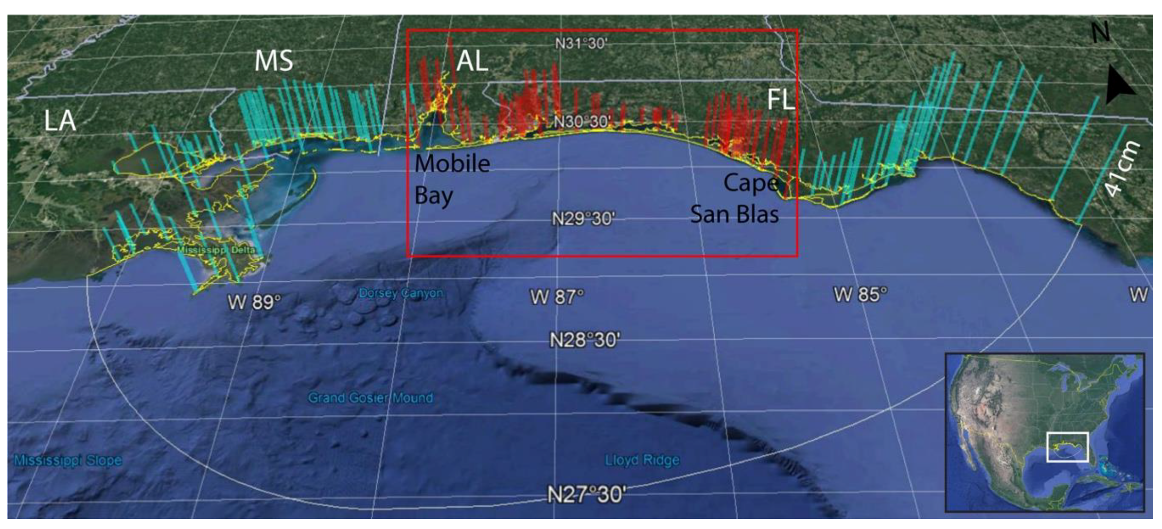
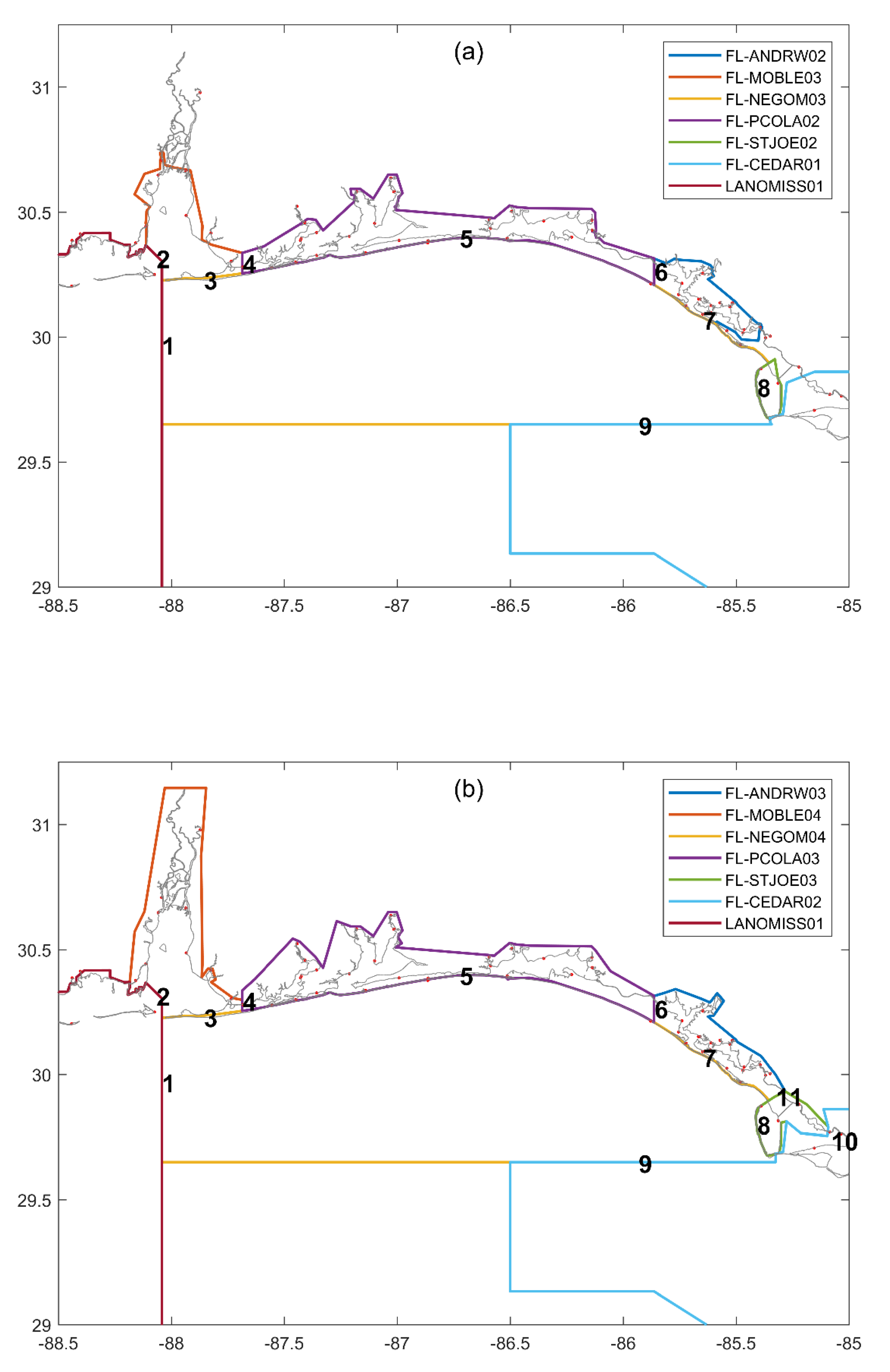
3.1. Study Area and Tidal Datum Data

The VDatum region in this study extends from Mobile Bay, Alabama, in the west to Cape San Blas, Florida, in the east (from −88.0857° E to −85.2811° E). There are 83 NOAA CO-OPS tide stations in the region. Figure 1 shows the station locations and observed MHW datum (the red bars). The height of each bar represents the MHW at the station. As will be discussed in Section 4, stations in the VDatum region show a three-group pattern, which is correlated to their geographical locations. Group 1 stations are located either on the open coast or in less protected bays. This group has the largest tidal datums in the VDatum region, with MHW around 0.18–0.25 m. Group 2 includes the six stations inside Perdido Bay, with MHW around 0.12 m. The third group has the 8 stations inside the Choctawahatchee Bay, with the smallest MHW around 0.08 m. The tidal pattern in the VDatum region is dominated by diurnal tides.

To reduce the boundary effect, we expanded the model domain boundary away from the center of the VDatum region. The domain was extended approximately 5/6 of the width of the VDatum coverage region both to the east and to the west (Figure 1). This introduced 99 additional NOAA tide stations in the computational domain, which are plotted as the cyan bars in Figure 1. The stations located near the east land boundary in Florida have the largest tidal datum in the domain, with MHW around 0.50 m. The tidal pattern in the area is dominated by mixed tides. The tidal datums at the stations to the west are similar to those of Group 1 in the VDatum region except the four stations located inside Lake Pontchartrain, with smaller MHW values around 0.08 m. The tidal pattern in the area is dominated by diurnal tides.

Altogether there are 182 tide stations in the computational domain. The datum measurement error (root mean square error, or RMSE), are available for 144 stations. The average RMSE is 1.7 cm for the 144 stations, with a 2.9 and 3.4 cm maximum within and outside VDatum region, respectively. RMSE are not available for 38 stations due to insufficient data in CO-OPS’ database. Those measurements were mainly from the early 1970s and predated the database (personal communications with CO-OPS’ M. Michalski, 2017). For details on how the RMSE for tidal datums were computed for CO-OPS stations, please see [29].

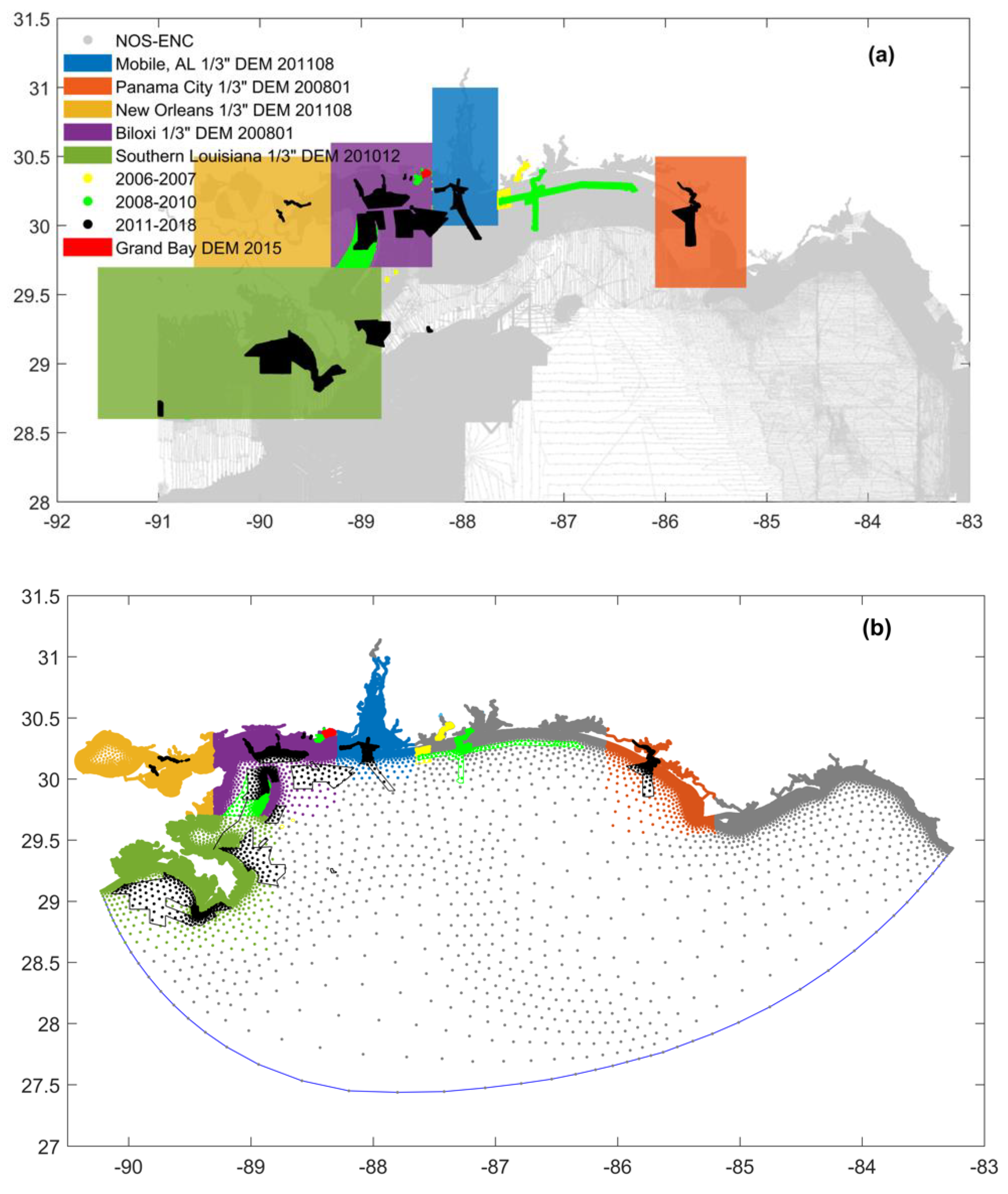
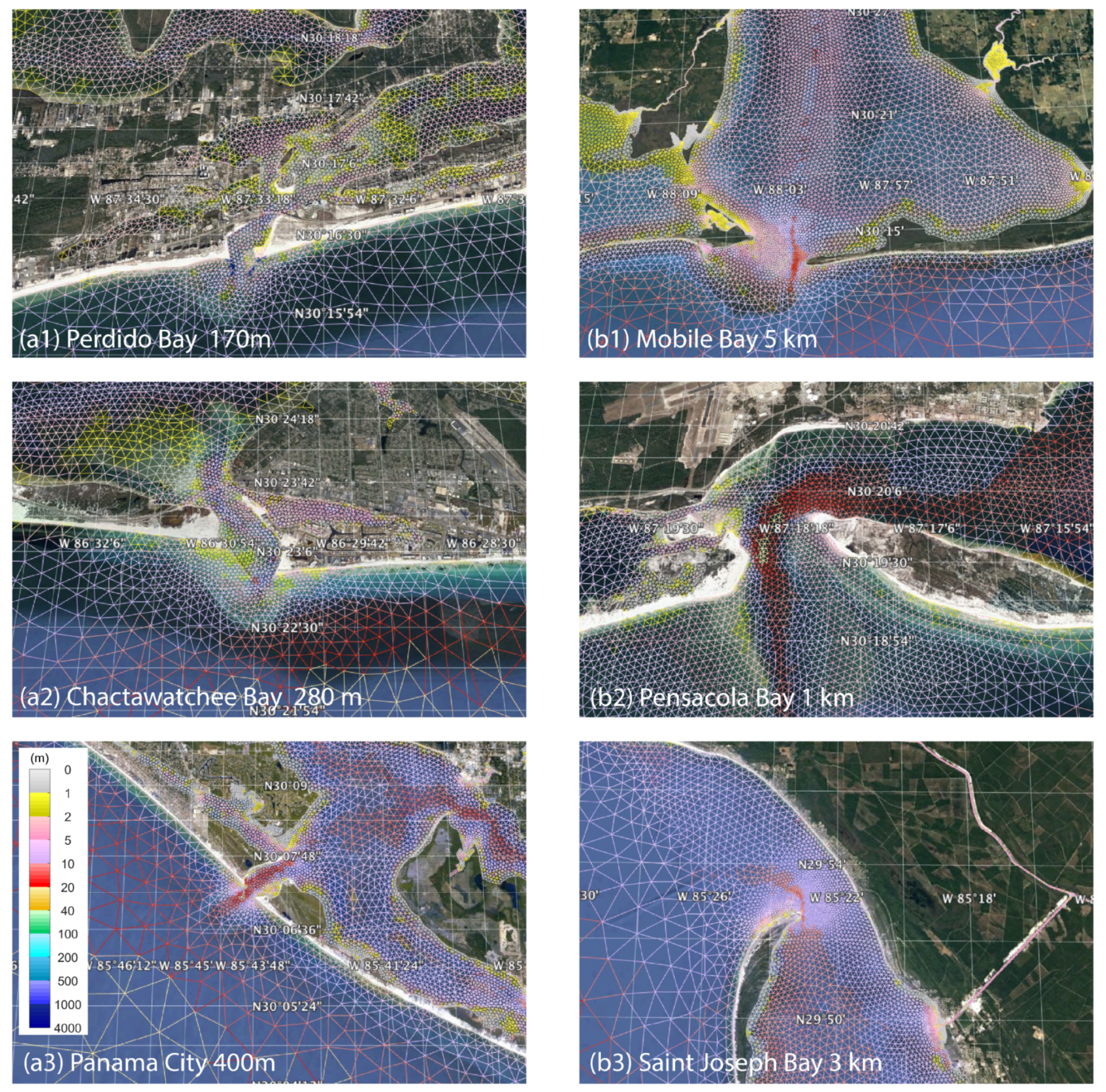
3.2. Shoreline and Bathymetry Data

The MHW coastline was used as the land boundary to create the unstructured grid for the tidal model. It also defines the extent of the VDatum marine grid. The MHW shoreline from NOAA’s Continually Updated Shoreline Product (CUSP) data are considered the most recent and accurate shoreline data available [30]. The horizontal datum is the North American Datum of 1983 (NAD83). The data has scales between 1:1000–1:24,000. Individual national shoreline projects and high-resolution LiDAR-derived shoreline were merged to form the framework of the CUSP data [30]. In this study, the MHW shorelines have been updated with all available CUSP data except for the Louisiana coast to the west of the VDatum region, where simplifications are made to the marsh land coast based on the shorelines used by the 2008 VDatum model and the tide model for Eastern Louisiana and Mississippi [13]. For locations where the CUSP data are unavailable, the MHW shoreline from the NGS Vector Shoreline Data [31] are used. Shoreline data were plot over Google Earth Satellite imagery to examine the discrepancy. Corrections were made to certain areas without CUSP data coverage where the shoreline appears to be incomplete or inaccurate. The final coastline used for model development is illustrated as the yellow line in Figure 1.

Table 1. Bathymetry data source overview.

Data Sources	Year	Datum Vertical	Horizontal
NOS Bathymetry Survey	1872–2016	MLLW/MLW	NAD83
ENC	2005	MLLW	NAD83
NCEI Mobile Bay 1/3″ DEM	2011	MHW	NAD83
NCEI New Orleans 1/3″ DEM	2011	MHW	NAD83
NCEI Southern Louisiana 1/3″ DEM	2010	MHW	NAD83
NCEI Biloxi 1/3″ DEM	2008	MHW	WGS84
NCEI Panama City 1/3″ DEM	2008	MHW	WGS84
USGS Grand Bay 10 m DEM	2015	MLLW	NAD83
NCEI Northern Gulf 1″ DEM		MHW	NAD83
USACE Escambia River Survey	2015	MLLW	FL State Plane
1 Aucilla River Survey	2014	NAVD88	NAD83 903 North
1 Econfina River Survey	2014	NAVD88	NAD83 903 North
2 Wakulla River Segment Survey	2015	Unknown	WGS84

¹ Provided by Land & Sea Surveying Concepts, Inc. and Suwannee River District Management District. ² Data provided by Howard T. Odum Florida Springs Institute [38].

summarizes the bathymetry data used to compile the model grid. Figure 2a shows the spatial extent of major data sources and data priority. In general, the new data sources superseded the old sources when they overlapped. Data are from several primary sources/agencies:

(1)

NOAA’s NOS bathymetry survey and Electronic Navigational Chars (ENC) data;

(2)

National Centers for Environmental Information’s (NCEI) Digital Elevation Models (DEMs);

(3)

The U.S. Army Corps of Engineers (USACE) survey data;

(4)

USGS DEMs.

The NOS sounding data possess the most coverage in the domain. It includes surveys conducted between 1885 and 2016. The datums are referenced to either MLW or MLLW, depending on the years of data collection. Five high-resolution DEMs (1/3 arc sec) from NCEI are available for the region as shown in Figure 2a [32,33,34,35,36]. The Biloxi and Panama City DEMs were developed in 2008, while the Mobile Bay and New Orleans DEMs were released in 2011. The Southern Louisiana DEM was developed in 2010. These DEMs contain some LiDAR bathymetry and USACE survey data for some of the rivers or intracoastal waterways that are not included in the NOS data. The USGS 10 m Grand Bay DEM based on MLLW developed in 2015 was also used in the study [37]. Data values were converted, when necessary, to the NAD83 horizontal datum and the MSL vertical datum using VDatum software.

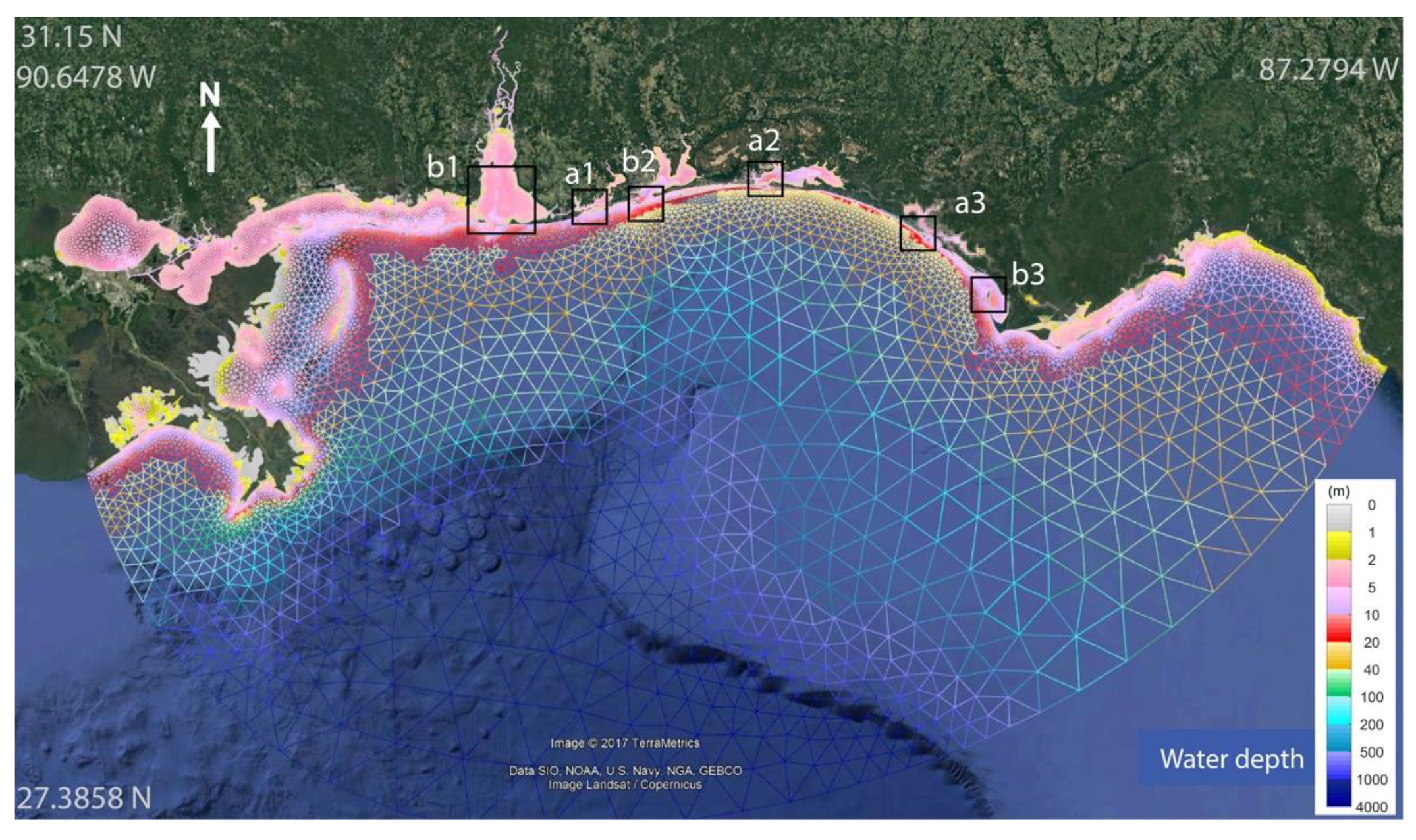
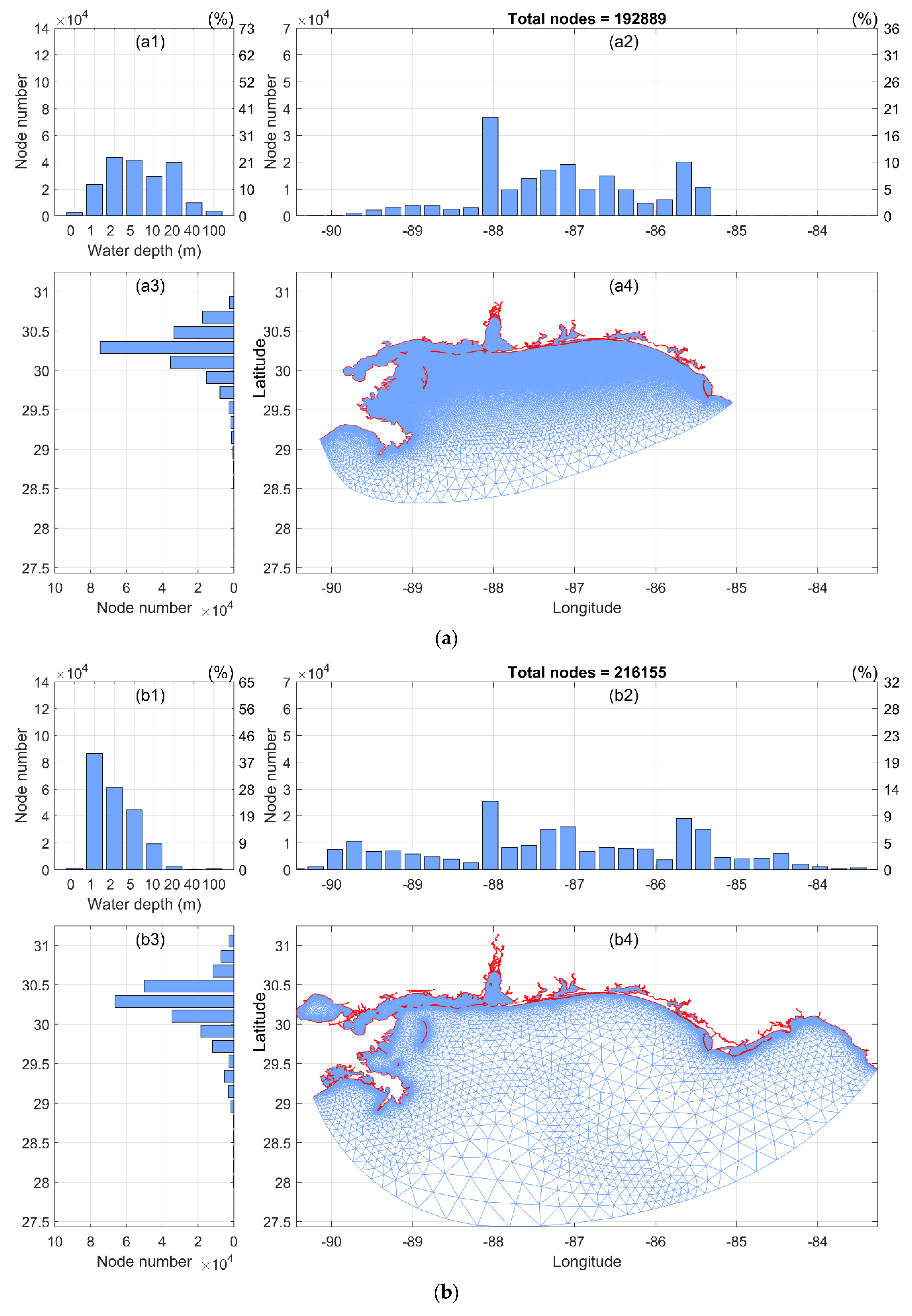
3.3. Grid Development

As illustrated in Figure 1, the mesh domain was defined by the coastline (i.e., as the land boundary) and offshore open boundary. The offshore open boundary was extended to locations with depths greater than 3000 m as well as with relatively flat bottom. The VDatum region was centered in the domain. The mainland boundary to the west was similar to the 2008 tidal model while the eastern boundary was extended further east to reduce the boundary effect to the VDatum region.

The grid development includes two main processes: (1) mesh generation and (2) water depth interpreting based on data priority. The mesh was generated by using the Surface-water Modeling System (SMS) software [39] with the size function approach. A size function is simply a collection of scatter points (in a scatter data set) that define element resolutions in different portions of the domain. It is an effective approach since it can assign high resolution only to areas that are needed, such as very shallow areas (to better resolve the non-linear wave dynamics), and coastline with high curvatures or areas with sudden changes in depth (to give a better representation of local geometry and bathymetry). We apply different criteria for defining the size function for deep ocean, nearshore, and shoreline respectively.

In the deep ocean, the dynamics of long waves are essentially governed by the shallow water approximations. That is to say, the propagation speed of tides can by approximate by $\sqrt{gd}$, where d is the depth of the ocean and g is the acceleration due to gravity. In the study, we used two parameters, wave length (L) and distance to shoreline (D), to control the size function (s). The initial resolution s₀ was set to 10 points per wave length, s₀ = L/10 = T$\sqrt{gd}$/10, where T is the wave period. Here we use T = 3 h to be on the conservative side, comparing to the typical tidal wave periods of 12 h or longer. Next we adjusted the resolution based on distance to shore based on the ratio of D to a reference distance D_ref: s = s₀ D/D_ref. In this way, for two points at the same water depth, the one closer to shore has a higher resolution. The reference distance D_ref can vary for different ocean depth. We used maximum offshore distances as D_ref at various depth contours. Here we give an example on how to generate the size function along the 1000 m depth contour. First we developed a DEM on a rectangular grid based on the bathymetry data. Next we extracted the points along the 1000 m contour line, computed D for all points along the contour, and used D_ref = max(D) at d = 1000 m. The process was repeated for different depth contours to obtain the size functions in the deep ocean.

For shallow areas and near the coastline, higher resolutions were assigned manually in SMS. We applied 60 m (or approximately 2-arc-sec) resolution for narrow breakwater entrances, 100–200 m for natural bay entrances as well as along the coastline inside bays within the VDatum region, 400 m for the relatively straight open coastline within or near the VDatum region, and 800 m for coastline areas far away from the VDatum region.

In order to provide good transition from the deep ocean to the coastline, the size function needs to be smoothed so the values (resolutions) do not change too quickly. SMS provides a toolbox to perform the smoothing task. However, some areas still need manually smoothing in addition. Such areas include locations where the open boundary connects to the mainland boundary, and narrow entrances to bays or rivers. Examples in [40] show how smoothing can enhance the poor transition from the open boundary to the mainland boundary and, therefore, improve mesh quality.

Once the model mesh was generated, the next process was to interpolate water depths onto mesh nodes based on data priority. In order to setup priority, the bathymetry data were grouped as shown in Figure 2a. Each color represents a group of data at a certain priority. The NOS survey data up to 2005 are in gray, representing the based layer of dataset which were also used to develop the 2008 tide model. NOS survey data from 2006 to 2016, which represents the new bathymetry data since the development of the 2008 tide model, were divided into three groups in yellow, green, and black colors in Figure 2a. Each group contains data subsets from different hydrographic surveys. The five filled boxes indicate the coverage of the five NCEI DEMs from 2008–2012. A boundary polygon was then developed for each group or subset. Data priority based on survey date was assigned to each boundary polygon. In general, the more recent data superseded the previous data when they overlapped.

Once boundary polygons and priority are set for all data, the mesh nodes within the boundary polygon of highest priority were then assigned a water depth value using the nearest data point from the dataset. The nearest point selection can avoid using points inside the bay/breakwaters for selecting depth for nodes outside the bay/breakwaters where the boundary polygon is in a complex shape [40]. Figure 2b displays the data sources at the mesh nodes. Figure 3 illustrates the final model grid overlapped on Google Earth. Color indicates water depth. The resolution ranges from 46 km at the open ocean boundary down to 9 m in certain sections of narrow rivers. The grid has 216,155 nodes and 374,318 elements. Figure 4 shows high resolution applied to the six inlets in the VDatum region. The inlets to Perdido Bay, Choctawahychee Bay, and Panama City have two breakwaters which further narrow the width at the entrance. Those inlets and breakwaters limit the tidal energy that can propagate into the bays.

Table 2. Properties of the 2008 and the newly-developed tide model girds.

Mesh Properties	2008	New Mesh	Increase in %
Shoreline length (km)	3979	7482	88%
Area (km2)	79,474	137,751	73%
Element number	367,019	374,318	2%
Node number	192,889	216,155	12%
Node number w/depth >20 m (percentage to total nodes)	40,545 (21%)	1777 (0.8%)	−96%
Node number w/depth 10–20 m	28,312	9721	−66%
Node number w/depth <10 m (percentage to total nodes)	124,091 (64%)	205,095 (95%)	65%

summarize the mesh properties. Compared to the 2008 mesh, the new mesh increases 88% and 73% in coverages on shoreline length and computational domain, respectively. However, the total node number increases only by 12%. This is partially due to the 96% decreas in nodes at depths greater than 20 m. Figure 5 compares the mesh and histograms between the 2008 and the new models. The two meshes have similar node distributions spatially (Figure 5 panels a2–a3 and b2–b3). However, the distributions along water depths are quite different (Figure 5 panels a1 and b1). The 2008 mesh has a relatively uniform distribution in shallow water (Figure 5(a1)) while the new mesh increases nodes sharply with decreasing water depths (Figure 5(b1)). So the new mesh represents the shallow bathymetry features more effectively. Note the nodes in deep water account only for 0.8% of the total nodes (Table 2). That is to say, we put 99.2% of the nodes in shallow water to better resolve the wave dynamics nearshore.

3.4. Model Setup

The ADCIRC model setup includes preparing the open boundary conditions and choosing parameters. The open boundary of the model grid, located in the Gulf of Mexico, was forced with a synthetic tide that was generated using the amplitude and phase of six tidal constituents (K1, O1, Q1, M2, S2, and N2), which were extracted from the East Coast 2015 (or EC2015) tidal constituent database [41]. Similar to [12], the model runs began with a smooth, hyperbolic tangent, time ramp function, which was applied to the boundary forcing tide for the first 5 days. The node factors and equilibrium arguments were set to the values from the middle of 1992, which is in the middle of the 1983–2001 NTDE. A no flow boundary was set for all main land and island boundaries. The lateral eddy viscosity coefficient was set to 5 m²/s, which was the lowest number tested that did not produce numerical instabilities. The user-specified bottom friction coefficient C_f value was set to a standard value of 0.003 as in [12]. The model was run for 40 days with a 3-s time step. The small time step was due to the Courant number limitation imposed by the small element sizes. The water surface elevation was output at every node in the grid at a 6-min time interval for the last 33 days of the 40-day model run as fort.63.nc, with a file size of 12.8 gigabytes (GB). It takes a total of 3 wall-clock hours to complete the run utilizing 256 processors at NOAA’s Research and Development High Performance Computing System’s (RDHPCS) Jet system, if we split the huge output file as two. For test runs where only time series at tide stations are needed (e.g., output fort.61.nc of 11.7 megabytes (MB) instead of fort.63.nc), it takes approximately 47 wall-clock minutes for a run. In this way, it not only saves computational resources but also improves the test efficiency.

4. Results and Discussion

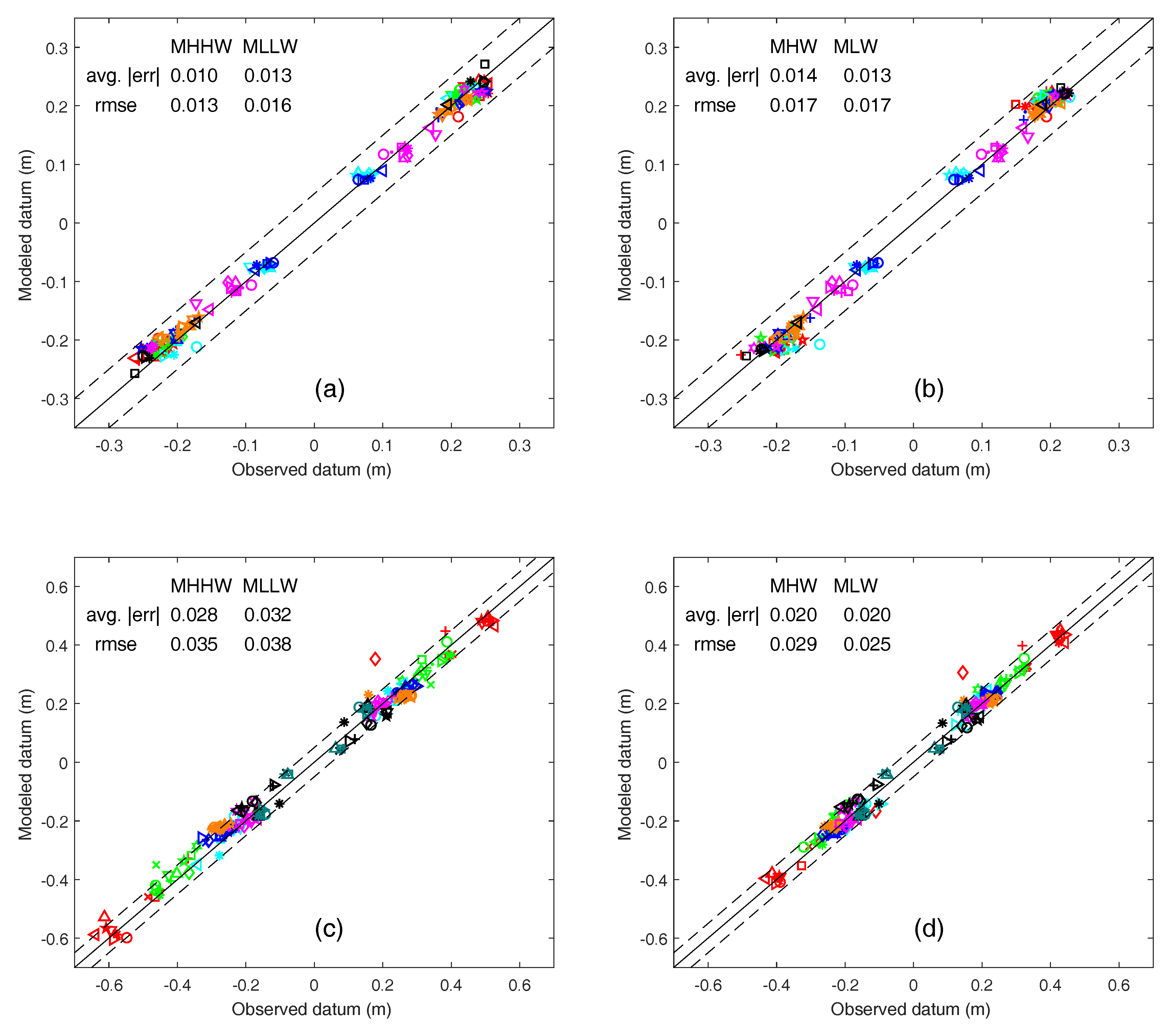
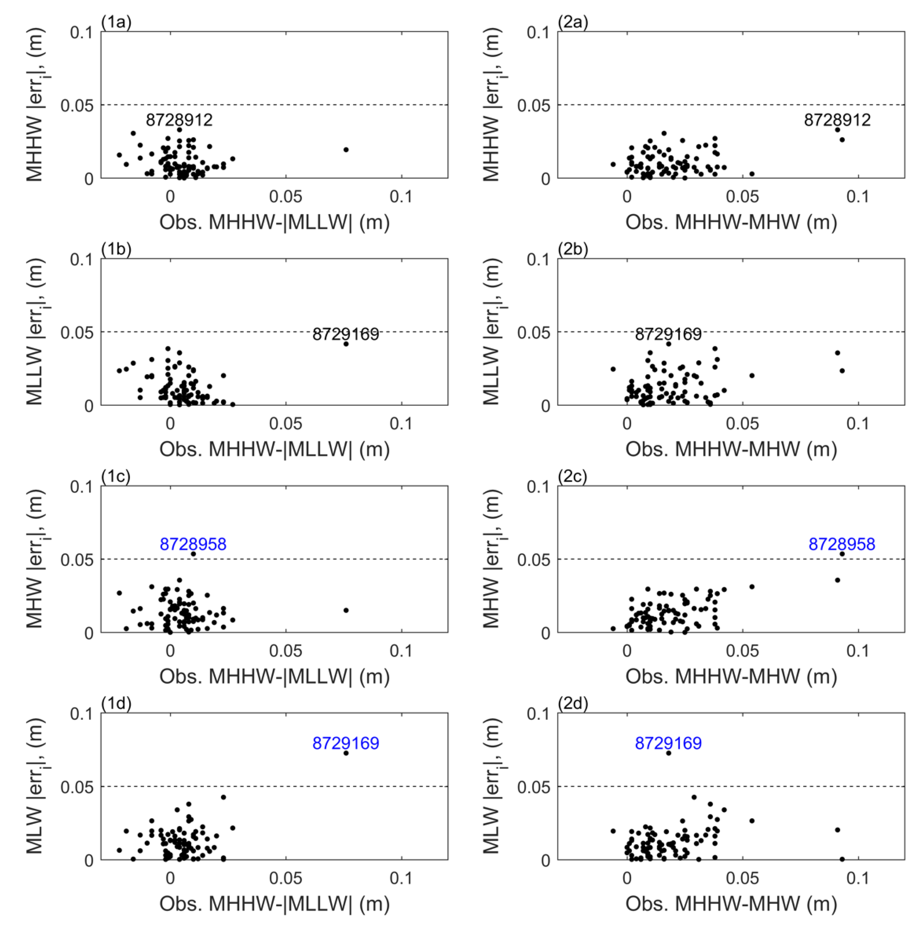
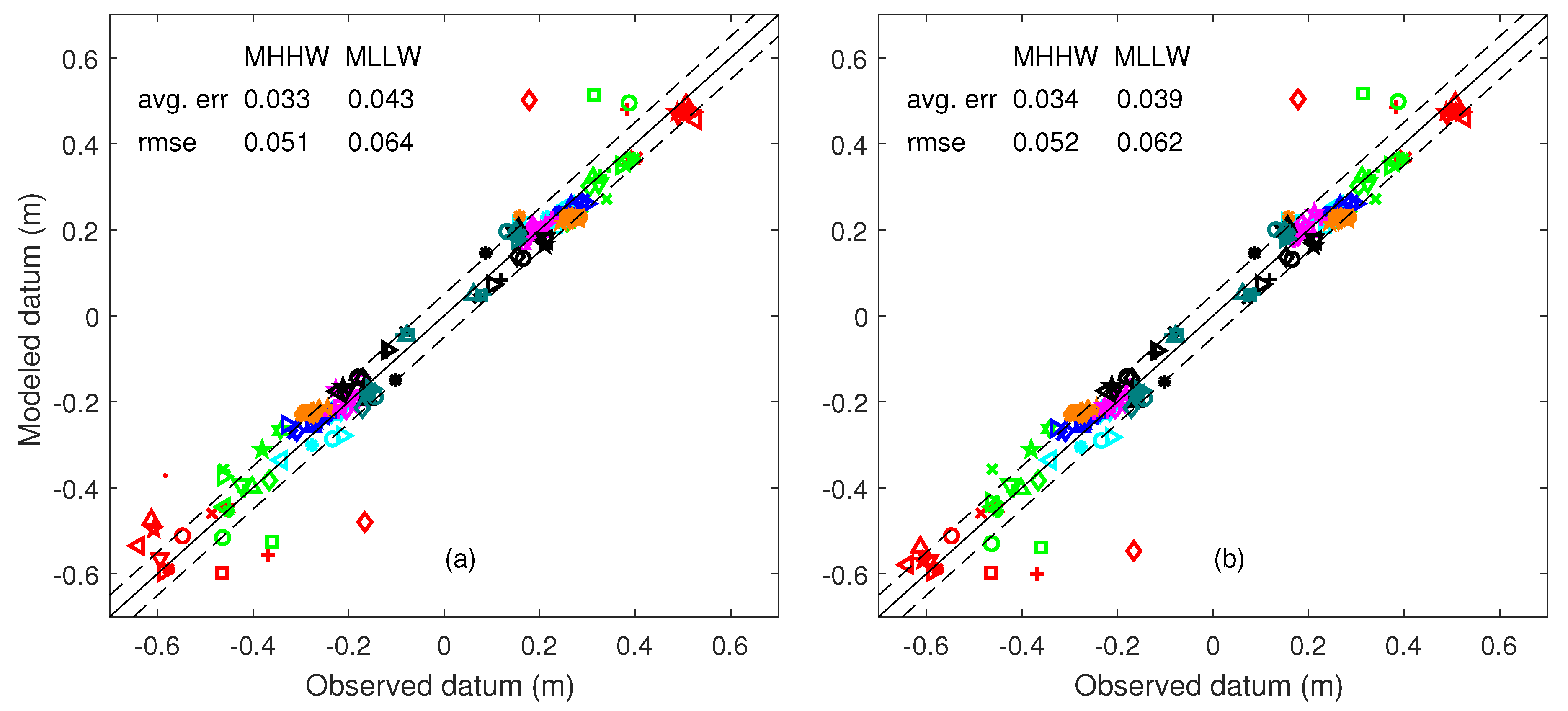
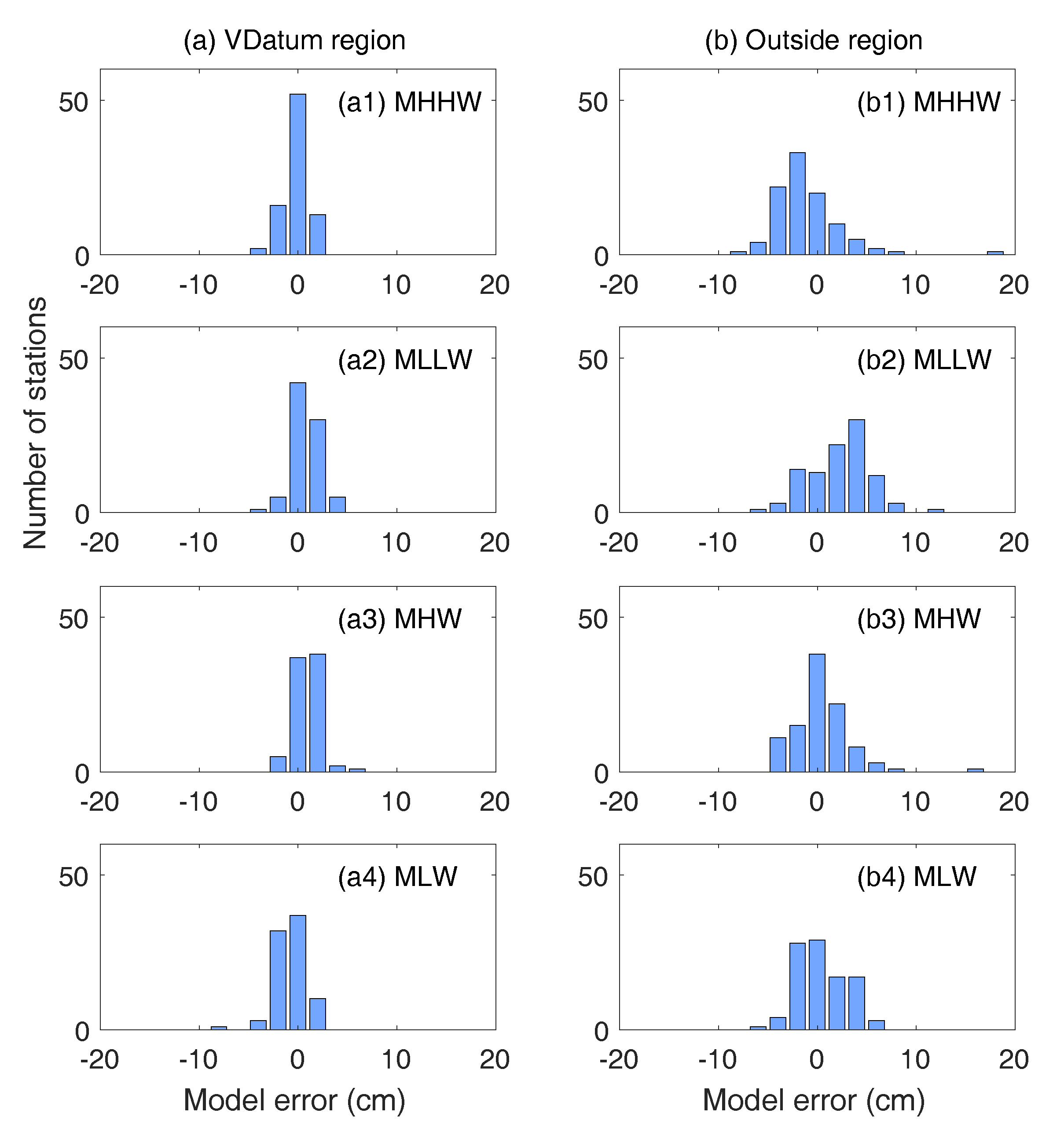
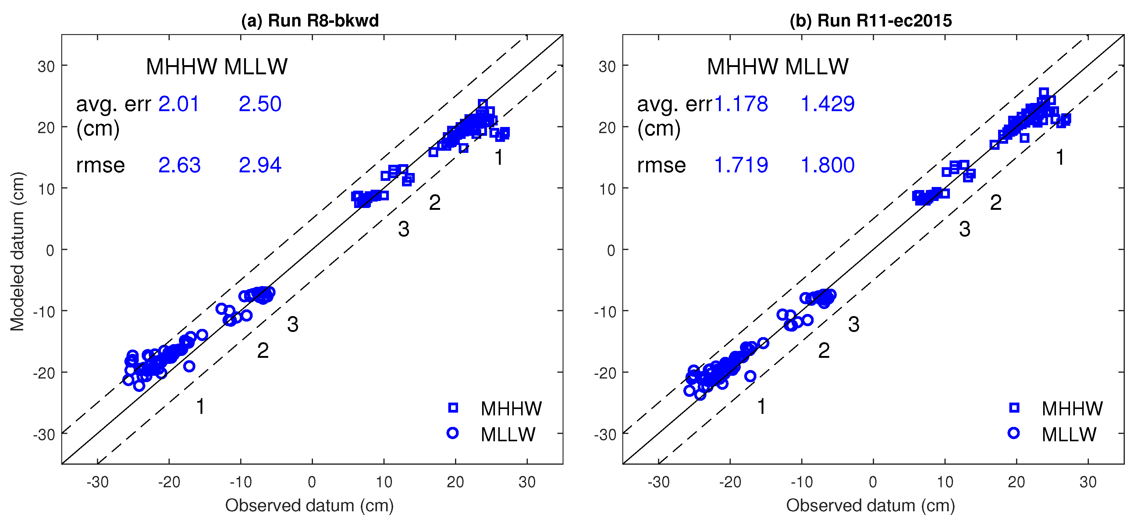
4.1. Validation and Error Analyses

In this section, we present the validation and error analyses for the original model results f_m computed from the ADCIRC model. Figure 6a–d compare the modeled datums to observations at tide stations for the four datums, MHHW, MLLW, MHW, and MLW, within and outside VDatum region, respectively.

Table 3. Summary of averaged errors, in meters, for modeled datums at tide stations for the new grid.

Tide Stations	Error	MHHW (m)	MHW (m)	MLW (m)	MLLW (m)	Four Datums (m)
83 stations in VDatum region	avg. error	0.010 6.0%	0.014 9.3%	0.013 8.9%	0.013 7.2%	0.012 7.9%
	RMSE	0.013	0.017	0.017	0.016	0.016
99 stations outside	avg. error	0.028 14.0%	0.020 12.6%	0.020 12.8%	0.032 14.2%	0.025 13.4%
	RMSE	0.035	0.029	0.025	0.038	0.032
All 182 tide stations	avg. error	0.020 10.4%	0.017 11.1%	0.017 11.0%	0.023 11.0%	0.019 10.9%
	RMSE	0.028	0.024	0.022	0.030	0.026

summarizes the model errors. Here we use obs_i and model_i for CO-OPS’ observations and the modeled datums, respectively. The model error (err_i), percentage error, average error (err_avg), and model root mean square error (rmse) are calculated as follows:

$$er{r}_i=mode{l}_i-ob{s}_i=\frac{1}{Na}{\displaystyle \sum }_{j=1}^{Na}{A}_j-ob{s}_i$$

$$\begin{gathered} \mathrm{percentage}er{r}_i=\left(mode{l}_i-ob{s}_i\right)/ob{s}_i\times 100 \\ er{r}_{avg}=\frac{1}{N}{\displaystyle \sum }_{i=1}^N\left|er{r}_i\right| \\ rmse=\sqrt{\frac{1}{N}{\displaystyle \sum }_{i=1}^{N}er{r}_i{}^2} \end{gathered}$$

where i is the ith station, A_j is the jth highs or lows from the model time series at the ith station, Na is the total number of A_j from the model time series at the ith station, and N is the number of stations used.

For the 83 tide stations within the VDatum region, the average error is 0.012 m or 7.9% for the four datums (Table 3). This is an improvement in accuracy compared to the 0.018 m (11.0%) average error for the 2008 tide model reported in [12]. As will be discussed in Section 4.3.2, the update in offshore boundary conditions from the EC2015 tidal database [41] contributes to this overall improvement. The greatest improvement is in MLLW: the average error is reduced from 0.022 m (or 12.33%) in [12] to 0.013 m (or 7.2%). Since MLLW is most sensitive to the shallow water depth among the datums, this indicates the new tide model has more accurate representation of shallow water depths in the coastal area. The results also point to another important conclusion: the gridding technique, i.e., the size function approach based on wave-lengths in the deep ocean enabled effective running of the ADCIRC model.

The model errors in the VDatum region are smaller than those outside the region. Figure 7 clearly illustrates this trend. Each bar in Figure 7 represents 2 cm in width along the x axis. In the VDatum region, 95.5% of the modeled datums have error within ±3 cm, while it is only 65.9% for the outside region. The main purpose of the outside region is to serve as a land boundary condition with relatively coarse resolution. The coarser resolution can contribute to the larger model errors.

The maximum model errors in the VDatum region are 0.033, 0.042, 0.054 and 0.073 m for MHHW, MLLW, MHW, and MLW, respectively. Two of them, MHW at station 8728958 and MLW at station 8729169, exceeded the 5-cm error band. These two stations are plotted as the red square and cyan circle respectively in Figure 6b. To explore what factors may correlate to the maximum error, we plot error against the observed differences in datum magnitude, i.e., (1) MHHW-|MLLW| and (2) MHHW-MHW, in Figure 8(1a–d,2a–d), respectively. The result indicates:

(1) The maximum errors for MLW and MHW are relatively independent. That is to say, largest errors in MLW/MLLW do not correspond with largest errors in MHW/MHHW, and vice versa. This indicates different maximum error mechanisms for MLW and MHW.

(2) The maximum errors for MLW and MLLW are highly dependent. Both are from the same station, 8729169 at Shell Point, West Bay, Fla. This indicates a similar maximum error mechanism between MLW and MLLW. This also held for the large MHW and MHHW errors at stations 8728958 and 8728912. Please refer to [40] for station numbering and locations.

(3) The maximum error for MLW/MLLW occurs when the difference in the observed MHHW and |MLLW| is the greatest. Figure 8(1d) indicates there is one such outlier station 8729169. While MHHW-|MLLW| for all other stations are less than 0.027 m, station 8729169 shows a 0.076 m difference, which is more than double of the other stations. As will discussed in Section 4.3, shallow water depth can decrease |MLLW| more effectively than MHHW, due to the greater friction at MLLW. The model and bathymetry data might not well reflect the shallow water depth around station 8729169.

(4) The maximum error for MHW/MHHW occurs when the difference in the observed MHHW and MHW is the largest. Figure 8 panels 2a and 2c indicate two such outlier stations: 8728958 and 8728912. Both are inside the Saint Joseph Bay. Station 8728958 is very close to the entrance of the Bay near the jetty area. We notice there are discrepancies between NOS survey data and the current shoreline. Some survey points with depth fall on to the land area. This indicates the bathymetry data in 1985 for the jetty area might not reflect the current shoreline and depths.

For large model errors at stations outside the VDatum region, we will have a discussion in Section 4.3 as lessons learned.

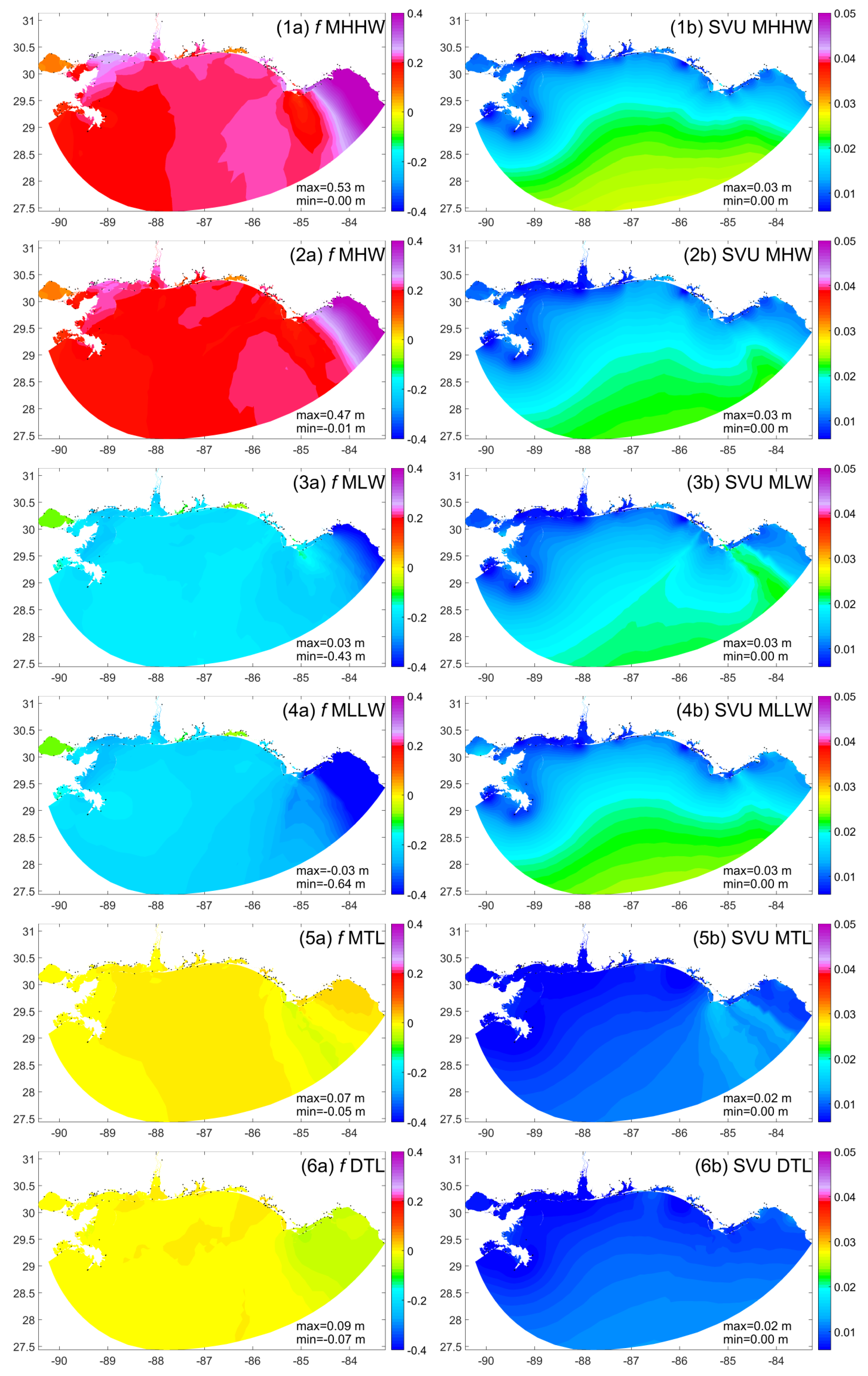
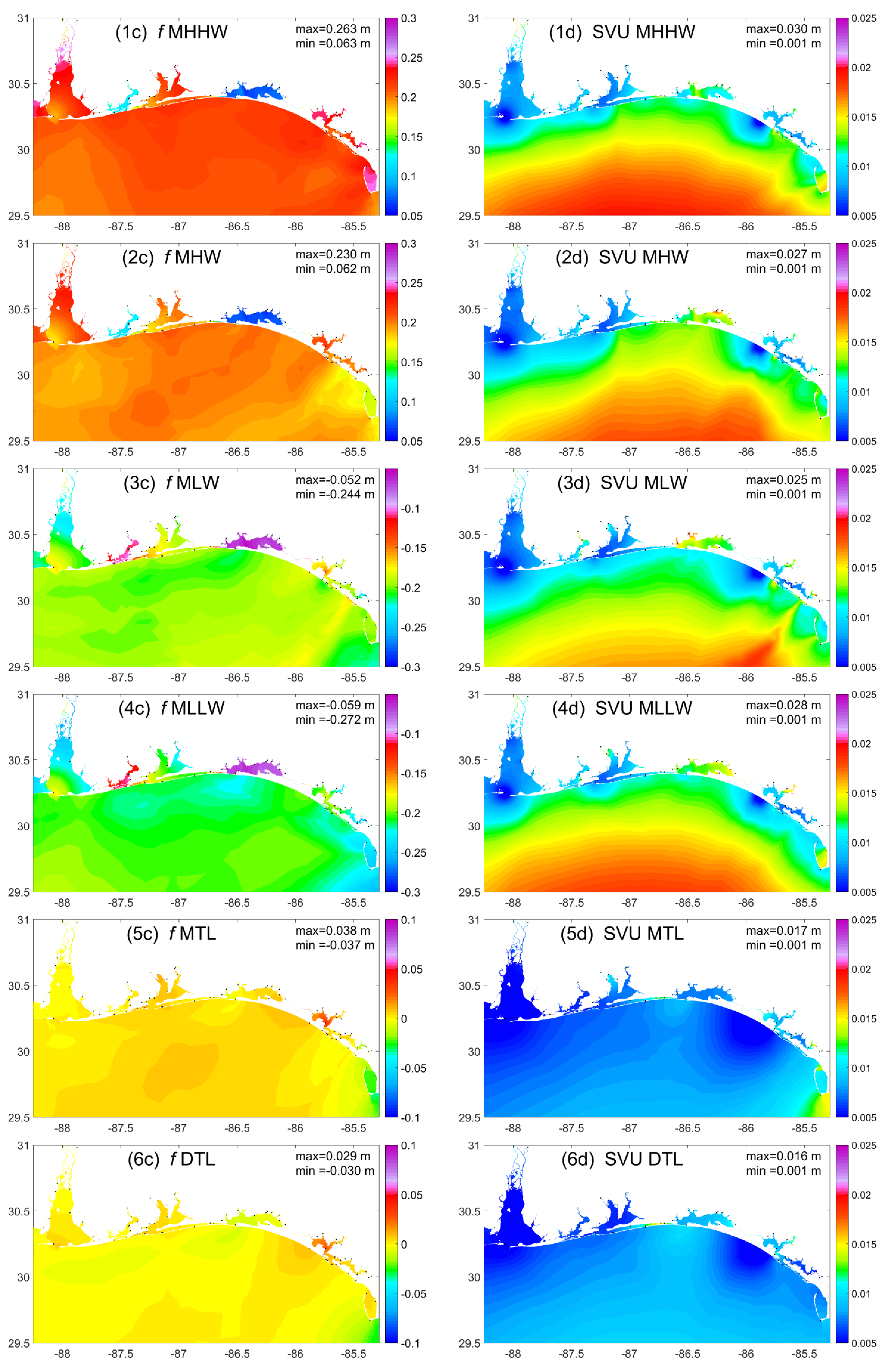
4.2. Datum Products and Spatially Varying Uncertainty

In this section, we present the results after applying the spatially varying uncertainty method. By applying the SVU method to the original model results in Section 4.1, we obtained the datum products f and associated spatially varying uncertainty Pa for the entire model domain as shown in Figure 9a,b, respectively. Rows 1–6 are for the six datum products, MHHW, MHW, MLW, MLLW, MTL, and DTL, respectively. The color map for column a ranges from −0.4 to 0.4 m while color map for column b ranges from 0 to 0.05 m. The final set of tidal datum fields match the observations at stations within a certain limit e.g., 1 cm (at the 182 tide stations in this case). The background model uncertainty had been improved at and around tide stations, and to a lesser extent in the offshore area. The maximum uncertainty is in the middle of the offshore boundary for MHHW (Figure 9(1b)). Two factors contribute to the large uncertainty offshore: (1) the lack of offshore measurements and (2) relatively farther away from tide stations in the computational domain. The uncertainty of MTL and DTL are small due to the small magnitude for these two datums.

Figure 9c,d show f and Pa in the VDatum region. The color scales in 9c and 9d were redesigned to show the local details. More details can be found in [40]. These results indicate:

(1) Along the coasts, large uncertainty can be seen in the southern portion of Saint Joseph Bay, Florida, for both MHHW and MLLW (Figure 9 panes 1d and 4d). The maximum uncertainty is 1.6 cm for MHHW. This is also the location that has the maximum MHHW and |MLLW|. Note that the MHHW-MHW and |MLLW-MLW| are also the largest among the stations in the VDatum region.

(2) For other bays, relatively local large uncertainties are found in the Choctawahatchee Bay, Florida (Figure 9 panes 2d and 3d). The maximum uncertainty ranges from 1.8 to 2.0 cm. Note that this group of tide stations inside the bay has the largest averaged measurement error even though their tidal ranges are quite small. The average measurement error is 2.7 cm inside the bay, while it is only 1.7 cm for stations in the domain.

(3) Some local large uncertainties are due to lack of measurements. Such examples include the upper stream of the Mobile River, Alabama. (1.9 cm maximum uncertainty), the Deer Point Lake, Florida, to the northern most of the Saint Andrew Bay (1.8 cm maximum uncertainty for MLLW).

(4) Large uncertainty can also be caused by the relatively large model errors. One example is the 1.9 cm maximum uncertainty and 4 cm model error for MLW at station 8728973 at Wetappo Creek, East Bay, Florida.

The above datum products and spatially varying uncertainty in VDatum region are then further interpolated and saved to five regularly spaced marine grids. Figure 10a shows the bounding polygons for the five marine grids revised by Hess in 2012 [42]. In this study, they have been further reconfigured as Figure 10b, to cover all the tide stations in the region as well as the newly-added intra-costal waterways. In addition, the bounding polygon for northwest Florida was also modified. The new polygons share the common interfaces with the adjacent polygons whenever possible, e.g., no overlaps between the polygons. By using the new polygons, new marine grids were generated for the five areas. The datum products and spatially varying uncertainty were then populated on to the new marine grids. Plots for each marine grid can be found in [40].

We next compared the VDatum values in the marine grid to the observations at the tide stations. The standard deviations range from 0.07 to 0.83 cm (

Table 4. Comparison of observations and interpolated values (Standard deviations, cm) from the marine grids for the five areas in the VDatum region.

REGION	No. of Tide Stations	MHHW	MHW	DTL	MTL	MLW	MLLW
FL_andrw03	26	0.61	0.67	0.46	0.69	0.67	0.66
FL_moble04	7	0.60	0.43	0.31	0.39	0.83	0.61
FL_negom04	4	0.42	0.57	0.36	0.5	0.75	0.65
FL_pcola03	43	0.65	0.65	0.44	0.55	0.68	0.62
FL_stjoe03	3	0.76	0.39	0.07	0.83	0.59	0.66

). The maximum error is about 1 cm. Continuity of values across interfaces was then checked. As shown in Figure 10b, there are 11 interfaces: (1) New Orleans-NEGOM, (2) New Orleans-Mobile Bay, (3) Mobile Bay-NEGOM, (4) Mobile Bay-Pensacola Bay, (5) Pensacola Bay-NEGOM, (6) Pensacola Bay-St Andrews Bay, (7) St Andrews Bay-NEGOM, (8) St Joseph Bay-NEGOM, (9) Cedar Key-NEGOM, (10) St Joseph Bay-Cedar Key, and (11) St Andrews Bay-St Joseph Bay. Along boundary 9, the NEGOM-Cedar Key boundary, there was a maximum of 2.8-cm difference in MLW across the interface. The difference is due to the differing values produced by the ADCIRC models for the north-east Gulf of Mexico and for the Florida shelf. Hess also reported a similar large difference in MLW across the 9th interface from the previous version of the tidal model [42].

4.3. Lessons Learned

In this section, we summarize lessons learned from the study to provide guidelines for future VDatum development. The modeled datums in this section refer to the original model results f_m computed from ADCIRC, i.e., before applying the spatially varying uncertainty method.

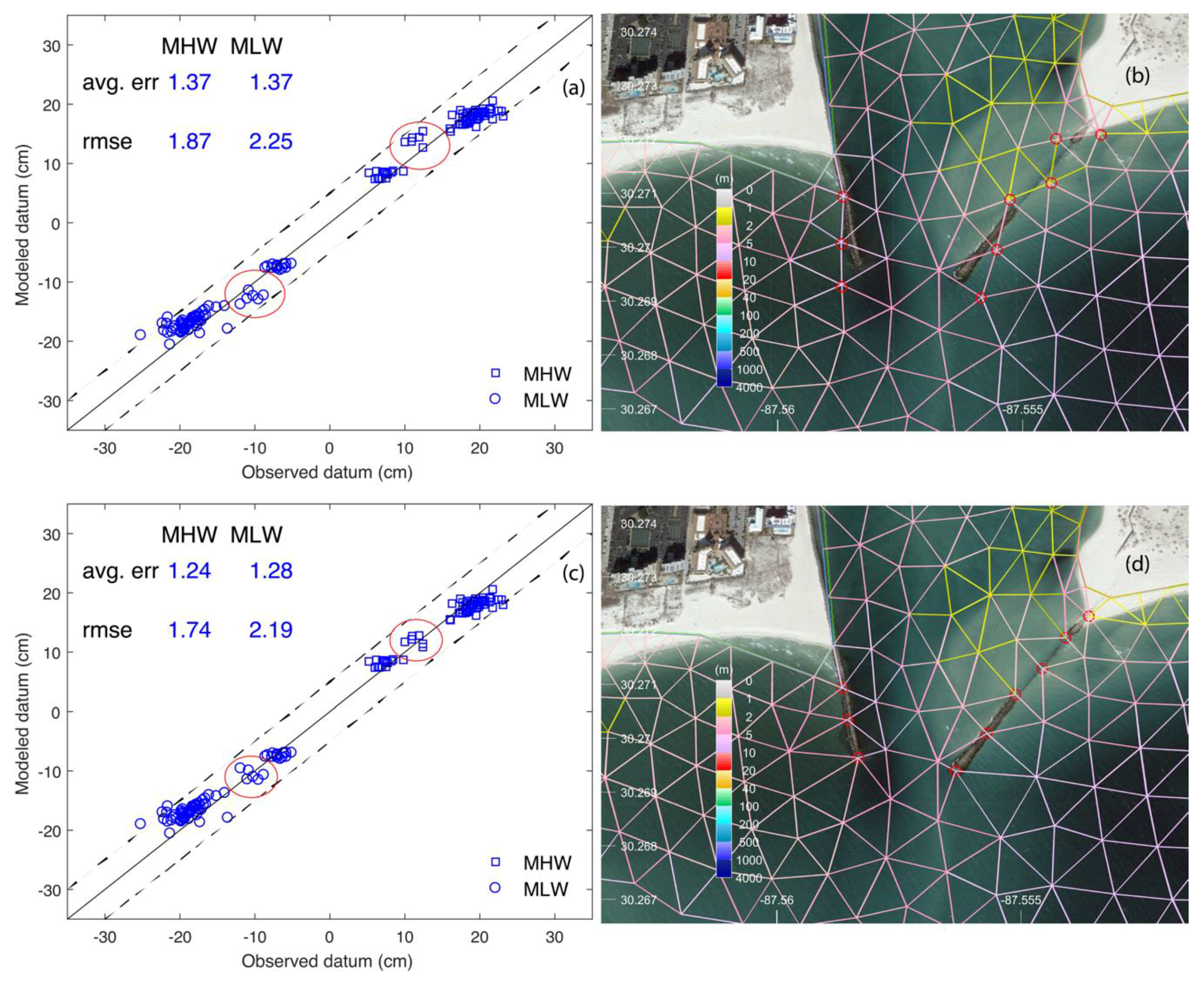
4.3.1. Sensitivity of Modeled Datums to Breakwaters

When we conducted the first test using the original 2008 model grid and input files, we obtained an over-prediction trend for stations inside Perdio Bay (Figure 11a). This is also reported by Dhingra et al. [12] in 2008, which resulted in the largest error in the Bay area. To address this issue, Dhingra et al. incorporated several changes, including extending the domain to include the lower end of the Perdido River, adding a radiation boundary condition to the upstream end of the river, and refining the intracoastal water way that connects Perdido Bay to Pensacola Bay, Fla., etc. However, no major changes in the datums resulted [12]. By overlapping the model grid on Google Earth, we found that the two breakwaters at the entrance of Perdido Bay were missing from the 2008 model grid (Figure 10b). The next test we did was to pick up 9 nodes (the red circles in Figure 11b), aligned them with the breakwaters as in Figure 11d, and assigned a land value of −1 m. Figure 11c shows the updated model results: the Perdido Bay stations now nicely distribute on both sides of the solid line, e.g., no bias. The average model errors are also reduced. The above results point to the importance of including the breakwaters at the Perdido Bay entrance for model accuracy. The 170-m-wide narrow entrance formed by the breakwaters can limit the total amount of tidal wave energy that can propagate into the Bay, thus affecting the tidal range. The model grid must resolve such sudden changes in bathymetry and coastal geometry accurately.

4.3.2. Sensitivity of Modeled Datums to Offshore Boundary Conditions

Figure 12 compares the modeled datums using the (a) EC2001 and (b) EC2015 tidal databases [24,41]. The two tests were conducted with the same 2008 model grid with 74 tide stations in the VDatum region. The EC2015 tidal database reduced errors for both MHHW and MLLW, from 2.01 and 2.5 cm to 1.18 and 1.43 cm, respectively. These represent more than 40% reduction from the original errors. The EC2015 tidal database has incorporated the bathymetry data from the VDatum tide models developed for U.S. East Coast [41]. It also has higher resolution in coastal area than the EC2001 database. Therefore, it likely has more accurate representation of the bathymetry data, particularly in shallow coastal regions. Note that the EC2015 tidal database reduced the underestimate/bais error mainly in the group 1 tide stations, which are either on the open coast or in less protected bays. Groups 2 and 3 stations in the two well-protected bays are not sensitive to the changes of offshore boundary conditions.

4.3.3. Sensitivity of Modeled Datums to Water Depth

This study also shows that water depth in coastal area plays an important role on model accuracy. Two types of very large absolute model error (>10 cm) in datums were found due to inaccurate water depths: (1) an underestimate when the water depth is not deep enough and (2) an overestimate when the water depth is too deep. Figure 13a shows these two types of errors for stations outside the VDatum region at an early stage of testing.

The first type of error (large underestimate) usually is found at |MLLW| while it has little effect on MHHW. For example, Figure 13a shows that MLLW has greater average model error than MHHW. This is due to the underestimate for some stations at MLLW only (those stations above the 5 cm error bar at MLLW in Figure 13a). An examination on the model time series at those stations reveals that at MLLW, the model outputs a non-value due to the exposure of the shallow bottom. Using high resolution bathymetry data or adjusting the water depth around the stations deeper if such data are unavailable, e.g., making them slightly deeper to avoid the bottom exposure at MLLW, improved the model results as illustrated in Figure 13b. One example is the MLLW error for station 8728130 reduced from 21 cm underestimate to 1 cm.

The second type of error (large overestimate) can affect both |MLLW| and MHHW. This usually occurs at some river stations that are not only relatively far from the open coast but also have very shallow and narrow segments, and/or with expansion and then contraction of the river width. These river features result in much smaller tidal datums than those of the stations at open coast. For example, the MHHW at station 8728171 in Wakulla River, Fla., is 0.18 m, which is significantly smaller than the 0.51 m at the nearest station 8728151. This station 8728171 has the largest model error of 0.17 m (or 98%), which is plotted as the red diamond in Figure 6 and Figure 13. Another example is the 0.38 m MHHW at station 8727989 (red plus in Figure 6 and Figure 13) in Aucilla River, Florida, which is also quite smaller than the 0.50 m MHHW at nearby stations at the open coast.

The difficulty in modeling such outlier river stations is the lack of complete, high resolution bathymetry data that can accurately represent the change of depth along the river as well as on river cross section. Examples include: there is a bathymetry data gap between NOS bathymetry data and data collected by Howard T. Odum Florida Springs Institute in Wakulla River [38]; the single beam survey data for the Aucilla River did not capture the rock section in the river [40]; there is a mismatch in position between the NOS survey data in 1878 and current NGS shoreline data in Ochlockonee River, Florida, etc. For such locations, special adjustments were applied to the river depths and widths to reduce the error as much as possible. It is based on the modeler’s best judgment, using available information from observation and bathymetry data, and Google Earth satellite imagery. Note that such adjustments are at locations within the model grid but far away from the VDatum region.

In this study, we did not tune the friction coefficient since the model accuracy in the VDatum region is already quite good. The model RMSE error for the four datums is only 1.6 cm, which is very close to the 1.7 cm averaged measurement error (RMSE) at stations. As to stations outside VDatum region with large model errors, we are in the process of obtaining more accurate bathymetry data. River LiDAR mapping projects have been conducted and proposed for Wakulla and Aucilla Rivers, respectively (personal communications with G. Cole, 2017). When those new data become available, we will redo the test for updating VDatum for those areas and evaluate the sensitivity to friction coefficients.

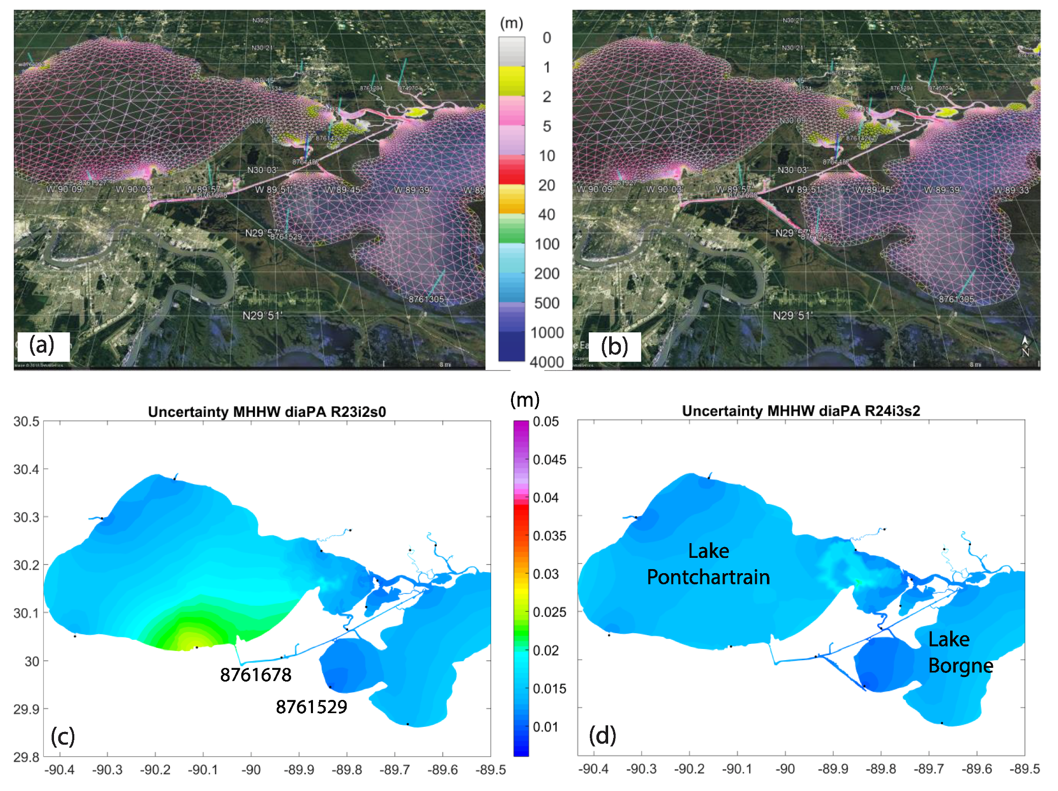
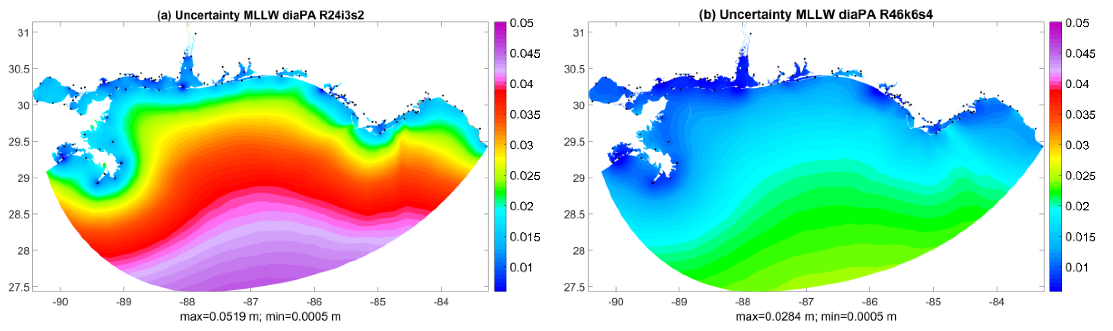
4.3.4. Sensitivity of Spatially Varying Uncertainty to Model Error

Large model errors from tide stations can propagate as background uncertainty during spatially varying uncertainty computation. Figure 14a shows the spatially varying uncertainty for MLLW using the preliminary results with large model errors as in Figure 13a. As the model error was reduced as shown in Figure 6c, the spatially varying uncertainty is also reduced as in Figure 14b. The tests were conducted using the 144 tide stations with root mean squared error data. The above results point to the importance of improving model accuracy in order to reduce the spatially varying uncertainty.

4.3.5. Model Error at Intracoastal Waterway Station 8761678

For tide stations located in the Intracoastal Waterway (ICWW), additional attention needs to be paid to the multi-connecting channels. Such an example is station 8761678, Michoud substation, ICWW, Louisiana (Figure 15). The observed MHHW and MLLW are 0.21 m at the station. Figure 15 a shows an early testing version of the grid around the station. It produces −8 cm error in both MHHW and |MLLW|. This is nearly double the −3 to −4 cm error in magnitude at the four nearby tide stations. After connecting the channel to Lake Borgne through station 8761529 (Figure 15b), the model error reduces to −4 cm for MHHW at 8761678. This is consistent with the error at the nearby tide stations. Note this reduction in error also improves the spatially varying uncertainty in the area for MHHW from Figure 15c to Figure 15d.

5. Summary and Conclusions

In this study, we highlight the creation of the tidal datum fields and associated spatially varying uncertainty for VDatum. The region of interest encompasses Mobile Bay, Ala., Perdido Bay, Ala. and Fla., Pensocola Bay, Choctawatchee Bay, St. Andrew Bay, St. Joseph Bay, and Cape San Blas, Florida, from the west to the east. We present the development, testing of the numerical model of tides in north-eastern Gulf of Mexico, and lessons learned.

In the VDatum region, the average model error is 1.2 cm (or 7.9%) for the four datums for the 83 tide stations, among which 95.5% of the modeled datums have errors within ±3 cm. After applying the spatially varying uncertainty method, the maximum absolute error in the datum products at station locations is 1 cm and the maximum uncertainty in the VDatum region is 2.5 cm. Compared to the single value uncertainty for a region, the spatially varying uncertainty provides more accurate representation of the uncertainty for the datum products.

The study points out that large model errors, measurement errors, and lack of observations can contribute to large spatially varying uncertainty. Accurate water depth data with high resolution in coastal areas is essential for improving model accuracy. This is especially important for shallow and narrow rivers. The tide model also needs to resolve the narrow entrances with breakwaters for bays well. For tide stations located in the intracoastal waterway, additional attention needs to be made to the multi-connecting channels. As we extend VDatum coverage to rivers and intracoastal waterways, high-quality river bathymetry data such as river LiDAR mapping data are needed.

The spatially varying uncertainty will be provided to the tri-office VDatum team for decision-making on placement of new tide gauges of high precision. New tide gauge data can be used to address the issues of lack of observations and large measurement errors and, therefore, to further reduce the uncertainty in the VDatum products in the future.

References

1. Parker, B. The integration of bathymetry, topography, and shoreline and the vertical datum transformations behind it. Int. Hydrogr. Rev. 2002, 3, 35–47. [Google Scholar]
2. Myers, E.P.; Wong, A.; Hess, K.; White, S.; Spargo, E.; Feyen, J.; Yang, Z.; Richardson, P.; Auer, C.; Sellars, J.; et al. Development of a national VDatum, and its application to sea level rise in North Carolina. In Proceedings of the U. S. Hydrographic Conference, San Diego, CA, USA, 29–31 March 2005. [Google Scholar]
3. USGS. National Elevation Dataset (NED)—The Long Term Archive. Available online: https://lta.cr.usgs.gov/NED (accessed on 9 October 2018).
4. Umbach, M.J. Hyrographic Manual, 4th ed.; NOAA Natioinal Ocean Service: Rockville, Maryland, 1976. [Google Scholar]
5. NOAA. NOAA/NOS’ VDatum 3.9: Vertical Datums Transformation. Available online: https://vdatum.noaa.gov/ (accessed on 9 October 2018).
6. University Colloge London. Vertical Offshore Reference Frames. Available online: https://www.ucl.ac.uk/vorf (accessed on 9 October 2018).
7. SHOM. Data.Shom.Fr. Available online: https://data.shom.fr/ (accessed on 9 October 2018).
8. Keysers, J.H.; Quadros, N.D.; Collier, P.A. Vertical Datum Transformations across the Littoral Zone; Department of Climate Change and Energy Efficiency: Canberra, Australia, 2013; p. 110. [Google Scholar]
9. NOS. Standard Procedures to Develop and Support NOAA’s Vertical Datum Transformation Tool, VDatum; Version 2010.08.03; National Ocean Service: Silver Spring, MD, USA, 2010. [Google Scholar]
10. Milbert, D.G.; Hess, K.W. Combination of topography and bathymetry through application of calibrated vertical datum transformations in the Tampa bay region. In Proceedings of the Second Biennial Coastal GeoTools Conference, Charleston, SC, USA, 8–11 January 2001. [Google Scholar]
11. CO-OPS. Computational Techniques for Tidal Datum Handbook; NOAA Special Publication NOS-OPS 2: Silver Spring, MD, USA, 2003; p. 98. [Google Scholar]
12. Dhingra, E.A.; Hess, K.W.; White, S.A. VDatum for the Northeast Gulf of Mexico from Mobile Bay, Alabama, to Cap San Blas, Florida: Tidal Datum Modeling and Population of the Marine Grids; NOAA Technical Memorandum NOS CS 14; Department of Commerce, National Oceanic and Atmospheric Administration: Silver Spring, MD, USA, 2008; p. 64. [Google Scholar]
13. Yang, Z.; Myers, E.P.; White, S.A. VDatum for Eastern Louisiana and Mississippi Coastal Waters: Tidal Datums, Marine Grids, and Sea Surface Topography; NOAA Technical Memorandum NOS CS 19; National Oceanic and Atmospheric Administration, National Ocean Service, Office of Coast Survey, Coast Survey Development Laboratory: Silver Spring, MD, USA, 2010; p. 56. [Google Scholar]
14. Xu, J.; Myers, E.P.; Jeong, I.; White, S.A. VDatum for the Coastal Waters of Texas and Western Louisiana: Tidal Datums and Topography of the Sea Surface; NOAA Technical Memorandum NOS CS 22; National Oceanic and Atmospheric Administration, National Ocean Service, Office of Coast Survey, Coast Survey Development Laboratory: Silver Spring, MD, USA, 2010. [Google Scholar]
15. Hess, K.W. Spatial interpolation of tidal data in irregularly-shaped coastal regions by numerical solution of Laplace’s equation. Estuar. Coast. Shelf Sci. 2002, 54, 175–192. [Google Scholar] [CrossRef]
16. Hess, K.W.; Schmalz, R.A.; Zervas, C.; Collier, W.C. Tidal Constituent and Residual Interpolation (TCARI): A New Method for the Tidal Correction of Bathymetric Data; NOAA Technical Report NOS CS 4; National Oceanic and Atmospheric Administration: Silver Spring, MD, USA, 1999; p. 99. [Google Scholar]
17. Hess, K.W.; Spargo, E.A.; Wong, A.M.; White, S.A.; Gill, S.K. VDatum for Central Coastal North Carolina: Tidal Datums, Marine Grids, and Sea Surface Topography; Coast Survey Development Laboratory, National Ocean Services: Silver Spring, MD, USA, 2005. [Google Scholar]
18. NOAA. NOAA/NOS’ VDatum: Estimation of Vertical Uncertainties in VDatum. Available online: https://vdatum.noaa.gov/docs/est_uncertainties.html (accessed on 9 October 2018).
19. Shi, L.; Myers, E.P. Statistical interpolation of tidal datums and computation of its associated spatially varying uncertainty. J. Mar. Sci. Eng. 2016, 4, 64. [Google Scholar] [CrossRef]
20. Fearnley, S.M.; Miner, M.D.; Kulp, M.; Bohling, C.; Penland, S. Hurricane impact and recovery shoreline change analysis of the Chandeleur Islands, Louisiana, USA: 1855 to 2005. Geo-Mar. Lett. 2009, 29, 455–466. [Google Scholar] [CrossRef]
21. Gill, S.K.; Schultz, J.R. Tidal Datums and Their Applications; NOAA Special Publication NOS CO-OPS 1; National Oceanic and Atmospheric Administration, Center for Operational Oceanographic Products and Services: Silver Spring, MD, USA, 2001; p. 111. [Google Scholar]
22. Luettich, R.A.; Westerink, J.J.; Scheffner, N.W. Adcirc: An Advanced Three-Dimensional Circulation Model of Shelves, Coasts, and Estuaries, Report 1: Theory and Methodology of Adcirc-2ddi and Adcirc-3dl.; Technical Report DRP-92-6; U.S. Department of the Army: Arlington County, VA, USA, 1992. [Google Scholar]
23. Luettich, R.A.; Westerink, J.J. Formulation and Numerical Implementation of the 2D/3D ADCIRC Finite Element Model Version 44.XX. 2004, p. 74. Available online: http://www.unc.edu/ims/adcirc/adcirc_theory_2004_12_08.pdf (accessed on 8 October 2018).
24. Mukai, A.Y.; Westerink, J.J.; Luettich R.A., Jr.; Mark, D. Eastcoast 2001: A Tidal Constituent Database for the Western North Atlantic, Gulf of Mexico and Caribbean Sea; Technical Report, ERDC/CHL TR-02-24; Coastal and Hydraulics Laboratory, US Army Engineer Research and Development Center: Vicksburg, MI, USA, 2002; p. 201. [Google Scholar]
25. Luettich, R.A.J.; Westerink, J.J. Continental Shelf Scale Convergence Studies with a Barotropic Tidal Model; American Geophysical Union Press: Washington, DC, USA, 1995; Volume 48, pp. 349–371. [Google Scholar]
26. Spargo, E.; Westerink, J.J.; Luettich, R.A.; Mark, D. Developing a tidal constituent database for the eastern north pacific ocean. In Estuarine and Coastal Modeling VIII, Proceedings of the Eighth International Conference, Monterey, CA, USA, 3–5 November 2003; American Society of Civil Engineers: Reston, VA, USA, 2004; pp. 217–235. [Google Scholar]
27. Hess, K.W.; White, S.A. VDatum for Puget Sound: Generation of the Grid and Population with Tidal Datums and Sea Surface Topography; NOAA Technical Memorandum NOS CS 4; National Oceanic and Atmospheric Administration, Coastal Survey Development Laboratory: Silver Spring, MD, USA, 2004; p. 27. [Google Scholar]
28. Michalski, M. Tide station, Tidal Datum and Geodetic Datum Assessment for VDatum Project; National Oceanic and Atmospheric Administration, Center for Operational Oceanographic Products and Services: Silver Spring, MD, USA, 2011. [Google Scholar]
29. Bodnar, A.N. Estimating Accuracies of Tidal Datums from Short Term Observations; Technical Report NOS CO-OPS 0074; National Oceanic and Atmospheric Administration, Center for Operational Oceanographic Products and Services: Silver Spring, MD, USA, 1981; p. 32. [Google Scholar]
30. National Geodetic Survey. National Geodetic Survey—NOAA Shoreline Data Explorer. Available online: https://www.ngs.noaa.gov/CUSP/ (accessed on 9 October 2018).
31. National Geodetic Survey. National Geodetic Survey Shoreline Products. Available online: https://geodesy.noaa.gov/RSD/shoredata/NGS_Shoreline_Products.htm (accessed on 9 October 2018).
32. Taylor, L.A.; Eakins, B.W.; Carignan, K.S.; Warneken, R.R.; Sazonova, T.S.; Schoollcraft, D.C.; Sharman, G.F. Digital Elevation Model of Biloxi, Mississippi, 2008b: Procedures, Data Sources and Analysis; NOAA Technical Memorandum NESDIS NGDC-9; National Oceanic and Atmospheric Administration, National Geophysical Data Center: Boulder, CO, USA, 2008. [Google Scholar]
33. Taylor, L.A.; Eakins, B.W.; Carignan, K.S.; Warneken, R.R.; Sazonova, T.; Schoollcraft, D.C.; Sharman, G.F. Digital Elevation Model of Panama City, Florida, 2008: Procedures, Data Sources and Analysis; NOAA Technical Memorandum NESDIS NGDC-8; National Oceanic and Atmospheric Administration, National Geophysical Data Center: Boulder, CO, USA, 2008; p. 27. [Google Scholar]
34. Love, M.R.; Amante, C.J.; Taylor, L.A.; Eakins, B.W. Digital Elevation Models of New Orleans, Louisiana: Procedures, Data Sources and Analysis; NOAA Technical Memorandum NESDIS NGDC-49; National Oceanic and Atmospheric Administration, National Geophysical Data Center: Boulder, CO, USA, 2011; p. 46. [Google Scholar]
35. Love, M.R.; Caldwell, R.J.; Carignan, K.S.; Eakins, B.W.; Taylor, L.A. Digital Elevation Models of Southern Louisiana: Procedures, Data Sources and Analysis; National Oceanic and Atmospheric Administration, National Geophysical Data Center: Boulder, CO, USA, 2010; p. 22. [Google Scholar]
36. Love, M.R.; Amante, C.J.; Carignan, K.S.; Eakins, B.W.; Taylor, L.A. Digital Elevation Models of the Northern Gulf of Coast: Procedures, Data Sources and Analysis; National Oceanic and Atmospheric Administration, National Geophysical Data Center: Boulder, CO, USA, 2010. [Google Scholar]
37. DeWitt, N.C.; Stalk, C.A.; Smith, C.G.; Locker, S.D.; Fredericks, J.J.; McCloskey, T.A.; Wheaton, C. Single Beam Bathymetry Data Collected in 2015 from Grand Bay, Mississippi/Alabama; United States Geological Survey: Reston, VA, USA, 2015. [Google Scholar]
38. The Howard, T. Odum Florida Springs Institute. Wakulla Springs Baseline Ecosystem Assessment; Florida Springs Institute: High Springs, FL, USA, 2016; p. 101. [Google Scholar]
39. AQUAVEO. Aquaveo: Water Resources Software and Engineering Consulting Services for Modeling Groundwater, Surface-Water, and Watershed Hydraulics & Hydrology. Available online: https://www.aquaveo.com/ (accessed on 9 October 2018).
40. Tang, L.; Myers, E.P.; Shi, L.; Hess, K.; Carisio, A.; Michalski, M.; White, S.A.; Hoang, C. VDatum with Spatially Varying Uncertainty in the Northeast Gulf of Mexico from Mobile Bay, Alabama, to Cape San Blas, Florida; NOAA Technical Report NOS CS; National Oceanic and Atmospheric Administration: Silver Spring, MD, USA, 2018; p. 79. [Google Scholar]
41. Szpilka, C.; Dresback, K.; Kolar, R.; Feyen, J.; Wang, J. Improvements for the western north atlantic, caribbean and gulf of mexico adcirc tidal database (EC2015). J. Mar. Sci. Eng. 2016. [Google Scholar] [CrossRef]
42. Hess, K.W. Revised VDatum for the northeast gulf of Mexico. Unpublished work. 2012; 7. [Google Scholar]
Figure 1. VDatum region (red box) and computational domain for the new tide model for the north-east Gulf of Mexico. Red and cyan bars represent the observed MHW at tide stations within and outside the VDatum region, respectively. As a reference, the first bar from the east represents MHW of 0.41 m. Yellow and white lines are the shoreline and open boundary of the computational domain, respectively. White box indicates the location of NEGOM. Background images are from Google Earth.
Jmse 06 00114 g001
Figure 2. (a) Major bathymetry data sources overview. Data priority is based on survey date. The more recent data, the higher data priority. (b) Bathymetry data sources at mesh nodes.
Jmse 06 00114 g002
Figure 3. The newly developed tidal model grid for north-east Gulf of Mexico. Colors indicate water depth in meter. See Figure 4 for the close-ups in the boxes. Background image is from Google Earth.
Jmse 06 00114 g003
Figure 4. High resolution applied at six inlets to Bays in VDatum region. (a) Three narrow inlets with breakwaters. (b) Three nature inlets. See Figure 3 for locations.
Jmse 06 00114 g004
Figure 5. Comparison of the (a) 2008 and (b) new model meshes. (13) Histograms of node number versus depth, longitude, and latitude, respectively.
Jmse 06 00114 g005
Figure 6. Comparison of the modeled tidal datum and observations for tide stations (a,b) within and (c,d) outside the VDatum region. The dashed lines indicate the 5-cm error band.
Jmse 06 00114 g006
Figure 7. Histograms of model errors for tide stations (a) in and (b) outside the VDatum region.
Jmse 06 00114 g007
Figure 8. Model errors for (a) MHHW, (b) MLLW, (c) MHW, and (d) MLW versus observed differences in magnitude of (1) MHHW and MLLW, and (2) MHHW and MHW for stations in the VDatum region.
Jmse 06 00114 g008
Figure 9. Datums products f and associated spatially varying uncertainty Pa in (a,b) computational domain and (c,d) VDatum region. Rows (16) are the six datums, MHHW, MHW, MLW, MLLW, MTL, and DTL, respectively.
Jmse 06 00114 g009aJmse 06 00114 g009b
Figure 10. (a) 2012 and (b) 2018 revised bounding polygons. Dots indicate the locations of the tide stations.
Jmse 06 00114 g010
Figure 11. (a,c) Model data comparison at 74 stations in VDatum region (b) without and (d) with breakwaters at the entrance, respectively. Tide stations inside the Perdido Bay were within the red circle. Tests were conducted using the 2008 model grid. The dashed lines indicate the 5-cm error band.
Jmse 06 00114 g011
Figure 12. Sensitivity of modeled datums to offshore boundary conditions using (a) EC2001 and (b) EC2015 tidal data base. Tests were conducted using the 2008 model grid with breakwaters added to Perdido Bay. The dashed lines indicate the 5-cm error band.
Jmse 06 00114 g012
Figure 13. Sensitivity of modeled datum to water depth for stations outside VDatum region. (a) Two types of large model error at early stage of testing. (b) Increasing minimum water depth resolved the underestimate at MLLW. See Figure 6c for the final results. The dashed lines indicate the 5-cm error band.
Jmse 06 00114 g013
Figure 14. Sensitivity of spatially varying uncertainty to model error. (a) Before and (b) after error reduction (e.g., Figure 13a vs. Figure 6c). Tests were conducted using 144 tide stations with RMSE data. Unit for the color bar is in meter.
Jmse 06 00114 g014
Figure 15. Sensitivity of spatially varying uncertainty to model error at intracoastal waterway station 8761678. (a) 8 cm and (b) 4 cm error at 8761678, Michoud substation, Intracoastal Waterway (ICWW), Louisiana. (c) and (d) Spatially varying uncertainty computed from the model grids in (a) and (b), respectively.
Jmse 06 00114 g015