Parameterized Airfoil Design and Optimization for Vertical-Axis Tidal Turbines

Abstract

This study presents a systematic airfoil optimization framework to enhance the hydrodynamic performance of vertical-axis tidal turbines (VATTs) under low-flow conditions. The integrated methodology combines parameterized design, response surface methodology (RSM) optimization, and high-fidelity computational fluid dynamics (CFD) validation to investigate the effects of maximum thickness (Factor A), maximum thickness position (Factor B), and maximum camber (Factor C). The shear stress transport (SST) k-ω turbulence model was employed for flow simulation, with experimental validation conducted across Reynolds numbers from 5.2 × 10⁵ to 8.6 × 10⁵. The tip speed ratio (TSR) predictions demonstrated excellent agreement with experimental measurements, showing a maximum relative error of only 4.5%. From hundreds of Pareto-optimal solutions, five candidate designs were selected for high-fidelity verification. The final optimized airfoil (Optimized Foil 5) achieved a power coefficient (C_P) of 0.1887, representing a 27.5% improvement over the baseline National Advisory Committee for Aeronautics (NACA) 2414 airfoil. This optimal configuration features 23.51% maximum thickness, 30.14% maximum thickness position, and 3.99% maximum camber, with only 0.2% deviation between RSM prediction and CFD validation. The research establishes a reliable design framework for VATTs operating in low-velocity tidal streams, providing significant potential for harnessing previously uneconomical marine energy resources.

1. Introduction

The geometric parameters of vertical-axis tidal turbine (VATT) blades decisively govern their low-velocity performance. Studies demonstrate that airfoil camber significantly enhances starting torque, with 20% camber blades increasing the power coefficient by up to 24.42% [1]. Conversely, thickness parameters regulate stall characteristics—thinner profiles (14% thickness) outperform thicker counterparts (18% thickness) in pre-stall lift-to-drag ratio but suffer 41% performance degradation post stall [2]. Current optimization strategies include coupled curvature-pitch angle design [3,4], counter-rotating rotor configurations [5,6,7], and composite material applications [8]. Among these, response surface methodology and neural networks (e.g., TurbineNet) achieve ≤2% errors in hydrodynamic prediction [9]. Nevertheless, the influence of blade geometry on startup vortex evolution mechanisms remains unquantified [10], hindering adaptability in low-velocity conditions.

Wake recovery velocity directly determines array energy capture efficiency. Ducted turbine wakes conform to a double-Gaussian model with accelerated recovery [11], while staggered array layouts enhance wake recovery by 10%~21% compared to square arrangements [12,13,14]. Environmental perturbations exhibit complex dynamics: waves amplify torque fluctuations threefold [15]; seabed topography causes ±40% power output variations [16,17]; sediment-laden flows alter lift–drag coefficients [18]; and support structures trigger local scouring [19]. To address these, array controllers stabilize loads by regulating pitch angles and rotational speeds [20,21], and quantum discrete particle swarm optimization improves power generation by 19%. However, existing wake models lack experimental validation under wave–current coupling [22,23,24], limiting their engineering applicability.

High-fidelity numerical simulation is central to performance prediction. Large eddy simulation resolves unsteady vortex shedding [25], while the SST k-ω model achieves <9.2% error in stall prediction [26]. Fluid–structure interaction models (e.g., DLFSI [27]) optimize blade stress distributions. Experimentally, particle image velocimetry (PIV) quantifies near-wake structures [28], and vessel-mounted ADCP characterizes megawatt-scale turbine wakes [29]. Yet limitations persist: blade element momentum theory fails to resolve dual-rotor interference; RANS models exhibit >15% deviations in separated flow prediction [30]; and scaled experiments struggle to replicate real-sea turbulence intensity. Crucially, high-resolution validation of startup vortex evolution remains scarce [31].

This study addresses this critical gap by establishing an integrated research framework combining parametric airfoil design, response surface optimization, and high-fidelity CFD verification. Unlike previous comparative studies of existing airfoils, our approach systematically explores the design space through three key geometric parameters: maximum thickness ratio (Factor A), location of maximum thickness (Factor B), and maximum camber (Factor C). This methodology enables the identification of optimal airfoil configurations specifically tailored for low-velocity tidal conditions (Reynolds number = 1.6 × 10⁶).

Our contribution advances the field in three significant aspects: (1) development of a parameterization scheme that efficiently captures the geometric characteristics most influential to low-Reynolds number performance; (2) implementation of response surface methodology to navigate the complex multi-parameter design space while minimizing computational cost; and (3) rigorous validation through three-dimensional unsteady simulations that capture the dynamic flow phenomena characteristic of vertical-axis turbines. The optimization framework identifies an airfoil configuration that achieves a 27.5% improvement in power coefficient compared to the baseline NACA 2414 design.

The structure of this paper is organized as follows: Section 2 details the parametric design methods and computational framework, including model establishment, meshing, numerical model setup, and experimental validation methods; Section 3 presents the optimization process and validation results, analyzes the influence mechanisms of airfoil parameters on performance, and discusses the research limitations and future work directions; Section 4 summarizes the main research conclusions.

2. Methodology

2.1. Model Establishment and Meshing

2.1.1. Three-Dimensional Computational Domain Setup

Based on the parameters listed in Table 1, a three-dimensional model of the vertical-axis tidal current turbine was constructed, as shown in Figure 1. A three-dimensional computational domain for the vertical-axis tidal current turbine was established according to the parameters in Table 2. The domain consists of a stationary zone and a rotating zone, illustrated in Figure 2.

Table 1. Turbine Model Parameters.

Turbine Model Parameter Name	Turbine Model Parameter Value (m)
Central Rotating Shaft Diameter	0.03
Central Rotating Shaft Height	0.2
Rotor Radius	0.4
Blade Chord Length	0.2
Blade Height	0.4
Rotating Bracket Thickness	0.008

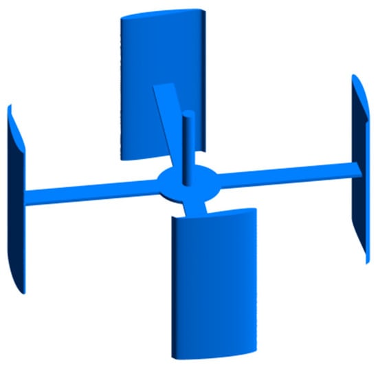
Figure 1. Three-Dimensional Model.

Table 2. Parameters of the Three-Dimensional Computational Domain.

Parameter Name of the Three-Dimensional Computational Domain	Parameter Dimension (m)
Stationary Domain Length	4.5
Stationary Domain Width	1.6
Stationary Domain Height	1.6
Rotating Domain Diameter	1.2
Rotating Domain Height	0.8
Distance from Inlet to Rotor Center	1.5

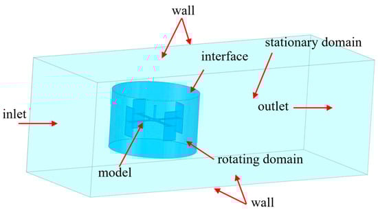
Figure 2. Three-Dimensional Computational Domain.

2.1.2. Three-Dimensional Meshing

For the meshing of the three-dimensional computational domain, an unstructured mesh was generated, as shown in Figure 3. The computational domain was divided into a stationary zone and a rotating zone, connected via an interface to ensure overall mesh quality. Mesh quality constraints were applied to enhance the quality of the mesh in critical regions, as detailed in Table 3. For the surfaces of the blades and support structures, this model employs high-quality unstructured mesh refinement instead of traditional prismatic layer meshes. During preprocessing for vertical-axis turbines with complex three-dimensional rotating domains and sharp junctions, it was found that generating high-quality prismatic layer meshes with sufficient layers often leads to cell distortion or negative volumes, resulting in non-convergent calculations. To ensure result reliability, this study adopted an alternative approach by strictly controlling the height of the first layer of mesh, ensuring that the wall (Y+) values across the entire domain fall within the viscous sublayer range applicable to the SST k-ω turbulence model (Y+ = 1–5). The good agreement in mesh independence verification (Section 2.3) and experimental validation (Section 3.1) demonstrates that the current mesh strategy can accurately capture boundary layer physics, providing a reliable foundation for subsequent optimization analysis.

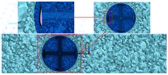
Figure 3. Mesh of the 3D Computational Domain.

Table 3. Mesh Quality Parameters of the 3D Computational Domain.

Mesh Quality Parameter Name	Mesh Quality Parameter Value
Minimum Orthogonal Quality	0.3
Average Orthogonal Quality	0.8
Maximum Aspect Ratio	13.88
Number of Isolated Cells	0

2.2. Numerical Model and Boundary Condition Setup

2.2.1. Mathematical Equations

For the three-dimensional numerical simulation, the torque value M is obtained from the numerical simulation software Fluent 2024 R1. The average torque M_avg over five stable operating cycles is calculated as follows:

$$M_{avg}={\displaystyle \frac{1}{5T}}{\displaystyle {\int }_{t_0}^{t_0+5T}M}\left(t\right)dt$$

(1)

where t₀ is the start time of the stable phase and T is the rotational period of the rotor, given by:

$$T={\displaystyle \frac{2\pi }{\omega }}$$

(2)

where ω is the angular velocity of the rotor.

Subsequently, the output power P_out and the power coefficient C_P of the rotor are calculated using the following formulas:

$$P_{out}=M\times \omega$$

(3)

$$C_P={\displaystyle \frac{P_{out}}{P_{in}}}$$

(4)

Here, P_in is calculated based on the hydrodynamic parameters, expressed as:

$$P_{in}={\displaystyle \frac{1}{2}}\rho A{V}^3$$

(5)

where ρ is the water density, A is the swept area of the rotor, and V is the flow velocity.

Furthermore, to better describe the rotor motion, the tip speed ratio TSR is introduced, defined as:

$$TSR={\displaystyle \frac{\omega R}{V}}$$

(6)

2.2.2. Turbulence Equation

Through integrating the Standard k-ω model and Standard k-ε model, Mentor et al. developed the Baseline model (designated as BLS model), which incorporates the advantages of both original models. Building upon this newly established BLS framework, a functional relationship between turbulent kinematic viscosity coefficient and Reynolds stress was formulated, leading to the derivation of the SST k-ω model. The governing equations of the SST k-ω model are expressed as follows:

$${\displaystyle \frac{\partial \left(\rho u_{j}k\right)}{\partial x_j}}+{\displaystyle \frac{\partial \left(\rho k\right)}{\partial t}}={\displaystyle \frac{\partial }{\partial x_j}}\left[{\displaystyle \frac{\partial k}{\partial x_j}}\left({\displaystyle \frac{{\mu }_t}{{\mathrm{\sigma }}_{ks}}}+\mu \right)\right]+P_k-\rho {\beta }^{*}k\omega$$

(7)

$$\begin{array}{l}{\displaystyle \frac{\partial \left(\rho u_j\omega \right)}{\partial x_j}}+{\displaystyle \frac{\partial \left(\rho \omega \right)}{\partial t}}={\displaystyle \frac{\partial }{\partial x_j}}\left[{\displaystyle \frac{\partial \omega }{\partial x_j}}\left({\displaystyle \frac{{\mu }_t}{{\mathrm{\sigma }}_{\infty 3}}}+\mu \right)\right]\\ +2\left(1-F_1\right)\rho {\mathrm{\sigma }}_{w2}{\displaystyle \frac{1}{\omega }}{\displaystyle \frac{\partial k}{\partial x_j}}{\displaystyle \frac{\partial \omega }{\partial x_j}}+a_3{P}_k{\displaystyle \frac{\omega }{k}}-{\beta }_3\rho {\omega }^2\end{array}$$

(8)

$$P_k={\mu }_t{\displaystyle \frac{\partial u_i}{\partial x_j}}\left({\displaystyle \frac{\partial u_i}{\partial x_j}}+{\displaystyle \frac{\partial u_j}{\partial x_i}}\right)-{\displaystyle \frac{2}{3}}{\displaystyle \frac{\partial u_k}{\partial x_k}}\left({\mu }_t{\displaystyle \frac{\partial u_j}{\partial x_i}}+\rho k\right)$$

(9)

The SST k-ω model comprehensively accounts for turbulent shear stress, demonstrating superior applicability in computational analysis of flow separation phenomena. For tidal energy turbine flow characteristics analysis, this model delivers high-fidelity results. Consequently, the present study adopts this turbulence model.

2.2.3. Boundary Condition Setup

A pressure-based transient solver was employed for the numerical simulations, as it can capture the dynamic fluctuations of the turbine within the flow field. The working fluid was liquid water, with density and dynamic viscosity set to 998.2 kg/m³ and 0.001003 kg/(m·s), respectively. The corresponding inflow velocity was 2.0 m/s, resulting in a Reynolds number of 1.6 × 10⁶. This flow velocity condition is based on typical low-velocity tidal energy resource environments (commonly found in estuaries or coastal areas) and is aimed at optimizing the performance of vertical-axis tidal turbines in such widespread yet underdeveloped low-energy flow fields. The boundary conditions for the computational domain were set as velocity inlet and pressure outlet. The SST k-ω turbulence model was selected due to its capability to accurately capture flow separation phenomena. Computation was considered convergent when residuals for all governing equations dropped below 10⁻³ and key performance parameters stabilized.

Regarding boundary conditions for the numerical simulation, a sliding mesh approach was adopted. A fixed tip speed ratio (TSR) of 1.256 was set, corresponding to a rotational speed ω = 6.28 rad/s. This setup aimed to identify the airfoil rotor configuration with the highest aerodynamic efficiency under specified conditions.

Additionally, a dynamic mesh technique was used to simulate the turbine’s rotation under natural conditions, allowing comparison with experimental results to validate the reliability of the numerical simulation. A 6DOF (six degrees of freedom) solver was utilized, permitting the rotor to freely rotate about its axis under hydrodynamic influences. The mass and moment of inertia of the turbine model were specified for the 6DOF calculation to ensure the accuracy of rotor performance data.

2.3. Grid Independence Verification

2.3.1. Grid Independence Verification Method

Based on the simulation data, Richardson extrapolation was used to estimate the exact value, expressed as:

$$f_{exact}=f_{fine}+{\displaystyle \frac{f_{fine}-f_{medium}}{r^p-1}}$$

(10)

where f_exact, f_fine, f_medium denote the extrapolated value, fine grid value, and medium grid value, respectively; r is the grid refinement ratio; and p is the order of convergence.

The error Δ between the extrapolated value and the fine grid value is then calculated as:

$$\mathrm{\Delta }={\displaystyle \frac{\left|f_{exact}-f_{fine}\right|}{\left|f_{exact}\right|}}$$

(11)

Subsequently, the Grid Convergence Index (GCI) is computed as:

$$GC{I}_{fine}=F_S\times {\displaystyle \frac{\left|f_{fine}-f_{medium}\right|/\left|f_{fine}\right|}{r^p-1}}$$

(12)

where F_S is the safety factor.

2.3.2. Three-Dimensional Grid Independence Verification

By halving the meshing parameters, three grid systems were constructed with cell counts of 610,000, 1.97 million, and 7.17 million, respectively. The operational performance of a turbine with NACA 2414 blade airfoils was simulated under a Reynolds number of 1.6 × 10⁶. The calculation results are shown in Table 4.

Table 4. Three-Dimensional Grid Calculation Results.

Number of Grid Cells	Angular Velocity ω (rad/s)
610,000	9.01
1.97 million	9.51
7.17 million	9.56

Assuming second-order accuracy, an extrapolated estimate of ω = 9.58 rad/s was obtained for an infinitely refined grid. The relative error between the result from the 1.97 million-cell grid and the extrapolated value was 0.7%, which is below the commonly used engineering error threshold. This indicates that this grid density sufficiently captures flow field characteristics and ensures the grid independence of the calculation results.

The Grid Convergence Index (GCI) was further calculated using a safety factor F_S = 1.25. The GCI values based on different grid counts were 2.19% and 0.22%, respectively. The GCI value for the 7.17 million-cell grid relative to the 1.97 million-cell grid was below 2%, indicating a high degree of grid convergence for the numerical solution. Further grid refinement would not cause unacceptable fluctuations in the solution.

Therefore, all subsequent 3D numerical simulations employed a grid system with approximately 1.97 million cells.

2.4. Introduction to the Experimental Setup

2.4.1. Prototype and Experimental Setup

This experimental validation aims to confirm that the established 3D CFD model possesses reliable accuracy in predicting the overall performance of the turbine. This provides a credible foundation for the parametric study and optimization based on this CFD method in the next section.

The physical model assembled for validation is a 1:1 prototype of the VATT, featuring four blades with the NACA 2414 airfoil. A rotational speed sensor was used to monitor the rotor speed, connected to the turbine rotor shaft via a diaphragm coupling, as shown in Figure 4. Key geometric parameters are consistent with the numerical model parameters listed in Table 1.

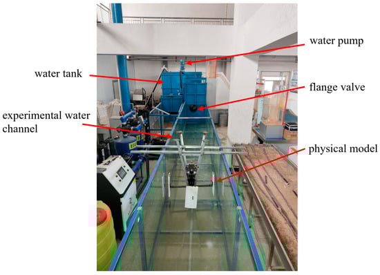
Figure 4. Photograph of the Physical Model.

The experiment was conducted in a circulating water channel, as illustrated in Figure 5, with its parameter dimensions matching those in Table 2. The turbine was installed in the mid-to-rear section of the channel via a rigid support structure to obtain a relatively stable flow environment while ensuring the turbine rotor was fully submerged.

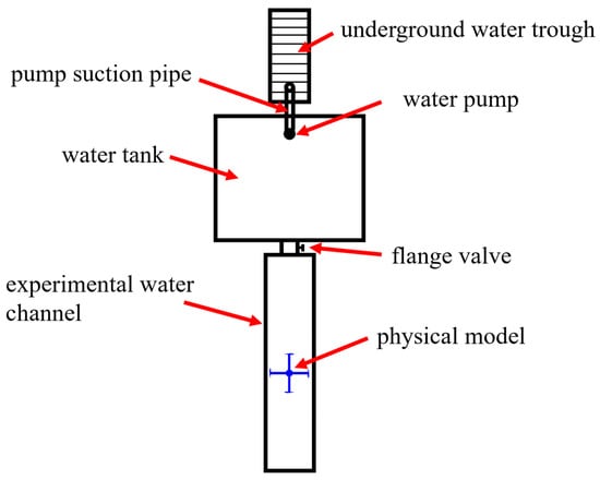
Figure 5. Schematic Diagram of the Experimental Setup.

2.4.2. Measurement System and Uncertainty

Flow velocity was measured using an acoustic Doppler velocimeter (ADV), model HY.LS10-1A, as shown in Figure 6. To capture the undisturbed incoming flow velocity, a velocity measurement cross-section was established 1.5 m upstream of the rotor, consistent with the location of the velocity inlet in the numerical simulation. The cross-section measurement employed a single-point method, with three vertical lines distributed across the section. The ADV probe was positioned on the vertical lines at a distance of 0.6 h from the water surface, where h is the water depth. Two measurements were taken at each point, and the cross-sectional average velocity was calculated from these readings. For each test condition, continuous wave sampling was performed at a frequency of 5000 kHz for 60 s, and the time-averaged value was recorded as the reference velocity.

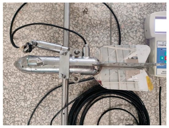
Figure 6. Photograph of the Flow Velocity Measurement Instrument.

Rotational speed was monitored by a rotational speed sensor, model JLBU-1-100KG. The data acquisition system recorded the speed at a frequency of 20 Hz, as shown in Figure 7.

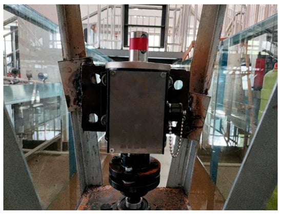
Figure 7. Photograph of the Rotational Speed Measurement Instrument.

Regarding the uncertainty of flow velocity measurement, it includes instrument error and positional error. Based on the manufacturer’s specifications, the instrument error is 0.5%. The positional error accounts for a potential placement error of up to 5 mm for the probe on the vertical lines of the measurement cross-section. For rotational speed measurement, based on the manufacturer’s specifications, the instrument error is 0.5%.

2.4.3. Validation Conditions and Objectives

This experiment validates the accuracy of the 3D CFD model in predicting turbine performance. The validation object is the turbine using the NACA 2414 airfoil. Under different Reynolds numbers induced by adjusting the flow velocity, the prototype was allowed to rotate passively until reaching a stable phase, and the steady-state rotational speed was measured. This yielded curves of the tip speed ratio (TSR) versus Reynolds number, serving as the primary indicator for verifying the reliability of the CFD through experiments.

The experimental TSR values (TSR_exp) for three different Reynolds numbers were calculated and compared with the CFD-predicted values (TSR_CFD). The relative error ε was used to quantify the agreement between simulation and experiment, given by the formula:

$$\epsilon ={\displaystyle \frac{\left|TS{R}_{\exp }-TS{R}_{CFD}\right|}{TS{R}_{CFD}}}\times 100\%$$

(13)

If the relative error is less than the specified threshold of 5%, the validation is considered successful. This proves that the numerical model can accurately capture the hydrodynamic characteristics of the turbine, thereby strongly supporting the conclusions drawn from the screening based on this model.

2.5. Experimental Design Based on RSM

The airfoil is a key component affecting the operational performance of the vertical-axis tidal current turbine. Changes in parameters such as the airfoil’s maximum thickness, location of maximum thickness, and maximum camber will all lead to variations in the turbine’s performance.

The power coefficient (C_P) of the vertical-axis tidal current turbine is influenced by the interactions among multiple parameters. For the key aerodynamic parameters of the airfoil, their value ranges were defined. A high-order Response Surface Methodology (RSM) model was established within these ranges to determine the optimal parameter combination. Three factors were selected: Maximum Thickness (A), Location of Maximum Thickness (B), and Maximum Camber (C). Their specific high and low levels are shown in Table 5.

Table 5. Parameter Range Values.

Level	Factor A (%)	Factor B (%)	Factor C (%)
−1	8	30	0
0	16	45	2
1	24	60	4

A Box–Behnken Design (BBD) was implemented for the three key factors within their predefined ranges. Seventeen experimental runs were conducted, including five center points and twelve edge midpoints. The spatial configuration of the experimental points is shown in Figure 8, and the design matrix is presented in Table 6.

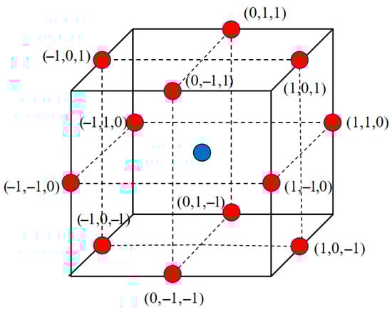
Figure 8. Three-dimensional spatial configuration of the three-factor BBD.

Table 6. Design Matrix.

Airfoil ID	Factor A (%)	Factor B (%)	Factor C (%)
1	24	60	2
2	16	45	2
3	24	45	0
4	16	45	2
5	16	45	2
6	8	30	2
7	16	45	2
8	16	45	2
9	8	45	4
10	8	45	0
11	16	60	4
12	24	45	4
13	8	60	2
14	16	30	0
15	16	60	0
16	16	30	4
17	24	30	2

This design strategy (12 edge midpoints + 5 center points) resulted in a total of 17 unique geometric parameter combinations. For each parameter set, a numerical experiment was conducted using the aforementioned 3D CFD model to obtain its power coefficient (C_P) as the response value. This design efficiently provides all the data necessary for fitting a complete second-order polynomial model with the minimum number of experiments, while ensuring the statistical robustness of the model.

3. Results and Discussion

3.1. Analysis of Experimental Results

Three-dimensional numerical simulations and validation experiments were conducted on a turbine employing the NACA 2414 airfoil under various Reynolds numbers. The average angular velocity over five cycles during the stable operation phase was obtained, from which TSR_CFD and TSR_exp were calculated. Curves depicting their variation with Reynolds number were plotted, as detailed in Figure 9.

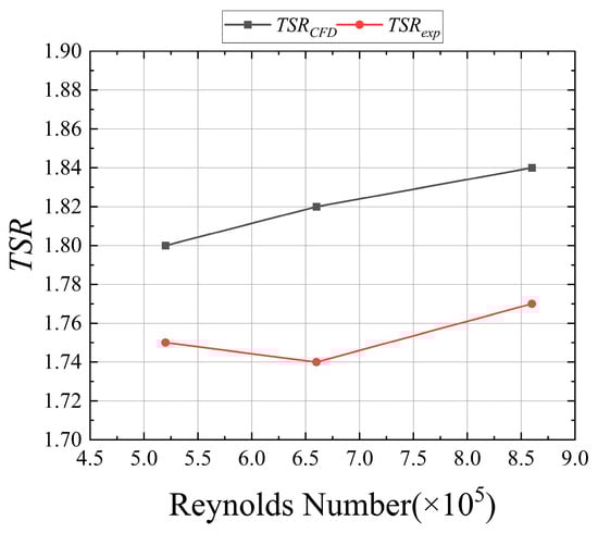
Figure 9. Variation in TSR with Reynolds Number.

Three specific Reynolds number points and their corresponding TSR_CFD and TSR_exp values were selected. The relative error ε was calculated using the error formula, with detailed results presented in Table 7.

Table 7. Comparison of CFD Predictions and Experimental Values for TSR at Different Reynolds Numbers.

Reynolds Number (×105)	TSRCFD	TSRexp	ε
5.2	1.80	1.75	2.6%
6.6	1.82	1.74	4.5%
8.6	1.84	1.77	4.0%

Based on the comparison between 3D CFD simulations and experimental data, within the Reynolds number range of Reynolds number = 5.2 × 10⁵ to 8.6 × 10⁵, the simulated and measured Tip Speed Ratio (TSR) values show good agreement. The maximum relative error is only 4.5%, indicating that the established numerical model can reliably capture the hydrodynamic characteristics of the turbine under different flow velocities. The observed systematic deviation primarily stems from simplifications in the turbulence model, mesh discretization errors, and uncertainties in experimental measurements. However, these minor discrepancies are within the acceptable range for engineering applications.

Through high-precision validation of TSR, this study confirms the reliability of the CFD model for performance comparison. Consequently, the conclusion that the performance of the optimized airfoil is significantly improved, derived from the same model, is credible. This provides a solid verification foundation for the entire parametric optimization process.

3.2. Experimental Results Based on RSM

The power coefficient (C_P) for each design combination in the BBD matrix was obtained through three-dimensional numerical simulations, as shown in Table 8.

Table 8. Calculation Results for Each Design Combination.

Airfoil ID	CP
1	0.1080
2	0.1136
3	0.1194
4	0.1136
5	0.1136
6	0.0752
7	0.1136
8	0.1136
9	0.0348
10	0.0325
11	0.0577
12	0.1453
13	0.0208
14	0.1501
15	0.0159
16	0.1722
17	0.1725

A second-order response surface model was employed to analyze the nonlinear effects of multiple factors on the response variables. The generalized second-order polynomial model takes the form:

$$y={\beta }_0+{\displaystyle \sum _{i=1}^k{\beta }_i}{x}_i+{\displaystyle \sum _{i=1}^k{\beta }_{ii}}{x}_i^2+{\displaystyle \sum _{i<j}{\beta }_{ij}}{x}_i{x}_j+\iota$$

(14)

where y denotes the response variable; x_i, x_j represent the coded independent variables; β₀ is the constant term; β_i signifies the linear effect coefficients; β_ii indicates the quadratic effect coefficients; β_ij corresponds to the interaction effect coefficients; and ι designates the random error.

The experimental datasets were substituted into Equation to fit regression equations for the response variables, establishing relationships between the independent variables x and responses y. The resulting fitted regression equation for C_P is given by Equation (15).

$$\begin{array}{l}{C}_{P_0}=-0.05621+0.01504\times A-0.00235\times B+0.00535\times C\\ -0.00002\times AB+0.00037\times AC+0.00017\times BC\\ -0.00028\times A^2-0.00001\times B^2-0.00322\times C^2\end{array}$$

(15)

Residual plots were used to validate the regression equations. As shown in Figure 10, the samples are significantly and randomly distributed on both sides of the x-axis, indicating the acceptability of the response function. However, relying solely on residual inspection is insufficient to fully assess the goodness of fit of the response surface model, as it may not reveal all potential issues. Therefore, the R-criterion was supplemented for a comprehensive evaluation of the model’s performance and applicability.

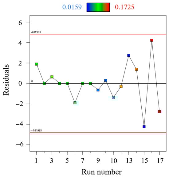
Figure 10. Residual Plot for C_P.

The regression equation was examined using R-squared analysis, and the results are presented in Table 9.

Table 9. Significance Analysis of Regression Equations.

Objective Function	Sum of Squares	Mean Square	F-Value	p-Value	R2	R2adj
CP	0.0386	0.0043	13.15	0.0013	0.9441	0.8723

As shown in Table 9, the p-value for C_P is 0.0013, which is far below the significance threshold (α = 0.05). Simultaneously, the coefficient of determination (R²) is 0.9441, and the adjusted R² (R²_adj) is 0.8723. Integrating these findings with the residual plot analysis indicates that the established model possesses good reliability and robustness.

3.3. Variable Analysis

3.3.1. Main Effects Analysis of Variables

Figure 11 illustrates the regulatory trends of the three key airfoil parameters—Maximum Thickness (A), Location of Maximum Thickness (B), and Maximum Camber (C)—on the power coefficient C_P, with the other two parameters held at their median values. As Maximum Thickness (A) increases, C_P shows a significantly rising positive correlation. In contrast, as the Location of Maximum Thickness (B) increases, C_P continuously decreases, indicating a negative correlation. For Maximum Camber (C), C_P rapidly increases when C rises from 0 to 2, but then slowly declines when exceeding 2, exhibiting an overall characteristic of “rising first, then stabilizing and decreasing.” These differential trends intuitively reflect the directional influence of airfoil geometric parameters on energy extraction efficiency, providing guidance for parameter adjustment in airfoil optimization.

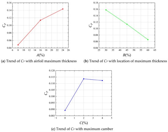
Figure 11. Main effects of the three variables.

3.3.2. Analysis of Interaction Effects Among Variables

Figure 12 reveals the combined influence of pairwise interactions among airfoil parameters on the power coefficient C_P. In the A-B interaction, C_P climbs significantly into a high-value region when A increases and B decreases (thickness located forward), highlighting that their opposing synergy has the most prominent effect on enhancing C_P. In the A-C interaction, an increase in A can maintain C_P in a relatively high range, while changes in C have a gentler impact on C_P, indicating the dominant role of A on C_P. In the B-C interaction, C_P is higher when B decreases and C is within a moderate range, and deviating from this combination leads to a decrease in C_P, though the magnitude of influence is weaker than interactions involving A. Overall, the optimal synergistic direction for improving C_P is “increasing A, positioning B forward, and maintaining C at a moderate level.”

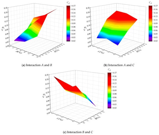
Figure 12. Interaction effects among the three variables.

3.4. Results Analysis

Design-Expert 13 software was used to predict the optimal parameter combination for the rotor. The solution process yielded a total of 100 non-dominated solutions (Pareto solution set) that satisfied the constraints. To determine the global optimal design, the following screening procedure was implemented: (1) First, solutions where design variables were at extreme values were excluded based on engineering manufacturability. (2) Subsequently, from the remaining solutions, 5 candidate points with the highest predicted C_P were selected; their design variables are listed in Table 10. (3) To overcome the prediction uncertainty of the surrogate model, independent, high-precision 3D CFD verification simulations were conducted for these 5 candidate points. A comparison between the simulated and predicted values is shown in Table 11, with errors generally within 5%, demonstrating the reliability of the response surface model. The verification simulations used the same meshing and turbulence models as the response surface construction phase. (4) The verification results (Table 11 and Table 12) show that Optimized Foil 5 achieved a C_P of 0.1887, which is higher than the other candidate points and the original NACA 2414 baseline airfoil (C_P = 0.1480). This indicates that this point lies within a high-performance region where the response surface model fits well.

Table 10. Comparison of Design Parameters between the Baseline and Optimized Pumps.

Airfoil ID	Factor A (%)	Factor B (%)	Factor C (%)
NACA 2414	14.00	30.00	2.00
Optimized Foil 1	23.14	30.12	2.17
Optimized Foil 2	23.79	30.43	2.08
Optimized Foil 3	23.99	31.05	2.28
Optimized Foil 4	22.36	30.20	3.03
Optimized Foil 5	23.51	30.14	3.99

Table 11. Comparison between 3D Numerical Simulation and Response Surface Prediction.

Airfoil ID	Predicted CP	Simulated CP	Error
Optimized Foil 1	0.1891	0.1797	5.2%
Optimized Foil 2	0.1891	0.1818	4.0%
Optimized Foil 3	0.1887	0.1792	5.3%
Optimized Foil 4	0.1884	0.1788	5.3%
Optimized Foil 5	0.1882	0.1887	0.2%

Table 12. Performance Comparison of Turbines with Baseline and Optimized Airfoils.

Airfoil ID	CP	CP Increase	CP Increase Percentage
NACA 2414	0.1480	0.0407	27.5%
Optimized Foil 5	0.1887

The above results demonstrate that the research framework established in this paper—comprising parametric design, response surface optimization, and high-fidelity verification—is highly effective and reliable. The engineering screening of hundreds of Pareto solutions and the direct CFD verification of the 5 candidate points not only ensured the robustness of the optimal solution but also confirmed the good predictive capability of the response surface model within the core design space (prediction error < 5.3%). The finally determined optimized airfoil (Optimized Foil 5), while keeping the location of maximum thickness largely unchanged, significantly increased both thickness and camber. Its power coefficient C_P reached 0.1887, representing a substantial 27.5% improvement over the baseline NACA 2414 airfoil. This significant performance enhancement fully proves that systematic multi-parameter collaborative optimization can effectively overcome the performance bottlenecks of traditional airfoils under low flow velocity conditions, providing a new and effective approach for the blade design of vertical-axis tidal current turbines.

3.5. Research Limitations and Future Work

This study established an effective framework integrating parametric design, response surface optimization, and high-precision validation, successfully enhancing the power coefficient of the vertical-axis tidal current turbine. However, any research has its boundaries and potential for expansion. This section aims to objectively examine the limitations of the current work and propose possible future research directions accordingly.

3.5.1. Research Limitations

The limitations of this study primarily lie in three aspects: model simplification, design space, and validation scope.

Firstly, both the numerical simulations and experimental validation were based on uniform and stable inflow conditions. In reality, tidal currents in actual marine environments are characterized by unsteadiness, high turbulence intensity, and multidirectional variability. The steady turbulence model and uniform velocity inlet settings adopted in this study, while ensuring the controllability and repeatability of fundamental research, may not fully reflect the performance of the optimized airfoil under complex real sea conditions. Secondly, although the variables involved in the parametric optimization—maximum thickness, location of maximum thickness, and maximum camber—are core aerodynamic parameters, they fail to encompass more detailed geometric features such as leading-edge radius and trailing-edge shape. Consequently, the defined design space may not represent the complete space containing the global optimum. Finally, experimental validation was conducted only within a limited operational range of Reynolds numbers from 5.2 × 10⁵ to 8.6 × 10⁵, primarily comparing the key indicator of Tip Speed Ratio (TSR). The performance and robustness of the optimized airfoil under broader flow velocities, tip speed ratios (especially during low-speed start-up conditions), and varying turbulence intensities require further investigation.

3.5.2. Future Work

Based on the aforementioned limitations, future research can be deepened and expanded from the following three levels.

At the level of mechanism and modeling, future studies could employ higher-fidelity turbulence models such as Scale-Adaptive Simulation (SAS) or Large Eddy Simulation (LES), within Fluent 2024 R1, combined with advanced flow field measurement techniques like Particle Image Velocimetry (PIV). This approach would enable a more detailed revelation of the physical essence of how the optimized airfoil controls flow separation and utilizes vortex dynamics. At the level of optimization design, research can evolve towards multi-objective and high-dimensional development. On one hand, considerations for blade load, cavitation characteristics, and noise levels could be incorporated into the optimization objectives to achieve the co-design of performance and reliability. On the other hand, more flexible geometric parameterization methods could be introduced to expand the design space and explore innovative high-performance airfoils that break traditional paradigms. At the level of engineering validation, the final and most critical step is to test the optimized design in real or quasi-real environments. This includes conducting model experiments in circulating water channels simulating shear flows and oscillatory flows under complex conditions, and ultimately advancing to the fabrication of functional prototypes for long-term operational validation in controlled offshore test sites. This would complete the full cycle from numerical optimization to engineering application, providing more practical solutions for the blade design of vertical-axis tidal current turbines.

4. Conclusions

This study conducted an optimal design for the airfoil of a vertical-axis tidal current turbine through a systematic framework integrating parametric design, Computational Fluid Dynamics (CFD) simulation, and experimental validation. The main conclusions are as follows:

(1)

A reliable simulation and optimization design system was established: A three-dimensional CFD model validated by experiments was constructed. Within the Reynolds number range of 5.2 × 10⁵ to 8.6 × 10⁵, the maximum relative error between its predicted Tip Speed Ratio (TSR) and the experimental values was only 4.5%, demonstrating that this model can accurately capture the hydrodynamic characteristics of the turbine, thereby laying a reliable foundation for performance evaluation and optimization.

(2)

The influence patterns of key airfoil parameters were clarified: Analysis based on Response Surface Methodology (RSM) revealed that the maximum thickness (A), the location of maximum thickness (B), and the maximum camber (C) have significant nonlinear effects and interactions on the power coefficient (C_P). The optimal synergistic direction for enhancing turbine performance is increasing the maximum thickness, moving the location of maximum thickness forward, and maintaining the camber at a moderate level.

(3)

A significant performance improvement of the turbine was achieved: Through multi-parameter collaborative optimization, an optimal set of airfoil parameters was obtained. Verification shows that the power coefficient (C_P) of this optimized airfoil reaches 0.1887, representing a substantial increase of 27.5% compared to the baseline NACA 2414 airfoil. This effectively overcomes the performance bottleneck of traditional airfoils under low flow velocity conditions.

(4)

The effectiveness and robustness of the proposed methodological framework were verified: High-precision CFD verification of the optimization results showed errors ranging from 0.2% to 5.3%, indicating the good predictive capability of the established response surface model. The integrated “Parametric Design-Response Surface Optimization–High-Fidelity Verification” framework adopted in this research provides an efficient and reliable new approach for the blade design of vertical-axis tidal current turbines.

References

- Shen, C.Y.; Han, Y.B.; Wang, S.M.; Wang, Z.K. Influence of Airfoil Curvature and Blade Angle on Vertical Axis Hydraulic Turbine Performance in Low Flow Conditions. Water 2025, 17, 11. [Google Scholar] [CrossRef]
- Noorollahi, Y.; Ganji, M.J.Z.; Rezaei, M.; Tahani, M. Analysis of turbulent flow on tidal stream turbine by RANS and BEM. Comput. Model. Eng. Sci. 2021, 127, 515–532. [Google Scholar] [CrossRef]
- Wei, X.S.; Huang, B.; Liu, P.; Kanemoto, T.; Wang, L.Q. Experimental investigation into the effects of blade pitch angle and axial distance on the performance of a counter-rotating tidal turbine. Ocean Eng. 2015, 110, 78–88. [Google Scholar] [CrossRef]
- Huang, B.; Usui, Y.; Takaki, K.; Kanemoto, T. Optimization of blade setting angles of a counterrotating type horizontal-axis tidal turbine using response surface methodology and experimental validation. Int. J. Energy Res. 2016, 40, 610–617. [Google Scholar] [CrossRef]
- Huang, B.; Nakanishi, Y.; Kanemoto, T. Numerical and experimental analysis of a counter-rotating type horizontal-axis tidal turbine. J. Mech. Sci. Technol. 2016, 30, 499–505. [Google Scholar] [CrossRef]
- Huang, B.; Zhu, G.J.; Kanemoto, T. Design and performance enhancement of a bi-directional counter-rotating type horizontal axis tidal turbine. Ocean Eng. 2016, 128, 116–123. [Google Scholar] [CrossRef]
- Huang, B.; Kanemoto, T. Performance and internal flow of a counter-rotating type tidal stream turbine. J. Therm. Sci. 2015, 24, 410–416. [Google Scholar] [CrossRef]
- Gonabadi, H.; Oila, A.; Yadav, A.; Bull, S. Fatigue life prediction of composite tidal turbine blades. Ocean Eng. 2022, 260, 111903. [Google Scholar] [CrossRef]
- Xu, J.; Wang, L.Y.; Yuan, J.P.; Wang, Z.L.; Zhang, B.W.; Luo, Z.H.; Tan, A.C.C. TurbineNet: Advancing tidal turbine blade hydrodynamic performance prediction with neural networks. Phys. Fluids 2025, 37, 027143. [Google Scholar] [CrossRef]
- Huang, B.; Zhao, B.W.; Wang, L.; Wang, P.Z.; Zhao, H.Y.; Guo, P.C.; Yang, S.; Wu, D.Z. The effects of heave motion on the performance of a floating counter-rotating type tidal turbine under wave-current interaction. Energy Convers. Manag. 2022, 252, 115093. [Google Scholar] [CrossRef]
- Liu, X.D.; Xu, H.Y.; Wang, B.H.; Wang, Y.K.; Li, C.L.; Si, Y.L.; Qian, P.; Zhang, D.H. An analytical double-Gaussian wake model of ducted horizontal-axis tidal turbine. Phys. Fluids 2023, 35, 043103. [Google Scholar]
- Mcnaughton, J.; Ettema, S.; Arcos, F.Z.; Vogel, C.R.; Willden, R.H.J. An experimental investigation of the influence of inter-turbine spacing on the loads and performance of a co-planar tidal turbine fence. J. Fluids Struct. 2023, 118, 103844. [Google Scholar] [CrossRef]
- Suhri, G.E.; Rahman, A.A.; Dass, L.; Rajendran, K.; Rahman, A.A. Interactions between tidal turbine wakes: Numerical study for shallow water application. J. Phys. Conf. Ser. 2022, 84, 91–101. [Google Scholar] [CrossRef]
- Wu, Y.N.; Wu, H.; Kang, H.S.; Li, H. Layout optimization of a tidal current turbine array based on quantum discrete particle swarm algorithm. J. Mar. Sci. Eng. 2023, 11, 1994. [Google Scholar] [CrossRef]
- Moreau, M.; German, G.; Maurice, G.; Richard, A. Sea states influence on the behaviour of a bottom mounted full-scale twin vertical axis tidal turbine. Ocean Eng. 2022, 265, 112582. [Google Scholar] [CrossRef]
- Chen, L.; Wang, H.; Yao, Y.; Sun, Z.K.; Chin, R.J. An experimental and numerical assessment of tidal stream turbine behavior under seabed bathymetry proximity and blockage ratio effect. Renew. Energy 2025, 243, 122487. [Google Scholar] [CrossRef]
- Chen, L.; Wang, H.; Yao, Y.; Zhang, Y.Q.; Li, J.X. Experimental investigation of the seabed topography effects on tidal stream turbine behavior and wake characteristics. Ocean Eng. 2023, 281, 114682. [Google Scholar] [CrossRef]
- Gao, Y.J.; Liu, H.W.; Lin, Y.G.; Gu, Y.J.; Ni, Y.M. Hydrodynamic analysis of tidal current turbine under water-sediment conditions. J. Mar. Sci. Eng. 2022, 10, 515. [Google Scholar] [CrossRef]
- Lin, X.F.; Zhang, J.S.; Guan, D.W.; Zheng, J.H.; Zhang, Y.Q.; Rodriguez, E.F.; Gao, L.C. Scour processes around a horizontal axial tidal stream turbine supported by the tripod foundation. Ocean Eng. 2024, 296, 116891. [Google Scholar] [CrossRef]
- Zhang, Y.D.; Shek, J.K.H.; Mueller, M.A. Controller design for a tidal turbine array, considering both power and loads aspects. Renew. Energy 2023, 216, 119063. [Google Scholar] [CrossRef]
- Wang, S.Q.; Tang, J.; Li, C.Y.; Ji, R.W.; Rodriguez, E.F. Performance evaluation and fast prediction of a pitched horizontal-axis tidal turbine under wave-current conditions using a variable-speed control strategy. J. Fluids Struct. 2025, 133, 104265. [Google Scholar] [CrossRef]
- Liu, B.H.; Park, S. Effect of Wavelength on turbine performances and vortical wake flows for various submersion depths. J. Mar. Sci. Eng. 2024, 12, 560. [Google Scholar] [CrossRef]
- Linant, R.; Saouli, Y.; Germain, G.; Maurice, G. Experimental study of the wave effects on a ducted twin vertical axis tidal turbine wake development. J. Mar. Sci. Eng. 2025, 13, 375. [Google Scholar] [CrossRef]
- Xu, J.H.; Zhang, Y.Q.; Zheng, Y.; Gu, Y.J.; Rodriguez, E.F. Investigation of the hydrodynamics and wake characteristics of a floating twin-rotor tidal stream turbine under surge motion with free surface consideration. Energy 2025, 320, 135134. [Google Scholar] [CrossRef]
- Jia, G.T.; Chen, C.; Wang, L.; Wang, P.Z.; Huang, B.; Wu, R. Unsteady hydrodynamic characteristics control of turbine blades by the vortex generators. Ocean Eng. 2025, 324, 120785. [Google Scholar] [CrossRef]
- Heo, M.W.; Ko, D.H.; Park, J.S.; Yi, J.H. Power performance evaluation of a 1 MW tidal current energy converter system installed at Uldolmok Strait. J. Mech. Sci. Technol. 2025, 39, 1625–1634. [Google Scholar] [CrossRef]
- Xu, J.; Wang, L.Y.; Yuan, J.P.; Luo, Z.H.; Wang, Z.L.; Zhang, B.W.; Tan, A.C.C. DLFSI: A deep learning static fluid-structure interaction model for hydrodynamic-structural optimization of composite tidal turbine blade. Renew. Energy 2024, 224, 120179. [Google Scholar] [CrossRef]
- Wei, X.S.; Huang, B.; Kanemoto, T.; Wang, L.Q. Near wake study of counter-rotating horizontal axis tidal turbines based on PIV measurements in a wind tunnel. J. Mar. Sci. Technol. 2017, 22, 11–24. [Google Scholar] [CrossRef]
- Novo, P.G.; Inubuse, M.; Matsuno, T.; Kyozuka, Y.; Archer, P.; Matsuo, H.; Henzan, K.; Sakaguchi, D. Characterization of the wake generated downstream of a MW-scale tidal turbine in Naru Strait, Japan, based on vessel-mounted ADCP data. Energy 2024, 299, 131453. [Google Scholar] [CrossRef]
- Liu, X.D.; Lu, J.K.; Ren, T.S.; Yu, F.; Cen, Y.H.; Li, C.M. Review of research on wake characteristics in horizontal-axis tidal turbines. Ocean Eng. 2024, 312, 119159. [Google Scholar] [CrossRef]
- Maduka, M.; Li, C.W. Experimental evaluation of power performance and wake characteristics of twin flanged duct turbines in tandem under bi-directional tidal flows. Renew. Energy 2022, 199, 1543–1567. [Google Scholar] [CrossRef]
Disclaimer/Publisher’s Note: The statements, opinions and data contained in all publications are solely those of the individual author(s) and contributor(s) and not of MDPI and/or the editor(s). MDPI and/or the editor(s) disclaim responsibility for any injury to people or property resulting from any ideas, methods, instructions or products referred to in the content. |
© 2025 by the authors. Licensee MDPI, Basel, Switzerland. This article is an open access article distributed under the terms and conditions of the Creative Commons Attribution (CC BY) license.