Abstract
With the rapid growth of global shipping, accurate vessel traffic prediction is essential for waterway management and navigation safety. This study proposes the Fusion Spatio-Temporal Transformer (FSTformer) to address non-Gaussianity, non-stationarity, and spatiotemporal heterogeneity in traffic flow prediction. FSTformer incorporates a Weibull–Gaussian Transformation for distribution normalization, a hybrid Transformer encoder with Heterogeneous Mixture-of-Experts (HMoE) to model complex dependencies, and a Kernel MSE loss function to enhance robustness. Experiments on AIS data from the Fujiangsha waters of the Yangtze River show that FSTformer consistently outperforms baseline models across multiple horizons. Compared with the best baseline (STEAformer), it reduces MAE, RMSE, and MAPE by 3.9%, 1.8%, and 6.3%, respectively. These results demonstrate that FSTformer significantly improves prediction accuracy and stability, offering reliable technical support for intelligent shipping and traffic scheduling in complex waterways.
1. Introduction
Nowadays, the shipping industry is experiencing rapid growth and has become the most important mode of global transportation, leading to a significant increase in Vessel Traffic Flow (VTF). Vessel traffic systems are facing mounting operational pressures and safety challenges due to the continuous rise in shipping density. To achieve the efficient allocation of waterway resources, enhance port operational efficiency, and ensure navigational safety, the accurate prediction of VTF has gradually emerged as a key research topic in Intelligent Traffic Systems (ITS). Particularly in complex inland waterways and regions with dense port clusters, the timely perception and prediction of traffic conditions are fundamental to realizing smart shipping, supporting decision-making, and mitigating risks.
As a type of time series data, early research on VTF prediction primarily relied on statistical time series models, such as ARIMA and VAR [1,2]. However, these models are based on the assumption of linearity and address the problem through predefined mathematical formulations.
To capture the nonlinear characteristics of VTF data, some researchers have adopted machine learning models, such as Support Vector Regression (SVR) and Extreme Learning Machine (ELM) [3,4]. Although these models outperform traditional statistical methods, they demand extensive feature engineering efforts. To overcome these limitations, deep learning models have attracted widespread attention in the field of VTF prediction. Their powerful end-to-end learning capabilities enable the automatic extraction of nonlinear features directly from raw data [5,6]. Nonetheless, achieving highly accurate long-term VTF predictions remains a formidable challenge.
Firstly, VTF data exhibit significant spatiotemporal heterogeneity; that is, the VTF shows significant distributional differences across different waterway nodes, as well as fluctuating traffic patterns over different time periods at the same node. As shown in Figure 1a, significant differences are observed in the flow variation trends among multiple waterway nodes during the same time period. Each node exhibits high spatial heterogeneity in terms of peak and valley times, fluctuation amplitudes, and overall patterns of change. Figure 1b further illustrates the change process of a typical node across different time periods; it can be observed that the traffic flow pattern exhibits pronounced periodic fluctuations and asynchronous behavior, reflecting non-stationarity and dynamic variation in the temporal dimension. As a deep learning framework that can model the spatiotemporal heterogeneity of traffic flow, Spatio-Temporal Graph Neural Networks (STGNNs) have attracted widespread attention in recent years, and a large number of scholars have carried out relevant research in this field [7,8]. Nevertheless, most of STGNNs still rely on the static predefined graph structures, implicitly assuming that the spatial relationships between waterway nodes remain fixed through the prediction process. But the connection strength of each node in the traffic network is dynamically changing. This static assumption limits the model’s ability to model the spatial topological relationship in the traffic network, which also limits the prediction performance to a certain extent.
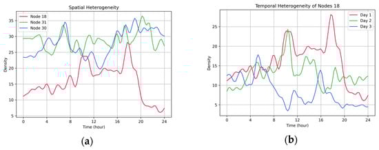
Figure 1.
The spatio-temporal heterogeneity of vessel traffic flow prediction, illustrated using AIS records from the Fujiangsha waterways of the Yangtze River. (a,b) illustrate the spatial and temporal heterogeneity of vessel traffic flow data, respectively.
Secondly, VTF data exhibit both non-stationary and non-Gaussian characteristics. On the one hand, VTF data demonstrate a strong non-stationarity. As illustrated in Figure 2a, the sliding mean and standard deviation of the node continue to fluctuate in multiple time periods, indicating that its time series characteristics change significantly over time and show non-stationary characteristics. On the other hand, VTF data does not strictly follow the Gaussian distribution. As shown in Figure 1b, the probability density function of traffic flow is severely skewed and has a long tail, which indicates that the VTF data presents non-Gaussianity. Such non-stationary and non-Gaussianity challenge traditional modeling approaches, constraining the accuracy and robustness of long-term predictions. Although some researchers have employed sequence decomposition to generate more stable subsequences, these methods still fail to effectively address the underlying non-Gaussianity properties [9,10,11].

Figure 2.
Illustration of non-stationarity and non-Gaussianity of vessel traffic flow, based on AIS data from the Fujiangsha waterways of the Yangtze River. (a) shows the rolling mean and rolling variance of the traffic flow time series of node 18, which shows a trend of fluctuation over time, indicating that the traffic flow has obvious non-stationary characteristics; (b) shows the probability density distribution of the traffic flow at this node, which has skewness and long tail compared to the standard normal distribution, reflecting that its distribution characteristics are non-Gaussian.
Thus, in order to create a dynamic model of the spatiotemporal heterogeneity in vessel traffic network and eliminate its non-stability and non-Gaussianity characteristics as far as possible, we propose a novel model for ship traffic flow prediction, named Fusion Spatio-Temporal Transformer (FSTformer). In light of the non-Gaussianity commonly observed in VTF data, we introduce the Weibull–Gaussian Transform (WGT) at the input stage to Gaussianize the input data, thereby reducing data volatility and enhancing modeling stability [12]. This choice is motivated by the heavy-tailed and skewed nature of raw vessel traffic flow statistics, for which Weibull-based modeling provides a more natural fit compared to conventional transformations. To capture the spatiotemporal heterogeneity of VTF data, we design a fusion spatiotemporal Transformer encoder that integrates Heterogeneous Mixture-of-Experts (HMoE). Specifically, the encoder dynamically incorporates evolving graph structure information into the spatial attention mechanism and introduces a HMoE module consisting of Multilayer Perceptron (MLP) and Temporal Convolutional Network (TCN) components, thus improving the model’s capability to capture complex spatiotemporal dependencies. Moreover, considering that the traditional Mean Squared Error (MSE) loss is susceptible to outliers and can lead to error accumulation in multi-step prediction tasks, we introduce the Kernel MSE loss function. By incorporating kernel-based mappings into the error computation, this method effectively suppresses the influence of large-error samples during gradient updates, thereby enhancing the model’s robustness to outliers and improving the stability and accuracy of long-term predictions. Kernel-based error modeling has been proven effective in mitigating noise sensitivity and improving model generalization in complex environments, such as in wind speed prediction tasks [13].
The main contributions of this paper are summarized as follows:
- A VTF prediction model, Fusion Spatio-Temporal Transformer (FSTformer), is proposed, integrating distribution transformation, spatiotemporal attention modeling, and an expert structure enhancement mechanism. This model effectively adapts to the non-Gaussianity, non-stationarity, and spatiotemporal heterogeneity inherent in VTF data, and demonstrates excellent accuracy and robustness in multi-step prediction tasks.
- The Weibull–Gaussian Transform (WGT) is introduced to map VTF data into a near-Gaussian distribution, reducing data volatility and enhancing model stability and performance.
- A Fusion Spatio-Temporal Transfomer Encoder layer is designed, which embeds dynamic graph structure information into the spatial attention mechanism and incorporates a Heterogeneous Mixture-of-Experts (HMoE) module composed of MLP and TCN components, thereby enhancing the capability to capture complex spatiotemporal heterogeneity within traffic networks.
- The Kernel MSE loss function is employed to improve long-term prediction performance, providing greater robustness to outliers and enhancing the stability of model training, which leads to more accurate multi-step VTF forecasting.
The structure of this paper is as follows: Section 2 reviews related work, including the development of VTF prediction. Section 3 presents the basic framework of the proposed model. Section 4 describes the experimental setup and provides an analysis of the experimental results. Section 5 concludes the paper with a detailed summary of the work.
2. Related Work
VTF prediction is a fundamental problem in Intelligent Transportation Systems and has become a research hotspot with widespread attention in recent years. Early studies primarily relied on time series analysis techniques, such as ARIMA and VAR [2,14]. Experiments have shown that such models struggle to capture the nonlinear features in the data. With the advancement of computer technology, machine learning models, such as ELM and SVR, have been gradually applied in this field [3,15]. In comparison with statistical models, these methods can capture complex nonlinear patterns but demand considerable feature engineering to attain high predictive accuracy.
In recent years, deep learning technology has advanced rapidly and has played a significant role in the field of VTF prediction. RNN and CNN are two fundamental architectures of deep neural networks, each demonstrating unique advantages in VTF prediction tasks. On the one hand, RNNs are well suited for processing time series data. Their variants, such as LSTM [16] and GRU [17], demonstrate strong performance in sequence modeling tasks and have been widely applied in VTF prediction [18,19]. On the other hand, although CNN was originally developed for image processing [20,21], one-dimensional CNN (1D-CNN) can extract local temporal features from continuous windows by sliding along the time axis. The Temporal Convolutional Network (TCN) is a CNN-based architecture designed for temporal processing and has demonstrated excellent performance [22]. It learns multi-scale temporal features by stacking dilated causal convolutions TCN has been widely applied in the field of VTF prediction. For example, the Temporal-TimesNet model proposed by Zhang et al. combines TCN with a time embedding mechanism to achieve multi-step prediction of VTF [23]. In another study, Li and Wang introduced an adaptive genetic algorithm to optimize the TCN structure, effectively improving the accuracy and stability of the predictions [24]. However, neither single RNN models nor CNN models fully consider the spatial relationships within the traffic network. Some studies have shown that CNNs can capture certain spatial dependencies in multi-segment traffic flows through weight sharing. As a result, CNN-RNN-based models have been applied to multi-segment VTF prediction [25,26,27]. This approach achieves a certain degree of separation between spatial and temporal feature modeling. However, due to the irregular distribution of nodes in transportation networks, conventional CNNs remain insufficient for extracting spatial relationships, particularly in non-Euclidean spaces where it is challenging for CNNs to accurately characterize the topological relationships between different nodes.
To address this issue, researchers have introduced graph neural networks (GNNs) to accommodate the irregular spatial structures of transportation networks [28]. GNNs can directly model the relationships between nodes within a graph structure and flexibly capture spatial dependencies by aggregating information from neighboring nodes, thus gradually becoming the mainstream approach for modeling spatial relationships in transportation networks. As types of GNNs, GCN [29] and GAE [30] have achieved promising results in VTF prediction. However, GNNs are less effective than traditional RNN and CNN models in modeling temporal dynamics. Therefore, the combined model of GNNs and temporal models, known as the Spatio-Temporal Graph Neural Networks (STGNNs), have become a research hotspot for spatio-temporal modeling of traffic networks. Based on the type of temporal modeling employed, STGNNs can be broadly categorized into two groups: RNN-based STGNNs and CNN-based STGNNs.
RNN-based STGNNs integrate GNNs with RNN architectures, where representative works such as PG-STGNN [31], MRA-BGCN [32], and ST-MGCN [33] utilize LSTM models to capture temporal features along the time axis. CNN-based STGNNs integrate GNNs with CNN models, such as MSSTGNN [34], STSGCN [35], and STMGCN [36]. By introducing convolutional operations into the graph network, these models efficiently extract traffic patterns within local time windows. Compared to RNN-based structures, CNNs offer stronger parallel computing capabilities and higher training efficiency, demonstrating superior stability particularly when handling short-term temporal dependencies and large-scale datasets.
However, most existing STGNN models are built on the assumption of a static graph structure, which is evidently unrealistic. VTF exhibits pronounced spatiotemporal heterogeneity, and a static network structure prevents the model from capturing dynamic features, thereby limiting its predictive performance. Therefore, neural networks based on dynamic graph structures have emerged as a research hotspot. The Graph Attention Network (GAT) introduces an attention mechanism into graph structures, enabling the capture of dynamic changes in graph topology to a certain extent [37]. Such models have achieved notable success in the transportation domain [38,39,40]. For instance, Li et al. integrated GAT with extended causal convolution to capture traffic patterns that dynamically evolve across spatial and temporal dimensions [38]. Guo et al. proposed ASTGCN, in which the spatiotemporal attention mechanism effectively captures dynamic spatiotemporal correlations [39]. Although GAT introduces an attention mechanism into graph neural networks, allowing adaptive weighting of neighboring nodes and thereby enhancing the modeling of local spatial dynamic relationships, its attention is primarily confined to the spatial neighborhood within the graph structure, making it difficult to capture global temporal dependencies in long time series.
In contrast, the Transformer [41], based on the self-attention mechanism, possesses global modeling capabilities and can significantly improve accuracy in long-term predictions. Li Le et al. combined STGNN with the Transformer architecture and proposed SDSTGNN to perform long-term VTF prediction [42]. Guo et al. developed ASTGNN, which enhances the modeling capabilities of traffic networks by integrating dynamic graph convolutions into the Transformer framework [43]. STGormer incorporated spatiotemporal graph encoding into the self-attention mechanism and introduced a Mixture-of-Experts (MoE) module based on MLPs to capture spatio-temporal heterogeneity in the data [44]. These studies demonstrate that integrating graph structures with Transformer architectures can effectively improve the performance of spatio-temporal modeling. Nevertheless, although these studies show the potential of integrating graph structures with Transformer architectures, they still fall short in fully capturing heterogeneous patterns, handling non-Gaussian data, and ensuring robustness in long-horizon forecasting.
In summary, although existing research has made considerable progress in VTF prediction—particularly through STGNNs and graph-Transformer models that have significantly enhanced the ability to capture complex dependencies—several limitations remain. First, the non-Gaussian characteristics of VTF are generally overlooked, adversely affecting model training stability and generalization capability. Second, there is a lack of deep modeling of dynamic spatial structures and spatiotemporal heterogeneity, making it difficult for models to adapt to drastic changes in traffic patterns across different regions and time periods. Third, limited robustness to outliers hinders the ability to maintain stable performance in multi-step prediction tasks.
To address these challenges, this paper proposes a hybrid spatio-temporal prediction model, Fusion Spatio-Temporal Transformer (FSTformer), which integrates a distribution transformation mechanism, a graph structure enhancement module, and a Heterogeneous Mixture-of-Experts (HMoE) modeling strategy. The model aims to improve stability, flexibility, and robustness at the distribution, structural, and loss function levels, thereby enabling more effective handling of multi-source uncertainties and complex evolution patterns in VTF.
3. Methodology
3.1. Problem Definition
Definition 1.
Traffic Network. In this study, the target area is divided into sub-areas, each of which is treated as a waterway node within the traffic network. The entire traffic network can be represented as , where denoted the set of waterway nodes, represents the set of edges defining the graph structure, and is the adjacency matrix encoding the connections between nodes.
Definition 2.
VTF data. The VTF prediction task aims to forecast future traffic status based on historical traffic information. Accordingly, two categories of data are involved in this task. The first category is the historical traffic status information, represented as , where is the number of nodes, is the historical observation step, and is the number of features. The second category is the feature traffic status information to be predicted, denoted as , where P is the future step to be predicted.
Definition 3.
Prediction Problem. The VTF prediction problem can be formulated as follows: given a traffic network , the goal is to construct a prediction model that utilizes historical traffic status information to forecast future traffic status information . This problem can be mathematically expressed by the following equation:
3.2. Weibull–Gaussian Transform
Weibull–Gaussian Transform (WGT) is a preprocessing method proposed by Brown et al. [45]. In the VTF prediction task, the raw VTF data exhibit strong non-stationary and non-Gaussianity. If used the raw data without preprocessing, the prediction results are likely to exhibit large errors. Thus, we introduce the WGT to eliminate the non-Gaussianity and improve the stability of data. The core idea of WGT is to map the raw data to a Gaussian distribution through the Weibull distribution. The probability density function (PDF) of the Weibull distribution is defined as
where is the origin value, is the shape parameter of Weibull distribution, and is the scale parameter. To transform the VTF data into a Gaussian distribution, WGT first applies a power transformation to the original sequence to obtain the processed sequence , which is given by
where is the transformed data, which follows a Weibull distribution with the shape parameter . Dubey et al. demonstrated that when the shape parameter approaches 3.6, the Weibull distribution can be approximated by a Gaussian distribution [46].
Then, the transformed data should be standardized to further enhance the stationarity as follows:
where and denote the expectation and variance operations, represents the time series after processing.
3.3. FSTformer
To model the spatio-temporal heterogeneity, a deep learning model named FSTformer is proposed. FSTformer is a neural network based on the Transformer architecture and consists of a Spatio-Temporal Position Embedding layer, a Fusion Spatio-Temporal Transfomer Encoder layer and an Output layer, as illustrated in Figure 3. Each encoder layer comprises two core feature extraction modules: the Fusion Spatio-Temporal Attention Mechanism and the Heterogeneous Mixture-of-Experts (HMoE). This section provides a detailed introduction to the proposed model.
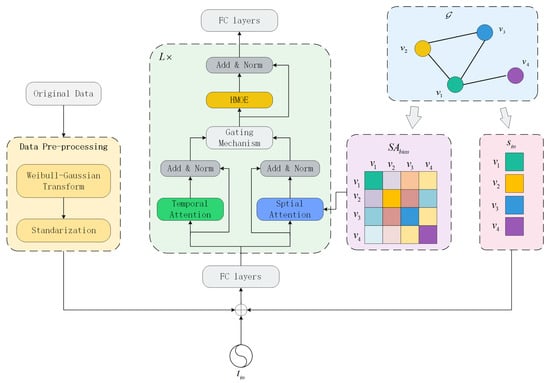
Figure 3.
The structure of FSTformer.
3.3.1. Spatio-Temporal Position Embedding Layer
Since FSTformer does not incorporate any RNN structures, it is necessary to embed positional information into the data to help the model better capture the structure of the time series. This is achieved through two embedding strategies: Temporal Position Encoding and Spatial Position Encoding.
For temporal embedding, we use the sine and cosine formula commonly used in the Transformer model, which is:
where is the relative index of the data in the sequence, represents the embedding dimension of the model, and refers to the dimension of the position encoding vector.
For the spatial embedding, we use the degree centrality of nodes in the graph structure. Degree centrality reflects the importance of a node within the overall graph. In the context of a ship traffic network, nodes with higher degrees are more likely to serve as transportation hubs and thus play a more critical role in the network. Specifically, the spatial position encoding based on degree centrality is calculated as follows:
where and represent the in-degree and out-degree of the traffic node respectively, while and are learnable parameters for the spatial embedding.
Finally, the input data is added with the temporal embedding and spatial embedding , as illustrated below:
where represent the data after spatial and temporal embedding, is the Fully Connected layer.
3.3.2. Fusion Spatio-Temporal Attention Mechanism
To capture the spatiotemporal features in the VTF network, attention mechanisms are applied separately along the temporal and spatial axes, followed by a gating mechanism to fuse the extracted features.
The self-attention mechanism serves as the core feature extraction module in the Transformer architecture, enabling the model to capture dynamic global dependencies. Along the temporal dimension, we employ the multi-head self-attention mechanism to model the temporal characteristics of the data. Given an input feature sequence after position embedding , we first project it into the query, key, and value spaces via linear transformations:
where , , are the learnable projection matrices. Then, the temporal characteristics can be calculated by the following equation:
where denotes the temporal attention weights, represents the embedding dimension.
Along the spatial dimension, we adjust the multi-head attention mechanism by incorporating the shortest path distance (SPD) between each pair of nodes in the graph structure as prior information to calculate the spatial attention weights. In our model, the underlying graph topology based on the SPD is fixed and used as a prior. However, the effective graph structure is dynamically updated through the spatial attention mechanism: at each training step, the attention weights are re-computed based on the evolving node features and temporal context, which results in time-varying edge weights. Thus, while the topological connectivity remains static, the functional adjacency matrix is dynamic and adaptive to traffic conditions. This approach has been validated in previous studies, such as in [44,47]. Therefore, the formula for computing the spatial attention weights and the spatial characteristics is as follows:
where represents the graph structure of the vessel traffic network, is an elementwise learnable scalar shared across all spatial attention layers.
Finally, we use a gating mechanism to fuse the temporal and spatial features, which is defined as follows:
where represents the fused spatio-temporal characteristics, and the gating parameter is a trainable weight that adaptively controls the fusion of spatial and temporal features. It allows the model to dynamically adjust their relative contributions during training, ensuring more flexible and stable spatio-temporal representation learning.
3.3.3. Heterogeneous Mixture-of-Experts
To model the diverse patterns and heterogeneous features in VTF data, we replace the traditional feedforward neural network (FFN) layer in the Transformer architecture with a Heterogeneous Mixture-of-Experts (HMoE) module. There are two types of experts in the HMoE module, namely the Multi-Layer Perceptron (MLP) and the Temporal Convolutional Network (TCN), which focus on static structural feature extraction and temporal dynamic modeling, respectively.
MLP is a fundamental and efficient feedforward neural network structure, primarily composed of multiple linear transformation layers and nonlinear activation functions (e.g., ReLU). In the HMoE module, the MLP subnetwork is mainly employed to model static structural feature in the input features. The formulation is as follows:
where and represent the weight matrix and bias vector of the i-th fully connected layer, respectively.
TCN can extract dynamic features over a large temporal receptive field while preserving temporal order through the use of causal and dilated convolutions. In this model, TCN experts are employed to capture the dynamic temporal characteristics. The formula of TCN is as follows:
where indicates the current time step, is the dilation rate controlling the spacing between kernel elements, represents the learnable weight associated with the i-th convolution position, is the kernel size, and denotes the convolutional operation.
To enable dynamic expert selection, we design a lightweight gated routing network that receives the fused spatio-temporal features and outputs an E-dimensional softmax distribution , where E is the total number of experts, with half being MLPs and half TCNs. Each dimension corresponds to the selection probability of an expert. The formula to calculate the distribution is as follows:
where refers to either a TCN or an MLP expert.
Finally, the weighted fusion of all experts’ outputs can be expressed as follows:
where and represent the i-th gated routing network and expert, respectively.
In this study, we used a multi-layer perceptron (MLP) and a temporal convolutional network (TCN) to construct the HMoE because they offer complementary advantages in modeling VTF. On the one hand, the MLP is a simple and efficient feedforward neural network and is also the core component of the FFN layer in the standard Transformer. It can capture static structural patterns in sequences by increasing and decreasing dimensionality. On the other hand, the TCN, through its dilated causal convolutional architecture, can extract long-range dependencies and capture dynamic changes in sequences. This architecture has been widely used in dynamic time series modeling [22,23,24]. While other architectures (such as RNNs or CNNs) could also be used, our design choice was based on a balance between effectiveness, computational efficiency, and consistency with the overall Transformer framework.
3.3.4. Output Layer
At the end of the model, a fully connected layer is used to map the high-dimensional features to the predicted VTF values, as follows:
where denotes the predicted VTF value, and represent the weight matrix and bias vector of the fully connected layer, respectively.
3.4. Loss Function
The Mean Squared Error (MSE) loss function is commonly used in time series prediction models. However, it typically evaluates the discrepancy between the predicted and true values in a linear feature space, which presents certain limitations for VTF data with strong nonlinear characteristics. To better capture the nonlinearity in prediction errors, a kernel-based MSE loss function is introduced. By mapping the errors into a high-dimensional kernel space, this approach enhances the model’s ability to fit complex patterns.
The kernel loss function maps the predicted values and true values from the original space into a kernel space through a mapping function . In the kernel space, the Euclidean distance between any two points can be calculated using a Mercer kernel, as illustrated below:
Using the kernel function, the squared distance in the kernel space can be expressed as:
where represent represents the inner product in the kernel space, and is the square of distance in kernel space.
Thus, the Kernel MSE loss function can be formulated as:
In this study, we set . Compared to the MSE loss function, the Kernel MSE loss function offers the following advantages:
- Its first-order derivative remains positive, thereby maintaining a gradient direction similar to that of the MSE loss function.
- Its second-order derivative is negative, indicating that as the error increases, the growth rate of the loss slows down, thereby reducing the impact of outliers on the training process.
- Compared with the traditional MSE loss function, the Kernel MSE loss function better preserves the details of small errors and exhibits greater robustness to large errors.
To prevent the gating network from over-relying on a few experts, we introduce a load balancing loss to encourage a more balanced utilization of all experts. Defining the average activation ratio of each expert as , the load balancing loss is formulated as follows:
where is the total number of the expert.
In summary, the total loss function of the model is defined as
4. Experiment
In this section, we conduct detailed experiments on the proposed model to demonstrate the excellent performance of FSTformer in the VTF prediction task. First, this section introduces the data used in the experiment in detail and explains the necessity and effect of using WGT. Secondly, the comparison model and the evaluation indicators used in this experiment are introduced. Finally, FSTformer and the comparison model are compared on real datasets and the differences are analyzed. In addition, in order to verify the effects of each improved module in FSTformer, relevant ablation experiments are also conducted and analyzed.
4.1. Data Description
The data used in this experiment are derived from AIS records collected in the Fujiangsha waterways of the Yangtze River, China. Based on the geographic layout and feasible navigation directions of the waterways in the Fujiangsha region, we divided the area into 41 waterway nodes to construct a waterway traffic network. The divided traffic network and its topological structure are illustrated in Figure 4.
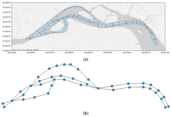
Figure 4.
The location of Fujiangsha waterways and the corresponding waterway graph structure. (a) shows the water division in the study area and the geographical location of each node. (b) shows the graph structure network constructed based on the waterway division, where the nodes represent the segments and the edges represent the connectivity between the segments, which is used to model the flow characteristics of ships in the waterway system.
The original AIS data span from 1 May 2021 to 31 October 2021. We calculated the vessel traffic density at each waterway node at 15 min intervals. Vessel traffic density is defined as the number of vessels per square kilometer at a node at a given time, expressed in units of vessels/km−2.
Before training, the original AIS data were carefully preprocessed to ensure the data quality and the model stability. First, we used the Interquartile Range (IQR) method to identify and correct abnormal data, which effectively mitigated the influence of extreme noise. Then, the Savitzky–Golay (SG) filter was applied to smooth short-term fluctuations while retaining the underlying traffic trends [48]. Next, we used the WGT method to map VTF data into a near-Gaussian distribution. Finally, following Liu et al. [49], we transformed the smoothed data into a recurrent-style structure for time series prediction.
Figure 5 shows the distribution statistics of the vessel traffic density data at the selected nodes using probability density functions and Q-Q plots, respectively. It can be seen from the figure that the traffic density data at these nodes deviate significantly from the Gaussian distribution. Specifically, the histograms show varying degrees of skewness and long-tail behavior, indicating that they have non-Gaussianity. The corresponding Q-Q plots further confirm this observation, with the empirical quantiles deviating from the theoretical Gaussian line, especially at the tail of the distribution. These results highlight the complexity and heterogeneity of ship traffic patterns, and the need to deal with such complex traffic patterns in order to obtain more accurate traffic flow prediction results.
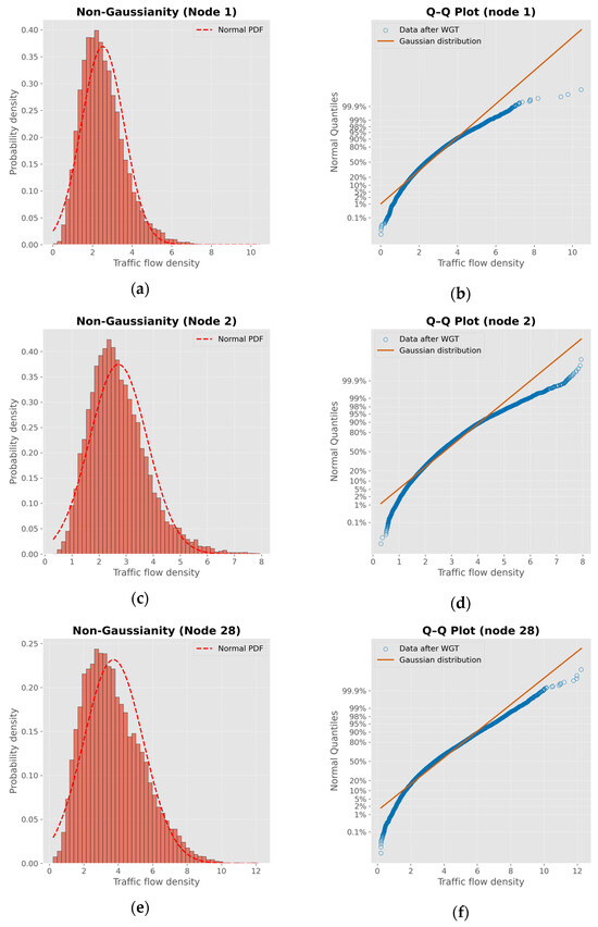
Figure 5.
Non-Gaussianity analysis of vessel traffic flow density at some nodes. (a,c,e) show the probability density histograms of the traffic flow density of nodes 1, 2 and 28, all of which deviate significantly from the normal distribution (red dotted line); (b,d,f) are the Q-Q diagrams of the corresponding nodes. There is a significant deviation between the real data and the theoretical Gaussian distribution, which further verifies that the ship traffic flow exhibits non-Gaussian characteristics in different areas.
We evaluate the normality of the data using the Shapiro–Wilk test (W statistic) along with two additional statistical measures: skewness and kurtosis. The formulas for these three methods are given below:
where is the i-th sample value after sort, represents the mean value of the sample, and n is the sample size. The null hypothesis () of the test states that the data follow a normal distribution, while the alternative hypothesis () indicates that the data do not follow a normal distribution. The calculated p-value is compared with a significance level. If the p-value is less than 0.05, we reject the null hypothesis and conclude that the data do not follow a normal distribution. Conversely, if the p-value is greater than or equal to 0.05, we fail to reject the null hypothesis, suggesting that the data follow a normal distribution.
where n is the sample size, represents the mean value of the sample, and s denotes the standard deviation of the sample. Skewness measures the symmetry of a distribution. For an ideal normal distribution, the skewness value should be zero. A positive skewness (Skewness > 0) indicates that the distribution is right-skewed (with a longer right tail), while a negative skewness (Skewness < 0) indicates that the distribution is left-skewed (with a longer left tail). The absolute magnitude of the skewness value reflects the degree of asymmetry in the distribution.
Kurtosis quantifies the sharpness of a distribution relative to a normal distribution. Under the Fisher definition, a standard normal distribution has zero kurtosis. Positive kurtosis indicates heavier tails and a sharper peak, while negative kurtosis indicates lighter tails and a flatter distribution. Higher kurtosis values are associated with a greater probability of extreme values.
We use the Weibull–Gaussian Transform (WGT) method to preprocess the original data, with the aim of improving the model’s ability to model non-Gaussian data. Table 1 presents the comparative results of the vessel traffic density data before and after the WGT, while Figure 6 illustrates the distribution characteristics using Q-Q plots. It can be observed that before the transformation, the p-values of the density data are generally low, and both skewness and kurtosis are relatively high, indicating pronounced non-Gaussian characteristics. After applying WGT, although the p-values remain below 0.05, they increase significantly, and both skewness and kurtosis decrease. These results suggest that, compared to the original data, the WGT-transformed data more closely approximates a Gaussian distribution.

Table 1.
Normality test and statistical comparison of traffic flow distribution before and after WGT transformation.
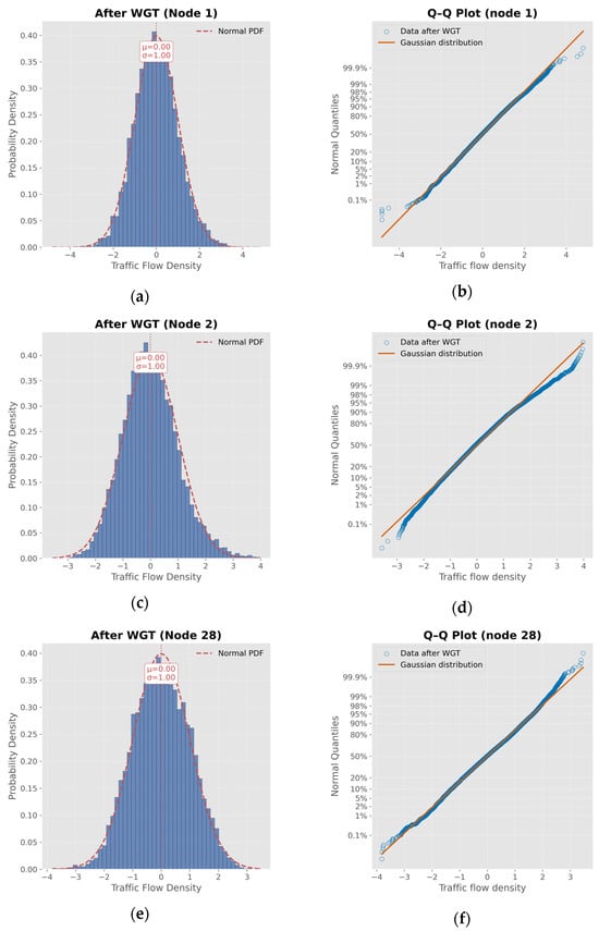
Figure 6.
Gaussian enhancement of vessel traffic flow density after WGT transformation. (a,c,e) show the probability density distribution of traffic flow density at nodes 1, 2, and 28 after applying WGT (Warped Gaussian Transformation), which are highly consistent with the standard normal distribution (red dashed line); (b,d,f) are Q-Q diagrams of the corresponding nodes, showing that the consistency between the data distribution and the Gaussian distribution is significantly enhanced, indicating that WGT effectively improves the Gaussianity of traffic flow data.
4.2. Comparative Model
We selected four categories of models for a comparative study on vessel traffic flow prediction, representing a progression from shallow to deep spatio-temporal integration. Time series models (LSTM, GRU) focus on temporal dynamics; graph network models (GCN, T-GCN) incorporate spatial dependencies; spatio-temporal graph networks (STGNN, STSGCN) jointly model space and time; and spatio-temporal Transformers (STGormer, STAEformer) capture complex long-range dependencies via self-attention. This systematic comparison aims to reveal the relative strengths and weaknesses of each approach to inform model selection and optimization. The detailed introduction to each model is provided below.
- LSTM: The Long Short-Term Memory (LSTM) network, a variant of the Recurrent Neural Network (RNN), retains information through a gating mechanism comprising forget, input, and output gates. The output gate regulates the information used for predicting future time steps.
- GRU: The Gated Recurrent Unit (GRU) is a variant of the LSTM network that simplifies the architecture by combining the forget gate and the input gate into a single update gate.
- GCN: The Graph Convolutional Network (GCN) is a graph neural network model that captures spatial dependencies between nodes through graph convolution operations.
- T-GCN: The Temporal Graph Convolutional Network (T-GCN) extends GCN by integrating time series modeling capabilities, enabling simultaneous spatial and temporal feature extraction.
- STGNN: The Spatio-Temporal Graph Neural Network (STGNN) combines graph convolution and time series models to capture both spatial topological structures and temporal dynamics, making it suitable for prediction tasks involving spatiotemporal coupling characteristics.
- STSGCN: The Spatio-Temporal Synchronous Graph Convolutional Network (STSGCN) proposes a novel convolutional operation that simultaneously captures temporal and spatial correlations.
- STAEformer: The Spatio-Temporal AutoEncoder Transformer (STAEformer) integrates the Transformer self-attention mechanism with an autoencoder architecture, enabling efficient extraction of deep features and long-range dependencies from spatiotemporal data.
- STGormer: The Spatio-Temporal Graph Transformer (STGormer) embeds attribute gating and MoE modules into the multi-head self-attention mechanism, enhancing the model’s ability to capture complex spatiotemporal heterogeneity in vessel traffic data.
4.3. Experiment Setting
We divide the dataset into training, validation, and test sets with a ratio of 7:1:2. For the prediction task, the model uses data from the past 12 time steps to predict vessel traffic flow for the next 6 time steps. We evaluate model performance using MAE, RMSE, and MAPE, which quantify absolute and relative prediction errors. For all metrics, lower values correspond to better performance. The formula for each evaluation indicator is as follows:
where and represent the true value and the predicted value, respectively.
We conducted the experiments on a server equipped with a Hygon C86 7360 24-core processor CPU (Inspur Information, Jinan, China) and an Nvidia A10 GPU (NVIDIA Corporation, Santa Clara, CA, USA), running Ubuntu 24.04 as the operating system. The programming language used was Python 3.8.20, and the deep learning framework was PyTorch 2.4.1. The model was configured with an embedding dimension of 64, three hybrid spatiotemporal encoder layers, eight attention heads, and six experts, evenly divided between MLP and TCN experts. We used the Adam optimizer with a batch size of 128 and an initial learning rate of 0.001, which decayed during training. To accelerate convergence, we employed an early stopping strategy: if the validation loss did not decrease for 25 consecutive epochs, training was terminated, and the best model parameters were saved.
4.4. Experiment Analysis
To compare the performance of different models across various prediction horizons, we conducted a detailed comparison of each model’s results at steps 1 to 6 in all 41 nodes from the Fujiangsha waterways, as shown in Table 2. To provide an intuitive comparison, Figure 7 presents the predicted vessel traffic flow of different models against the ground truth at representative nodes. It highlights that FSTformer’s predictions are consistently closer to the actual values, especially in medium- and long-term steps, while other models show growing deviations.
Table 2.
Error comparison of different models in multi-step ship traffic flow prediction task.
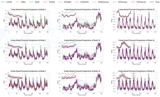
Figure 7.
Comparison between the predicted VTF of different models and the ground truth at representative nodes. The figure highlights that FSTformer maintains closer alignment with actual values, particularly in mid- and long-term predictions, whereas other models show increasing deviations.
In our analysis, predictions at steps 1–2 are defined as short-term predictions, steps 3–4 as mid-term predictions, and steps 5–6 as long-term predictions. The results demonstrate that the proposed FSTformer consistently outperforms other models across all prediction steps, with particularly notable advantages in mid- and long-term forecasting. The RMSE values of FSTformer from the first to the sixth prediction step are 0.317, 0.711, 1.108, 1.359, 1.501, and 1.595, respectively, maintaining the best performance across all models.
Comparison results show that FSTformer maintains consistently lower errors across all forecasting steps, while traditional models (LSTM, GRU, GCN, T-GCN) exhibit rapid error escalation. For instance, the RMSE for LSTM increases from 0.376 to 2.10, GRU from 0.526 to 2.03, and GCN from 2.11 to 2.71, revealing an exponential error growth trend. These findings suggest that traditional models gradually lose temporal modeling capability over longer horizons. FSTformer’s RMSE increased steadily from 0.317 to 1.594 over six steps, with a total rise of only 1.276, much lower than other models. Even at steps 5 and 6, the RMSE remained between 1.5 and 1.6, whereas STAEformer and STGormer exceeded 1.60 and 1.71, respectively. This more than 0.1 gap highlights FSTformer’s superior stability in long-term dependency modeling.
To better illustrate the differences between mathematically predicted values and AIS observations, we summarize the error metrics of FSTformer against baseline models. At the first prediction step, FSTformer already shows the lowest errors (MAE = 0.21, RMSE = 0.32, MAPE = 5.4%), slightly outperforming STAEformer while clearly surpassing GCN. By the third step, its advantage becomes more pronounced, with MAE/RMSE/MAPE of 0.75/1.11/16.1%, compared to 0.80/1.16/16.6% for STAEformer and 1.53/2.32/25.9% for GCN. Even at the sixth step, where errors typically accumulate, FSTformer remains stable (1.08/1.59/21.8%) and outperforms all competitors. On average across all prediction steps, FSTformer achieved errors of 0.74/1.10/15.7% (MAE/RMSE/MAPE), representing relative improvements of 4.2%, 2.0%, and 6.2%, respectively, over the second-best model STAEformer (0.77/1.12/16.7%). Thus, the results demonstrate that FSTformer not only achieves the lowest average errors but also provides consistent and tangible improvements across all evaluation metrics, underscoring its superior reliability for multi-step vessel traffic flow prediction.
Notably, FSTformer exhibits a much lower error growth rate than other models. Between steps 1–3 and 4–6, its RMSE increases by only 0.397 and 0.243, respectively, whereas GCN exceeds 0.59 in the later stages, reflecting rapid error escalation. We further analyzed the RMSE growth slopes, confirming that FSTformer maintains the lowest initial RMSE and achieves stable, controlled error growth. Although STGormer and STAEformer show lower slopes in some intervals, their overall RMSE remains higher and increases sharply in long-term predictions, indicating weaker stability.
This comprehensive performance advantage can be attributed to the multiple optimizations incorporated into the FSTformer model design. The Weibull–Gaussian Transform (WGT) module effectively smooths the non-Gaussian characteristics of vessel traffic flow data during the preprocessing stage, bringing the data distribution closer to a standard normal distribution and enhancing the stability of subsequent modeling. The HMoE structure combines two subnetworks: MLP and TCN. The MLP is adept at extracting spatial static patterns, while the TCN is better suited for capturing temporal dependencies and dynamic trends. The integration of these two types of experts enables the model to simultaneously account for spatial heterogeneity and temporal complexity. Additionally, the introduction of the Kernel MSE loss function suppresses the influence of large error points during the optimization process, thereby enhancing the robustness of the model in long-sequence forecasting tasks and mitigating the error accumulation problem.
In summary, FSTformer not only outperforms all baseline models in terms of average evaluation metrics, but also demonstrates superior stability in multi-step prediction, better adaptability across different tasks, and stronger capability in modeling complex data characteristics. These advantages not only validate the rationality and effectiveness of the model architecture but also provide a feasible technical solution for intelligent vessel traffic management and scheduling in complex waterways.
4.5. Ablation Experiment
In order to further verify the effectiveness of each module in FSTformer, we conducted a detailed ablation experiment. The variant models of the ablation experiment include the following types:
- w/o WGT: In this model, the WGT transformation module is omitted and the commonly used Standard method is used to process the data to verify the impact of non-Gaussian data on the model.
- w/o Kernel MSE: In this model, the Kernel MSE loss function is omitted and replaced with the traditional MSE loss function.
- Full MLP MoE: In this variant, only MLP experts are used within the MoE structure to assess the contribution of TCN experts for time series modeling.
- Full TCN MoE: In this variant, only TCN experts are used within the MoE structure to evaluate the modeling capability of MLP experts for static features.
- w/o MoE: This model replaces the MoE structure with a standard feedforward neural network (FFN) in the Transformer to evaluate the overall effectiveness of the heterogeneous expert structure.
Except for the modifications or removals made to verify the characteristics of specific modules, all variant models follow the same architecture and hyperparameters as FSTformer. Figure 8 presents the results of the ablation experiments on the dataset, including both the average prediction error and the error at different prediction time steps.
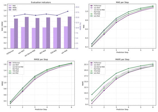
Figure 8.
The results comparison of ablation experiment.
By comparing the performance of the full FSTformer model with the variant without WGT, we observe that removing the WGT data preprocessing module results in a significantly larger prediction error. The average error of the variant without WGT ranks second to last among all models, only outperforming the variant without MoE. These results indicate that processing vessel density data with WGT, by enhancing its Gaussianity, effectively stabilizes the distribution characteristics of the input data and facilitates more effective feature learning by the model.
In addition, the Kernel-based MSE loss function demonstrates better effectiveness compared to the standard MSE loss. Figure 9 presents the loss curves of the Kernel MSE loss and the conventional MSE loss, respectively. It can be observed that the convergence curve of the model using the Kernel MSE loss is more stable, indicating that the kernel method enhances the robustness of the model.
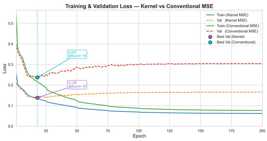
Figure 9.
Comparison of training and validation loss of Kernel MSE and conventional MSE loss functions.
The ablation results further emphasize the importance of the MoE structure. Single-expert variants using only MLP or TCN, as well as models without MoE, show significantly inferior performance compared to the full FSTformer. Notably, the performance gap widens with longer prediction steps, highlighting the necessity of heterogeneous expert modeling for capturing complex long-term temporal dependencies.
4.6. The Sensitivity Analysis of σ in Kernel MSE Loss Function
To further justify the choice of selection in the Kernel MSE loss function, we conducted the sensitivity experiment on different .
Figure 10 illustrates how the kernel bandwidth influences the performance of the model. From the theoretical perspective, controls both the curvature of the loss near zero error and the rate at which the loss saturates for the large errors.
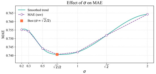
Figure 10.
Effect of the kernel bandwidth on MAE.
A very small (e.g., 0.2–0.3) produces a steep curvature around zero, making the model overly sensitive to noise while quickly suppressing medium and large errors. Conversely, when the becomes large (e.g., 1–2), the loss function behaves increasingly like the standard MSE, where robustness against outliers is weakened and long-horizon error accumulation degrades performance, as reflected by the rising MAE. Between these two extremes, a moderate strikes a balance: at , the MAE reaches its lowest value. This choice ensures that small errors are learned with sufficient precision, while abnormal large deviations are precented from dominating the optimization. These results confirm that provides the most appropriate trade-off between accuracy and robustness, justifying it as the default setting in out experiments.
4.7. Comparison of Gaussianization Functions in Prediction Performance
To further validate the choice of the Weibull-Gaussian Transform (WGT) we selected, we compared the prediction performance of FSTformer with two other Gaussianization transformations (Box–Cox [50] and Yeo–Johnson [51]), as well as a baseline that only applied Standard normalization. Figure 11 reports the multi-step prediction MAE results.
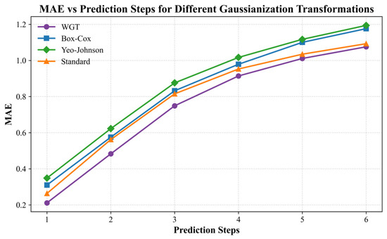
Figure 11.
Comparation of the FSTformer prediction performance on different Gaussianization transformations.
The results show that WGT consistently achieves the lowest errors across all prediction steps. In particular, WGT yields significant improvements at short prediction steps (1–3), and still maintains competitive advantages as the prediction step increases. Although Box–Cox and Yeo–Johnson transformations perform better in statistical Gaussianization tests, their prediction performance lags behind the WGT, even lags to the Standard transformation, suggesting that they cannot optimally preserve the spatio-temporal patterns which are required for robust prediction. These findings demonstrate WGT strikes a favorable balance between distributional regularization and predictive accuracy, supporting its adoption as the primary transformation method in this study.
5. Conclusions
In this paper, we proposed FSTformer, a novel spatio-temporal prediction model specifically designed for vessel traffic flow forecasting. To address the non-Gaussian characteristics commonly observed in vessel traffic data, we employed the Weibull–Gaussian Transform (WGT), which effectively enhances the Gaussianity of input features and improves model stability.
To capture the complex spatio-temporal dependencies inherent in vessel traffic networks, we employed attention mechanisms along both the temporal and spatial dimensions. Furthermore, a gating mechanism was incorporated to adaptively fuse information from temporal and spatial representations, enabling the extraction of more comprehensive dynamic features. We also replaced the traditional feedforward fully connected layer in the Transformer architecture with a Heterogeneous Mixture-of-Experts (HMoE) module. This design allows the model to better capture spatio-temporal heterogeneity across different nodes and time steps, significantly enhancing its representational capacity. Additionally, we adopted a Kernel MSE loss function during training to further improve model robustness. Compared to the conventional MSE loss, the Kernel MSE loss effectively mitigates the influence of outliers and stabilizes the training process, leading to more reliable performance, especially in long-term forecasting tasks.
Extensive experiments on real-world vessel traffic datasets demonstrate the effectiveness of the proposed approach. The results show that FSTformer consistently outperforms existing baseline models in terms of both accuracy and stability, confirming its potential as a powerful tool for intelligent maritime transportation systems.
Despite these promising results, this study has two main limitations: it does not address scenarios with severely corrupted or missing data, and it is validated only on the Fujiangsha waterway datasets. In future work, we will explore incorporating additional multimodal variables (e.g., weather, water level data) and extend validation to more datasets, as well as investigate the practical deployment of FSTformer in real-world traffic management systems. In addition, robust prediction under conditions of missing data will also be an important direction to enhance the applicability of the model in real-world AIS environments.
Author Contributions
Conceptualization, M.P.; methodology, D.Z., S.L., Y.L. and M.P.; software, D.Z. and M.P.; validation, D.Z., H.X. and M.P.; resources, H.X. and M.P.; data curation, Y.G. and Y.L.; writing—original draft preparation, D.Z. and M.P.; writing—review and editing, D.Z., H.X. and M.P.; funding acquisition, M.P. and H.X. All authors have read and agreed to the published version of the manuscript.
Funding
This work was developed by the National Natural Science Foundation of China (NSFC) under grant No. 52371363, the Guangxi Science and Technology Infrastructure and Talent Development Program under grant No. GUIKE AD25069109, and the Fund of State Key Laboratory of Maritime Technology and Safety under grant No. 21-15-1.
Data Availability Statement
The dataset is not publicly available due to confidentiality agreements with the data provider.
Conflicts of Interest
Author Haichao Xu was employed by the company Bvision Intelligent Technology Co., Ltd., Nanjing. The remaining authors declare that the research was conducted in the absence of any commercial or financial relationships that could be construed as a potential conflict of interest.
Abbreviations
The following abbreviations are used in this manuscript:
| FSTformer | Fusion Spatio-Temporal Transformer |
| MoE | Mixture-of-Experts |
| HMoE | Heterogeneous Mixture-of-Experts |
| VTF | Vessel Traffic Flow |
| AIS | Automatic Identification System |
| LSTM | Long Short-Term Memory |
| GRU | Gated Recurrent Unit |
| ITS | Intelligent Traffic Systems |
| ARIMA | Autoregressive Integrated Moving Average |
| ELM | Extreme Learning Machine |
| SVR | Support Vector Regression |
| STGNN | Spatio-Temporal Graph Neural Network |
| TCN | Temporal Convolutional Network |
| MSE | Mean Squared Error |
| WGT | Weibull–Gaussian Transform |
| VAR | Vector Auto-Regression |
| CNN | Convolutional Neural Network |
| RNN | Recurrent Neural Network |
| GNN | Graph Neural Network |
| PG-STGNN | Physics-Guided Spatio-Temporal Graph Neural Network |
| MRA-BGCN | Multi-Range Attentive Bicomponent Graph Convolutional Network |
| ST-MGCN | Spatio-Temporal Multi-Graph Convolution Network |
| MSSTGNN | Multi-Scaled Spatio-Temporal Graph Neural Network |
| STSGCN | Spatial-Temporal Synchronous Graph Convolutional Network |
| STMGCN | Spatio-Temporal Multi-Graph Convolutional Network |
| GAT | Graph Attention Network |
| ASTGNN | Attention-based Spatial-Temporal Graph Neural Network |
| ASTGCN | Attention-Based Spatial-Temporal Graph Convolutional Network |
| SDSTGNN | Semi-Dynamic Spatial–Temporal Graph Neural Network |
| SPD | Shortest Path Distance |
| FFN | Feed-Forward Network |
| MLP | Multi-Layer Perceptron |
| Q-Q plot | Quantile-Quantile Plot |
| STAEformer | Spatio-Temporal Adaptive Embedding Transformer |
| STGormer | Spatio-Temporal Graph Transformer |
| MAE | Mean Absolute Error |
| RMSE | Root Mean Squared Error |
| MAPE | Mean Absolute Percentage Error |
References
- Zhang, G.P. Time series forecasting using a hybrid ARIMA and neural network model. Neurocomputing 2003, 50, 159–175. [Google Scholar] [CrossRef]
- Lu, Z.; Zhou, C.; Wu, J.; Jiang, H.; Cui, S.Y. Integrating granger causality and vector auto-regression for traffic prediction of large-scale WLANs. KSII Trans. Internet Inf. Syst. 2016, 10, 136–151. [Google Scholar]
- Wu, C.H.; Ho, J.M.; Lee, D.T. Travel-time prediction with support vector regression. IEEE Trans. Intell. Transp. Syst. 2004, 5, 276–281. [Google Scholar] [CrossRef]
- Huang, G.B.; Zhu, Q.Y.; Siew, C.K. Extreme learning machine: A new learning scheme of feedforward neural networks. In Proceedings of the 2004 IEEE International Joint Conference on Neural Networks (IEEE Cat. No. 04CH37541), Budapest, Hungary, 25–29 July 2004; IEEE: New York, NY, USA, 2004; Volume 2, pp. 985–990. [Google Scholar]
- Li, Y.; Liang, M.; Li, H.; Yang, Z.L.; Du, L.; Chen, Z.S. Deep learning-powered vessel traffic flow prediction with spatial-temporal attributes and similarity grouping. Eng. Appl. Artif. Intell. 2023, 126, 107012. [Google Scholar] [CrossRef]
- Wang, J.; Wang, X.; Zhou, J. Model selection for predicting marine traffic flow in coastal waterways using deep learning methods. Ocean. Eng. 2025, 329, 121151. [Google Scholar] [CrossRef]
- Yu, B.; Yin, H.; Zhu, Z. Spatio-temporal graph convolutional networks: A deep learning framework for traffic forecasting. arXiv 2017, arXiv:1709.04875. [Google Scholar]
- Zhao, L.; Song, Y.; Zhang, C.; Liu, Y.; Wang, P.; Lin, T.; Deng, M.; Li, H.F. T-GCN: A temporal graph convolutional network for traffic prediction. IEEE Trans. Intell. Transp. Syst. 2019, 21, 3848–3858. [Google Scholar] [CrossRef]
- Wang, D.; Meng, Y.R.; Chen, S.Z.; Xie, C.; Liu, Z. A hybrid model for vessel traffic flow prediction based on wavelet and prophet. J. Mar. Sci. Eng. 2021, 9, 1231. [Google Scholar] [CrossRef]
- Xing, W.; Wang, J.B.; Zhou, K.W.; Li, H.H.; Li, Y.; Yang, Z.L. A hierarchical methodology for vessel traffic flow prediction using Bayesian tensor decomposition and similarity grouping. Ocean Eng. 2023, 286, 115687. [Google Scholar] [CrossRef]
- Huan, Y.; Kang, X.Y.; Zhang, Z.J.; Zhang, Q.; Wang, Y.J.; Wang, Y.F. AIS-based vessel traffic flow prediction using combined EMD-LSTM method. In Proceedings of the 4th International Conference on Advanced Information Science and System, Sanya, China, 25–27 November 2022; pp. 1–8. [Google Scholar]
- Shi, Z.; Li, J.; Jiang, Z.Y.; Li, H.; Yu, C.Q.; Mi, X.W. WGformer: A Weibull-Gaussian Informer based model for wind speed prediction. Eng. Appl. Artif. Intell. 2024, 131, 107891. [Google Scholar] [CrossRef]
- Chen, X.; Yu, R.; Ullah, S.; Wu, D.M.; Li, Z.Q.; Li, Q.L.; Qi, H.G.; Liu, J.H.; Liu, M.; Zhang, Y.D. A novel loss function of deep learning in wind speed forecasting. Energy 2022, 238, 121808. [Google Scholar] [CrossRef]
- Sadeghi Gargari, N.; Akbari, H.; Panahi, R. Forecasting short-term container vessel traffic volume using hybrid ARIMA-NN model. Int. J. Coast. Offshore Environ. Eng. 2019, 4, 47–52. [Google Scholar] [CrossRef]
- Zhang, Q.; Jian, D.; Xu, R.; Dai, W.; Liu, Y. Integrating heterogeneous data sources for traffic flow prediction through extreme learning machine. In Proceedings of the 2017 IEEE International Conference on Big Data (Big Data), Boston, MA, USA, 11–14 December 2017; IEEE: New York, NY, USA, 2017; pp. 4189–4194. [Google Scholar]
- Hochreiter, S.; Schmidhuber, J. Long short-term memory. Neural Comput. 1997, 9, 1735–1780. [Google Scholar] [CrossRef]
- Chung, J.; Gulcehre, C.; Cho, K.H.; Bengio, Y. Empirical evaluation of gated recurrent neural networks on sequence modeling. arXiv 2014, arXiv:1412.3555. [Google Scholar] [CrossRef]
- Ji, Z.; Wang, L.; Zhang, X.; Wang, F. 2022 Ship traffic flow forecast of Qingdao port based on, L.S.T.M. In Proceedings of the Sixth International Conference on Electromechanical Control Technology and Transportation, Chongqing, China, 14–16 May 2021; SPIE: Bellingham, WA, USA, 2021; Volume 12081, pp. 587–595. [Google Scholar]
- Xu, X.; Bai, X.; Xiao, Y.; He, J.; Xu, Y.; Ren, H. A port ship flow prediction model based on the automatic identification system gated recurrent units. J. Mar. Sci. Appl. 2021, 20, 572–580. [Google Scholar] [CrossRef]
- LeCun, Y.; Bottou, L.; Bengio, Y.; Haffner, P. Gradient-based learning applied to document recognition. Proc. IEEE 1998, 86, 2278–2324. [Google Scholar] [CrossRef]
- Krizhevsky, A.; Sutskever, I.; Hinton, G.E. Imagenet classification with deep convolutional neural networks. Adv. Neural Inf. Process. Syst. 2012, 25, 84–90. [Google Scholar] [CrossRef]
- Bai, S.; Kolter, J.Z.; Koltun, V. An empirical evaluation of generic convolutional and recurrent networks for sequence modeling. arXiv 2018, arXiv:1803.01271. [Google Scholar] [CrossRef]
- Zhang, D.; Zhao, L.N.; Liu, Z.Y.; Pan, M.Y.; Li, L. Temporal-TimesNet: A novel hybrid model for vessel traffic flow multi-step prediction. Ships Offshore Struct. 2025, 1–14. [Google Scholar] [CrossRef]
- Li, Y.; Wang, Q. Adaptive genetic algorithm-optimized temporal convolutional networks for high-precision ship traffic flow prediction. Evol. Syst. 2025, 16, 4. [Google Scholar] [CrossRef]
- Wu, Y.Y.; Zhao, L.N.; Yuan, Z.X.; Zhang, C. CNN-GRU ship traffic flow prediction model based on attention mechanism. J. Dalian Marit. Univ. 2023, 49, 75–84. [Google Scholar]
- Chang, Y.; Ma, J.; Sun, L.; Ma, Z.Q.; Zhou, Y. Vessel Traffic Flow Prediction in Port Waterways Based on POA-CNN-BiGRU Model. J. Mar. Sci. Eng. 2024, 12, 2091. [Google Scholar] [CrossRef]
- Narmadha, S.; Vijayakumar, V. Spatio-Temporal vehicle traffic flow prediction using multivariate CNN and LSTM model. Mater. Today Proc. 2023, 81, 826–833. [Google Scholar] [CrossRef]
- Scarselli, F.; Gori, M.; Tsoi, A.C.; Hagenbuchner, M.; Monfardini, G. The graph neural network model. IEEE Trans. Neural Netw. 2008, 20, 61–80. [Google Scholar] [CrossRef]
- Kipf, T.N.; Welling, M. Semi-supervised classification with graph convolutional networks. arXiv 2016, arXiv:1609.02907. [Google Scholar]
- Kipf, T.N.; Welling, M. Variational graph auto-encoders. arXiv 2016, arXiv:1611.07308. [Google Scholar] [CrossRef]
- Pan, Y.A.; Li, F.L.; Li, A.R.; Niu, Z.Q.; Liu, Z. Urban intersection traffic flow prediction: A physics-guided stepwise framework utilizing spatio-temporal graph neural network algorithms. Multimodal Transp. 2025, 4, 100207. [Google Scholar] [CrossRef]
- Chen, W.; Chen, L.; Xie, Y.; Cao, W.; Gao, Y.S.; Feng, X.J. Multi-range attentive bicomponent graph convolutional network for traffic forecasting. In Proceedings of the AAAI Conference on Artificial Intelligence, New York, NY, USA, 7–12 February 2020; Volume 34, pp. 3529–3536. [Google Scholar]
- Geng, X.; Li, Y.G.; Wang, L.Y.; Zhang, L.Y.; Yang, Q.; Ye, J.P.; Liu, Y. Spatiotemporal multi-graph convolution network for ride-hailing demand forecasting. In Proceedings of the AAAI Conference on Artificial Intelligence, Honolulu, HI, USA, 27 January–1 February 2019; Volume 33, pp. 3656–3663. [Google Scholar]
- Qu, Y.; Jia, X.L.; Guo, J.H.; Zhu, H.R.; Wu, W.B. MSSTGNN: Multi-scaled Spatio-temporal graph neural networks for short-and long-term traffic prediction. Knowl.-Based Syst. 2024, 306, 112716. [Google Scholar] [CrossRef]
- Song, C.; Lin, Y.F.; Guo, S.N.; Wan, H.Y. Spatial-temporal synchronous graph convolutional networks: A new framework for spatial-temporal network data forecasting. In Proceedings of the AAAI Conference on Artificial Intelligence, New York, NY, USA, 7–12 February 2020; Volume 34, pp. 914–921. [Google Scholar]
- Liang, M.; Liu, R.W.; Zhan, Y.; Li, H.H.; Zhu, F.H.; Wang, F.Y. Fine-grained vessel traffic flow prediction with a spatio-temporal multigraph convolutional network. IEEE Trans. Intell. Transp. Syst. 2022, 23, 23694–23707. [Google Scholar] [CrossRef]
- Veličković, P.; Cucurull, G.; Casanova, A.; Romero, A.; Li`o, P.; Bengio, Y. Graph attention networks. arXiv 2017, arXiv:1710.10903. [Google Scholar]
- Li, Y.; Li, Z.X.; Mei, Q.; Wang, P.; Hu, W.L.; Wang, Z.S.; Xie, W.X.; Yang, Y.; Chen, Y.R. Research on multi-port ship traffic prediction method based on spatiotemporal graph neural networks. J. Mar. Sci. Eng. 2023, 11, 1379. [Google Scholar] [CrossRef]
- Guo, S.N.; Lin, Y.F.; Feng, N.; Song, C.; Wang, H.Y. Attention based spatial-temporal graph convolutional networks for traffic flow forecasting. In Proceedings of the AAAI Conference on Artificial Intelligence, Honolulu, HI, USA, 27 January–1 February 2019; Volume 33, pp. 922–929. [Google Scholar]
- Wang, Y.; Jing, C.F.; Xu, S.S.; Guo, T. Attention based spatiotemporal graph attention networks for traffic flow forecasting. Inf. Sci. 2022, 607, 869–883. [Google Scholar] [CrossRef]
- Vaswani, A.; Shazeer, N.; Parmar, N.; Uszkoreit, J.; Jones, L.; Gomez, A.N.; Kaiser, Ł.; Polosukhin, I. Attention is all you need. In Advances in Neural Information Processing Systems; MIT Press: Cambridge, MA, USA, 2017; p. 30. [Google Scholar]
- Li, L.; Pan, M.Y.; Liu, Z.Y.; Sun, H.; Zhang, R.L. Semi-dynamic spatial–temporal graph neural network for traffic state prediction in waterways. Ocean Eng. 2024, 293, 116685. [Google Scholar]
- Guo, S.; Lin, Y.F.; Wan, H.Y.; Li, X.C.; Cong, G. Learning dynamics and heterogeneity of spatial-temporal graph data for traffic forecasting. IEEE Trans. Knowl. Data Eng. 2021, 34, 5415–5428. [Google Scholar] [CrossRef]
- Zhou, J.; Liu, E.D.; Chen, W.; Zhang, S.R.; Liang, Y.X. Navigating Spatio-Temporal Heterogeneity: A Graph Transformer Approach for Traffic Forecasting. arXiv 2024, arXiv:2408.10822. [Google Scholar] [CrossRef]
- Brown, B.G.; Katz, R.W.; Murphy, A.H. Time series models to simulate and forecast wind speed and wind power. J. Appl. Meteorol. Climatol. 1984, 23, 1184–1195. [Google Scholar] [CrossRef]
- Dubey, S.Y.D. Normal and Weibull distributions. Nav. Res. Logist. Q. 1967, 14, 69–79. [Google Scholar] [CrossRef]
- Ying, C.; Cai, T.L.; Luo, S.J.; Zheng, S.X.; Ke, G.L.; He, D.; Shen, Y.M.; Liu, T.Y. Do transformers really perform badly for graph representation? Adv. Neural Inf. Process. Syst. 2021, 34, 28877–28888. [Google Scholar]
- Krishnan, S.R.; Seelamantula, C.S. On the selection of optimum Savitzky-Golay filters. IEEE Trans. Signal Process. 2012, 61, 380–391. [Google Scholar] [CrossRef]
- Liu, Z.; Xu, X.H.; Pan, M.Y.; Loo, C.K.; Li, S.X. Weighted error-output recurrent echo kernel state network for multi-step water level prediction. Appl. Soft Comput. 2023, 137, 110131. [Google Scholar] [CrossRef]
- Box, G.E.P.; Cox, D.R. An analysis of transformations. J. R. Stat. Soc. Ser. B Stat. Methodol. 1964, 26, 211–243. [Google Scholar] [CrossRef]
- Yeo, I.K.; Johnson, R.A. A new family of power transformations to improve normality or symmetry. Biometrika 2000, 87, 954–959. [Google Scholar] [CrossRef]
Disclaimer/Publisher’s Note: The statements, opinions and data contained in all publications are solely those of the individual author(s) and contributor(s) and not of MDPI and/or the editor(s). MDPI and/or the editor(s) disclaim responsibility for any injury to people or property resulting from any ideas, methods, instructions or products referred to in the content. |
© 2025 by the authors. Licensee MDPI, Basel, Switzerland. This article is an open access article distributed under the terms and conditions of the Creative Commons Attribution (CC BY) license (https://creativecommons.org/licenses/by/4.0/).