Abstract
To address the issues of external unknown disturbances and roll motion in the tracking control of underactuated unmanned surface vehicle (USV) formation, a cooperative formation control method based on nonlinear model predictive control (NMPC) algorithm and finite-time disturbance observer is proposed. Initially, a tracking error model for the USV formation is established within a leader–follower framework, utilizing a four-degree-of-freedom (4-DOF) dynamic model to simultaneously account for roll motion and trajectory tracking. This error model is then approximately linearized and discretized. To mitigate the initial non-smoothness in the desired trajectories of the follower USVs, a tracking differentiator is designed to smooth the heading angle of the leader USV. Thereafter, a quasi-infinite horizon NMPC algorithm is developed, in which a terminal penalty function is constructed based on quasi-infinite horizon theory. Furthermore, a finite-time disturbance observer is developed to facilitate real-time estimation and compensation for unknown marine disturbances. The proposed method’s effectiveness is validated both mathematically and in simulation. Mathematically, closed-loop stability is rigorously guaranteed via a Lyapunov-based proof of the quasi-infinite horizon NMPC design. In simulations, the algorithm demonstrates superior performance, reducing steady-state tracking errors by over 80% and shortening convergence times by up to 75% compared to a conventional PID controller. These results confirm the method’s robustness and high performance for complex USV formation tasks.
1. Introduction
Unmanned surface vehicles (USVs) have been playing an increasingly important role in a wide range of maritime activities, including marine resource exploration, waterborne rescue, and military operations. Compared to a single USV, multi-USV formations possess greater capability and flexibility for carrying out complex marine tasks and missions [1,2,3]. Cooperative formation control of USVs generally refers to the regulation of USV formations to maintain a prescribed configuration while accurately tracking a desired trajectory, which serves as a fundamental prerequisite for multi-USV systems to accomplish various complex formation-based operations [4,5]. Extensive research has been conducted on this subject, leading to significant advancements in the field.
A novel sliding surface-based distributed control law for USV formation was proposed by Jiang et al. [6], ensuring finite-time convergence. To address parameter uncertainties and complex disturbances, an accurate disturbance observer (ADO) along with a novel fixed-time fast terminal sliding mode (FTFTSM) controller was designed by Shen et al. [7]. For the formation tracking control of USVs under directed graphs, Sui et al. [8] provided a prescribed-time cooperative tracking control scheme, in which a state observer-based prescribed-time sliding surface was developed. A sliding mode observer to obtain the desired trajectory for each USV was developed by Duan et al. [9]. Dong et al. [10] effectively suppressed high-frequency oscillations in the controller caused by complex marine disturbances through the coordinated design of dynamic surface sliding mode control and a lateral velocity tracking differentiator.
A double closed-loop fast integral terminal sliding mode control method was proposed by Xia et al. [11], which not only improved the stability of the leader–follower formation strategy, but also significantly overcame the issue of non-convergence of formation tracking errors within a finite time, commonly observed in traditional approaches. To achieve trajectory tracking control of USV formations with unknown model parameters and environmental disturbances, Dong et al. [12] proposed a data-driven adaptive fuzzy sliding mode control scheme. An online identification algorithm based on navigation data feedback was designed to address the problem of unknown model parameters, thereby enabling real-time acquisition of USV model parameters for the construction of a real-time synchronous formation model. For the underactuated USV formation control problem in environments with static obstacles, model uncertainties, and time-varying disturbances, Huang et al. [13] developed a self-structuring fuzzy Mexican hat wavelet cerebellar model articulation controller based on the Mexican hat wavelet function, thereby achieving model-free control.
The nonlinear model predictive control (NMPC) algorithm achieves control of complex nonlinear systems through online receding-horizon optimization. This approach features advantages such as predictive capability, rolling optimization, and feedback correction [14,15,16]. By incorporating a model predictive mechanism and an online optimization framework, the NMPC algorithm decomposes a complex infinite-horizon optimization problem into finite-horizon subproblems that can be solved in real time. In this manner, an optimal control sequence for the system is generated within each sampling interval. With the rapid advancement of computational capabilities in recent years, the application of NMPC in USV formation control has been increasingly investigated. Zhang et al. [17] proposed a dual closed-loop MPC scheme enhanced by a finite-time extended state observer (ESO) to achieve AUV formation tracking under compound disturbances. A formation tracking error model for USVs was constructed, and a virtual transition trajectory was introduced to guide the design of the tracking controller, particularly to address large initial tracking errors. A dual closed-loop distributed robust MPC algorithm was proposed in [18] to address formation control problems characterized by time-varying communication delays, current disturbances, and model uncertainties.
To address the challenges associated with formation tracking and obstacle avoidance, an event-triggered adaptive NMPC method was developed by Li et al. [19]. Zhu et al. [20] formulated a distributed event-triggered adaptive model predictive control (DEAMPC) approach for formation control, leveraging information from neighboring agents to address trajectory tracking issues in both UAVs and USVs. A distributed formation control strategy for USVs based on NMPC was designed by Liu et al. [21], through which connectivity maintenance and collision avoidance in multi-USV systems were achieved. A path following and collision avoidance system for autonomous surface vehicles based on NMPC was proposed by Gonzalez-Garci et al. [22]. effectively maintained the vehicle’s controlled-speed path tracking, while deviations from the reference trajectory were permitted to safely maneuver around unexpected obstacles.
Based on the analysis of existing research, it has been identified that studies [6,7,8,9,10,11,12,13,14,15,16,17,18,19,20,21] predominantly design control algorithms based on three-degree-of-freedom (3-DOF) models of USVs, with insufficient consideration given to the effects of roll motion on tracking control. In works [6,7,8], cooperative formation control algorithms are developed under the assumption of fully actuated USVs. However, in practical engineering applications, most USVs are underactuated as a result of inherent nonlinear dynamics and actuator limitations. Studies [10,11,12,13,18,19] achieve the generation and maintenance of USV formations based on a leader–follower approach, yet they do not address the pronounced fluctuations in the desired trajectories of follower USVs during the initial tracking phase, which is influenced by the leader’s heading angle. Furthermore, the stability analysis is not provided in [21,22].
Based on the aforementioned analysis, a control approach is presented in this paper, in which a finite-time disturbance observer and a quasi-infinite horizon NMPC algorithm are employed to address the tracking control challenges encountered by underactuated USV formations under marine disturbances and roll motion. Unlike the cited works, which are based on the conventional 3-DOF model (surge, sway, yaw), this study develops its control algorithm based on a 4-DOF model. We explicitly account for and control the USV’s roll motion, which is a significant factor for stability and performance in realistic marine environments. A tracking differentiator is designed to process the heading angle of the leader USV, so that the fluctuations in the desired trajectories of the follower USVs during the initial stage are mitigated. To simultaneously address the roll motion and trajectory tracking control problems of USV formation, a tracking error model is constructed. This model is subsequently subjected to approximate linearization and discretization. A quasi-infinite horizon NMPC algorithm is then proposed, in which a terminal penalty function is designed to ensure the stability of the algorithm. Finally, a finite-time disturbance observer is designed to estimate and compensate for unknown marine disturbances, thereby enhancing the robustness and tracking accuracy of the proposed control scheme.
Compared with existing research, the innovations of this paper are summarized as: (1) The effect of roll motion in underactuated USVs is taken into account, and a trajectory tracking control algorithm is developed based on a 4-DOF mathematical model of the USV. (2) To address the issue of pronounced fluctuations in the desired trajectory of the follower USVs during the initial stage of the tracking task, a tracking differentiator is constructed to smooth the attitude angle of the leader USV, thereby enhancing tracking control performance. (3) A terminal penalty function is designed based on quasi-infinite horizon theory, and terminal inequality constraints are constructed, leading to the development of a quasi-infinite horizon NMPC algorithm. This ensures the stability of the algorithm within the finite prediction horizon. (4) A finite-time disturbance observer is designed and applied to the 4-DOF model of the USV to enable real-time estimation and compensation of unknown marine disturbances.
The remainder of this paper is organized as follows: In Section 2, the USV model and the formation error model are established. In Section 3, a tracking control algorithm for USV formation is designed utilizing the NMPC algorithm in conjunction with a finite-time disturbance observer. Section 4 is dedicated to the stability analysis of the proposed algorithm. In Section 5, the effectiveness and stability of the algorithm are validated through simulation experiments conducted under three different cases.
2. System Model
2.1. Mathematical Model of USV
The development of an accurate mathematical model is fundamental to the design of effective motion control algorithms for USVs. While the majority of research simplifies the control problem by considering only the horizontal motions—specifically, the surge, sway, and yaw degrees of freedom (DOF)—this approach often neglects the critical influence of roll motion.
For USVs operating in realistic wave environments, roll motion is readily excited by wave disturbances and can severely compromise vehicle stability and performance. To enhance the fidelity of our model and the robustness of the subsequent control strategy, this paper incorporates roll dynamics, constructing a comprehensive four-degree-of-freedom (4-DOF) model that captures the coupled motions of surge, sway, roll, and yaw.
According to the literature [23], we consider a formation system comprising N USVs. The kinematic and dynamic equations for the USV are presented. The model accounts for rigid-body dynamics, hydrodynamic effects, and environmental disturbances.
As shown in Figure 1, the kinematic equations describe the geometry of motion, relating the time derivatives of position and orientation in the earth-fixed inertial frame to the linear and angular velocities in the body-fixed frame.
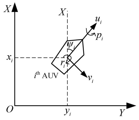
Figure 1.
Diagram of USV Motion.
And the dynamic equations describe the relationship between forces/moments acting on the vehicle and the resulting changes in its linear and angular velocities, following Newtonian and Eulerian mechanics.
where denote the longitudinal and lateral position of the USV. are the roll angle and the yaw angle of the USV, respectively. represent the surge velocity, sway velocity, roll angular velocity, and yaw angular velocity of the USV, respectively. correspond to the hydrodynamic coefficients acting on the four degrees of freedom. denotes the USV’s mass. represent the vertical positions of the center of gravity, the center of buoyancy, and the weight of the USV, respectively. are the control inputs. represent the environmental disturbances acting on the surge, sway, roll, and yaw motions, respectively.
2.2. Formation Tracking Error System
In this paper, a leader–follower scheme is employed to enable the USV formation. The formation is assumed to comprise a single leader USV and follower USVs. The overall structure of the leader–follower framework is depicted in Figure 2.
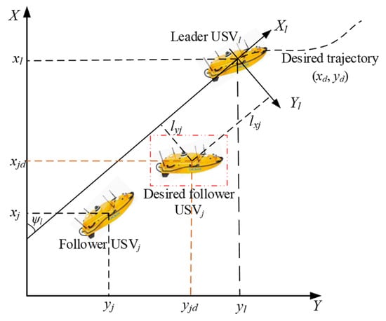
Figure 2.
Leader–follower framework.
As shown in Figure 2, the USV functions as a follower vessel relative to the leader USV. Let denote the position of the leader USV. represent the position of the follower USV, and denote its desired position vector, which can be derived from the leader’s positional information, as detailed below:
where represents the heading angle of the leader, while denotes the relative position of the follower. Specifically, and refer to the desired relative longitudinal and lateral positions, respectively, in the coordinate frame of the leader USV.
Differentiating Equation (2) and combining with Equation (1), we have [24]:
where represent the surge velocity, sway velocity, and yaw angular velocity of the leader USV, respectively.
Considering the drift angle of the follower USV, and in conjunction with Equation (1), we can design the remaining desired state variables for the follower USV as follows:
where are the desired roll angle and heading angle of the USV. represent the desired longitudinal and lateral velocity of the UMV, respectively. denote the desired roll and yaw angular velocity of the UMV, respectively. The method for calculating the desired state variables of the leader USV is consistent with that of the follower USVs.
To facilitate the following discussion, let denotes the desired state vector of the USV and denotes its actual state vector.
The tracking error model is constructed as follows: First, predefined desired positions are used to compute additional desired state variables, which are tracked by the leader USV. The desired states of follower USVs are generated within the leader-follower frame-work. Subsequently, the tracking error model is formulated by subtracting the desired state from the actual state of each USV. The tracking error model translates formation-level goals into individual USV trajectory tracking tasks. Under the leader-follower framework, the leader USV tracks a predefined global trajectory and each follower USV maintains a relative position relative to the leader. Errors are computed relative to time-varying desired states, enabling dynamic formation reconfiguration.
Consequently, the tracking control problem for the USV is transformed into designing an appropriate control input such that the tracking error approaches zero.
3. Control Algorithm Design
This paper addresses the aforementioned control problem using the NMPC algorithm to achieve coordinated tracking control of USV formation under the influence of marine disturbances. The detailed formation control process is illustrated in the flowchart shown in Figure 3.
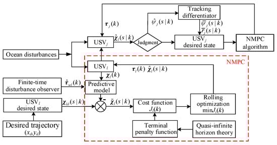
Figure 3.
Flowchart of cooperative formation control.
As shown in Figure 3, the control algorithm design for both the leader USV and the follower USVs is consistent. Therefore, only the design for the USV will be described in detail. Specifically, Section 3.1 outlines the design of a tracking differentiator to smooth the desired trajectory of the USV, Section 3.2 details the design of the NMPC algorithm, and the design of a finite-time disturbance observer is presented in Section 3.3.
3.1. Desired Trajectory Processing
In the context of the NMPC framework, the design of the tracking control algorithm for the USV requires the desired state variables within the prediction horizon . Therefore, this section introduces the assumed state variables of the leader USV within the prediction horizon at time step , as well as the assumed control increments within the control horizon . The details are as follows:
where and represent the assumed control increment sequence and assumed state sequence of the leader USV at time step . and refer to the optimal predicted control increment sequence and optimal state sequence obtained for the leader USV at time step through the NMPC algorithm. denotes the terminal controller of the leader USV at time step , with its specific design detailed in Section 3.2. Finally, represents the terminal state calculated based on the USV model and the terminal controller.
It should be noted that, according to Equation (2), the desired position of the follower USV is highly sensitive to the heading angle of the leader USV. During the initial stages of the tracking task, the discrepancy between the leader’s actual and desired positions is considerable, resulting in significant fluctuations in its actual trajectory. Consequently, the desired trajectory of the follower USV also exhibits pronounced variability.
To mitigate this issue, a tracking differentiator is developed in this section to smooth the leader USV’s heading angle over the prediction horizon at time step . This smoothing process ensures that the resulting desired trajectory for the follower USV is both smooth and well-aligned. The inputs and outputs of the tracking differentiator at time step are illustrated in Figure 4.
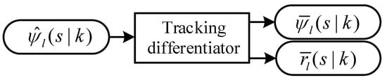
Figure 4.
Tracking differentiator.
In Figure 4, the output signal represents the smoothed hypothetical heading angle of the leader USV, which is used to track the input signal . The derivative of the output signal is denoted as , representing the smoothed heading angular velocity.
The continuous-time tracking differentiator is typically expressed in the following form:
where represents the speed factor, by which the tracking speed of the output signal is determined.
Due to the requirements of simulation and computation, the discretized form of the following tracking differentiator has been established:
where is sampling time.
The tracking differentiator is essential for smoothing the heading angle of the leader USV during initial phase. However, our analysis revealed that persistent use of the tracking differentiator beyond necessary introduces steady-state errors in the follower USVs’ tracking precision. In order to ensure that the tracking differentiator meets the tracking accuracy requirements of the follower USV, the following criterion has been established:
Here and denote the assumed and desired position coordinates, respectively, of the leader USV at the time step k within the prediction horizon . The parameter β is a positive constant, representing the triggering threshold of the tracking differentiator. By combining Equations (2)–(4) with Equations (5) and (6), the desired state variable, for the jth follower USV within the prediction horizon Np, as processed by the tracking differentiator, can thus be obtained.
3.2. Quasi-Infinite Horizon NMPC
For the convenience of subsequent control algorithm design, the mathematical model of the follower USV at time step in Equation (1) is reformulated as follows:
where indicates the ocean disturbance imposed on the follower USV. denotes the state vector of the follower USV, and is the control input.
A first-order Taylor expansion is performed on system (10) at the desired variable , and a linearized model is established to describe the deviation between the actual and desired state variables of the follower USV at time step .
where and denotes the deviations of the state variable and the control input, respectively, for the follower USV. and are the Jacobian matrices.
In this work, the Jacobian matrices are held constant throughout the prediction horizon at each optimization step. While this introduces a local approximation error, its effect is mitigated by the receding-horizon nature of the MPC framework. By relinearizing the system dynamics at the current operating point in every sampling step, the error remains bounded and does not accumulate significantly in closed-loop operation. This approach represents a well-established trade-off between computational tractability and control performance.
System (11) is discretized by the forward Euler method, and the incremental state-space equation at time step can be expressed as follows:
where is control input increment, and are coefficient matrices.
According to the description in Section 2, each USV in the formation is required to accomplish its individual tracking task. The tracking control problem for each USV is converted into an optimization problem of a cost function through the NMPC algorithm. The cost function for the follower USV at time step is formulated as follows:
The first term of Equation (13) is the tracking capability of the follower USV with respect to the desired trajectory; the second term corresponds to the control input cost, which reflects the smoothness of the control signals. The matrices are specified as positive definite diagonal matrices.
The traditional MPC operates through receding-horizon optimization (solving finite-horizon problems at each step), a fundamental challenge exists: finite horizons cannot inherently guarantee closed-loop stability, as truncating predictions risks terminal state deviations. To resolve this, we adopt quasi-infinite horizon theory. This method ensures stability by terminal penalty function and terminal region constraint.
Therefore, in this section, based on the quasi-infinite horizon theory, a terminal inequality constraint is incorporated into the optimization problem, where denotes a neighborhood of the origin. Since the USV system is controllable, a linear state feedback law exists for system (12), such that is rendered asymptotically stable, where represents the gain matrix, which can be obtained via the LQR algorithm. For any given positive definite diagonal matrices and , as well as a gain coefficient , the following equality is satisfied:
where . By solving Equation (14), a unique positive definite matrix can be obtained.
Therefore, a constant can be found such that a neighborhood of the origin is established as a terminal region for system (12). and are the terminal controller and the terminal penalty function, respectively. Equation (13) can be reformulated as follows:
And the constraints for the system of the USV are designed as follows:
Here and are the minimum and maximum control input increments. and are the minimum and maximum control inputs. and are the constraints of the state variables.
By incorporating Equation (16), the problem of solving the cost function can be reformulated as:
Here, denotes the estimated ocean disturbance for the USV at time step . It is assumed that remains constant within the prediction horizon .
By solving Equation (17), the optimal control increment sequence for the USV at time step can be obtained. Consequently, the optimal control input sequence within the control horizon of at time step can be computed as follows:
The first component of Equation (18) is utilized as the control input at time step :
The pseudocode of the quasi-infinite horizon NMPC is shown in Algorithm 1.
| Algorithm 1 Quasi-Infinite Horizon NMPC |
| 1: Initialization: Initialize the USV state , control input , relative position of the follower USV, and suitable controller parameters; |
| 2: for k ← 1 to max k do |
| 3: calculate the desired state ; |
| 4: if then |
| 5: smooth desired state for the follower USVs via tracking differentiator; |
| 6: end if |
| 7: calculate the Jacobian matrices; |
| 8: solve (14) to get ; |
| 9: solve optimization problem (17) to get ; |
| 10: apply the control input ; |
| 11: update USV state ; |
| 12: end for |
3.3. Design of Finite-Time Disturbance Observer
In this section, a finite-time disturbance observer is designed to estimate and compensate for ocean disturbances, thereby enhancing the robustness of the control algorithm. Let denote the vector of ocean disturbances estimated by the observer. Based on the USV mathematical model (1), the finite-time disturbance dynamics model for the USV is established as follows:
The disturbance observation error vector can be expressed as:
The finite-time formulation for the observed disturbance is established as follows:
Here , while are designated as positive definite diagonal matrices. Additionally, are defined as positive constants that satisfy the following relation:
4. Stability Analysis
4.1. Stability of Finite-Time Disturbance Observer
The following lemma is introduced:
Lemma 1
([25]). Consider a continuous system:
Suppose there exists a continuous positive definite function , positive real numbers and , as well as an open neighborhood of the origin, such that:
Then, system (24) is finite time stable at the origin.
The differential form of Equation (21) can be derived based on Equations (20) and (22):
Define new variables as:
Based on Equation (27), Equation (26) can be rewritten as follows:
Considering that the ocean disturbance is bounded, i.e., there exist positive number such that . According to Equation (28), if can converge to zero within a finite time, then it follows that in finite time is achieved. Therefore, it can be demonstrated that the observation error approaches zero within a finite time. The following Lyapunov function is constructed:
The specific forms of the vector and the positive definite matrix are given as follows:
Theorem 1.
Consider the Lyapunov function (29), The following inequality hold:
where are tunable parameters.
The following proves Theorem 1. It is noted that Equation (29) is continuous and differentiable everywhere except at . Therefore, the satisfies the following inequality:
where represents minimum eigenvalue of a square matrix, and
Then we get the following:
Derive the derivative of the Lyapunov function based on Equations (30)–(33):
where , and .
Substituting (33) into (34), it leads to:
where .
To guarantee that remains strictly positive, the following condition is imposed:
Employing Equations (31) and (36), inequality (35) can be rewritten in the following form:
Here , and the conditions are satisfied.
According to Lemma 1, the system (29) is finite-time stable at the origin. Consequently, the deviation between the and can be driven to zero within a finite time.
4.2. Stability of the Controller
In Section 4.1, it was demonstrated that the disturbance observation can achieve finite-time stability. This section aims to establish the asymptotic stability of the control algorithm for the USV formation system. By solving Equation (17), the optimal control increment sequence for the follower USV at time step can be expressed as follows:
The optimal state sequence corresponding to time step can be represented as follows:
It can be observed from Equation (15) that the minimum value of cost function at time step is given by:
Based on Equation (39) and the terminal controller at time step , the feasible control increment sequence at time step is proposed as:
The corresponding sequence of state variables can be expressed as follows:
where .
Consequently, the cost function at time step is given by:
Combining Equation (14) and assuming , Equation (43) can be rewritten as follows:
Here, .
According to the principles of MPC, if an optimal solution exists for Equation (17) at time step , it is less than or equal to any feasible solution. Therefore, by combining this result with Equation (44), the following can be obtained:
It can be observed from Equation (40) that holds at any time step. According to Lyapunov stability theory [26] and Equation (45), the terminal penalty function based on the quasi-infinite horizon approach ensures that the designed controller achieves convergence within a finite prediction horizon.
Integrating the stability analysis of the finite-time disturbance observer, the following global Lyapunov function is constructed:
Based on Equations (38) and (47), the following result is obtained:
Furthermore, since holds at any time, Lyapunov stability theory [26] confirms that the proposed control algorithm guarantees closed-loop stability.
5. Computer Simulation
To validate the effectiveness of the NMPC algorithm proposed in this paper, simulation experiments have been conducted involving one leader USV and two follower USVs under three different cases: straight-line, circular, and sinusoidal trajectories. To further highlight the superiority of the NMPC approach, a comparative analysis has been performed between the proposed method and a PID-based method. Specifically, Method I is defined as the NMPC algorithm integrated with a tracking differentiator, whereas Method II is defined as the PID algorithm combined with a tracking differentiator. To facilitate a quantitative evaluation of the controller’s performance, four metrics were adopted in this study: the mean steady-state error (MSSE), the root mean square error (RMSE) of tracking error, the convergence time, and the overshoot.
The model parameters are shown in Table 1.

Table 1.
Model parameters.
Several controller parameters common to all three simulation experiments are listed in Table 2.
Table 2.
Controller parameters.
The ocean disturbances are set as follows:
- Case 1. Straight line trajectory
The desired trajectory of the leader USV is described as: . The desired relative positions of the follower USVs with respect to the leader USV are specified as: . The weighting coefficient matrix Q is selected as: , and the initial conditions of USVs are given by:
The simulation results of Case 1 are shown in Figure 5, Figure 6, Figure 7, Figure 8, Figure 9, Figure 10, Figure 11, Figure 12, Figure 13, Figure 14, Figure 15 and Figure 16.
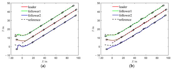
Figure 5.
Trajectories of USVs (Case 1). (a) Method 1; (b) Method 2.
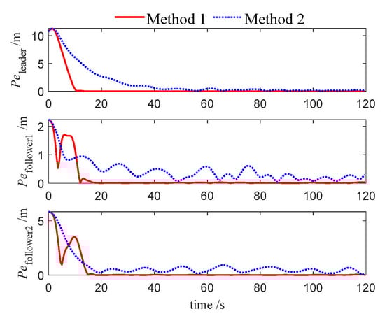
Figure 6.
Tracking errors of USVs (Case 1).
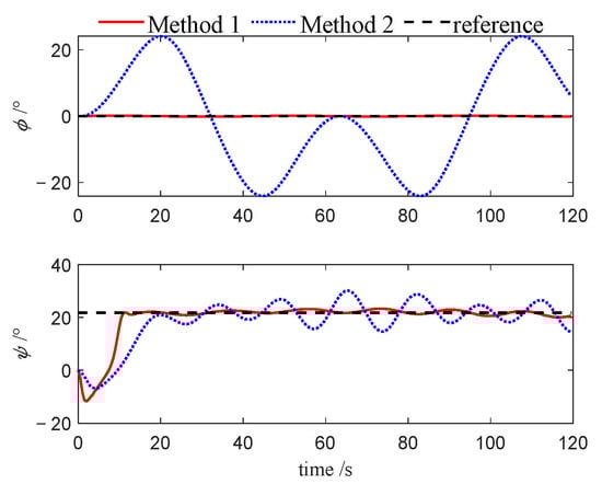
Figure 7.
Attitudes of leader (Case 1).
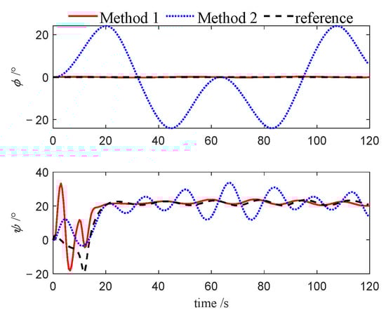
Figure 8.
Attitudes of follower 1 (Case 1).
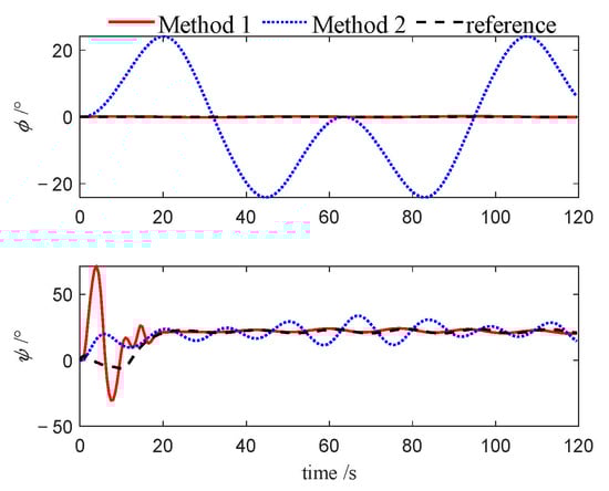
Figure 9.
Attitudes of follower 2 (Case 1).
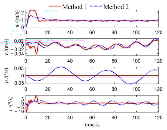
Figure 10.
Velocities of leader (Case 1).
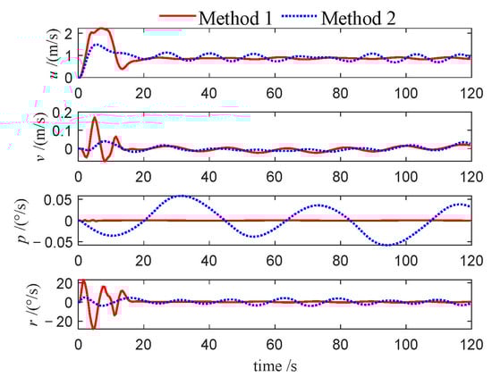
Figure 11.
Velocities of follower 1 (Case 1).
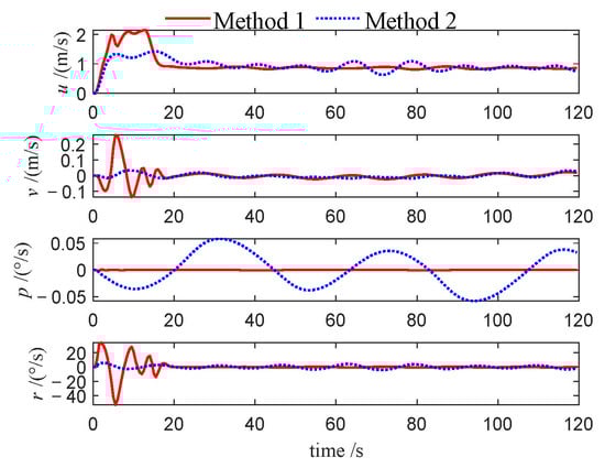
Figure 12.
Velocities of follower 2 (Case 1).
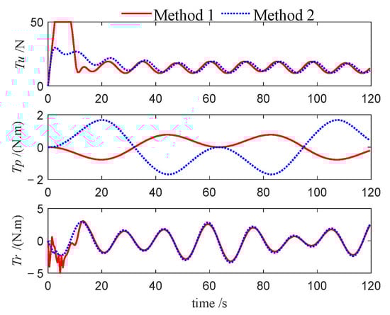
Figure 13.
Control inputs of leader (Case 1).
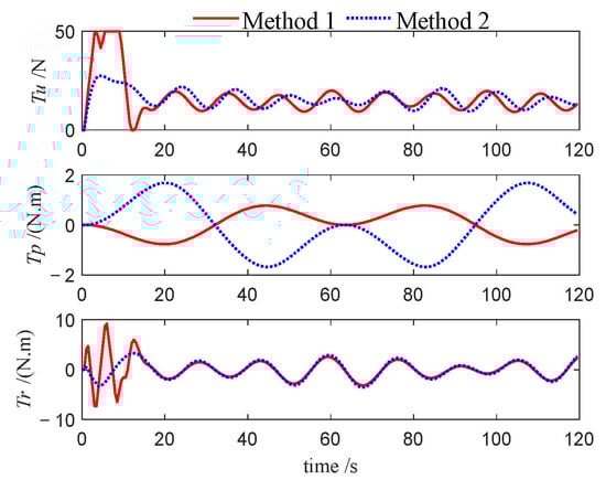
Figure 14.
Control inputs of follower 1 (Case 1).
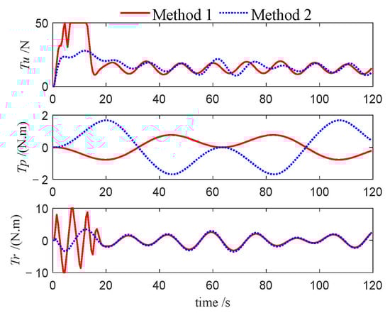
Figure 15.
Control inputs of follower 2 (Case 1).
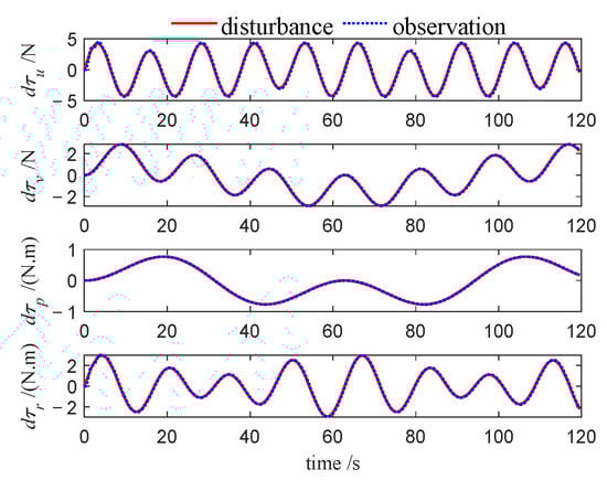
Figure 16.
Disturbances and observations (Case 1).
- Case 2. Circular trajectory
The desired trajectory of the leader USV is described as: . The desired relative positions of the follower USVs with respect to the leader USV are specified as: . The weighting coefficient matrix Q is selected as: , and the initial conditions of USVs are given by:
The simulation results of Case 2 are shown in Figure 17, Figure 18, Figure 19, Figure 20, Figure 21, Figure 22, Figure 23, Figure 24, Figure 25, Figure 26 and Figure 27.
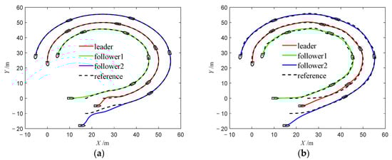
Figure 17.
Trajectories of USVs (Case 2). (a) Method 1; (b) Method 2.
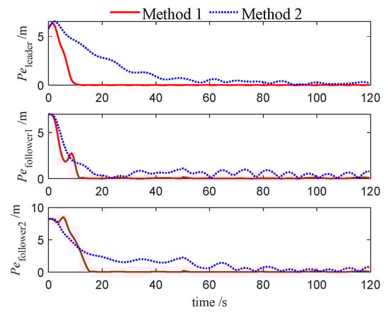
Figure 18.
Tracking errors of USVs (Case 2).
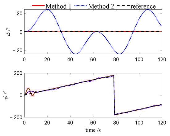
Figure 19.
Attitudes of leader (Case 2).
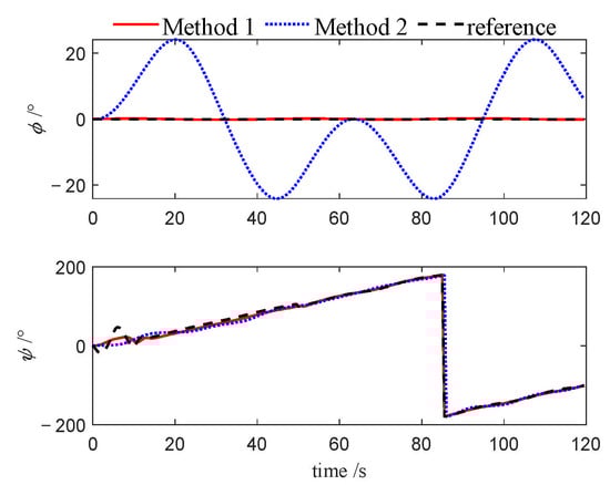
Figure 20.
Attitudes of follower 1 (Case 2).
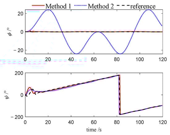
Figure 21.
Attitudes of follower 2 (Case 2).
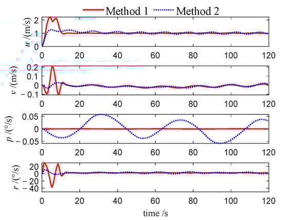
Figure 22.
Velocities of leader (Case 2).
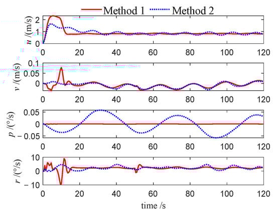
Figure 23.
Velocities of follower 1 (Case 2).
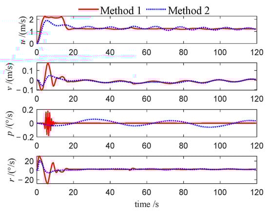
Figure 24.
Velocities of follower 2 (Case 2).
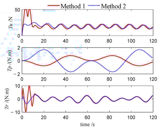
Figure 25.
Control inputs of leader (Case 2).
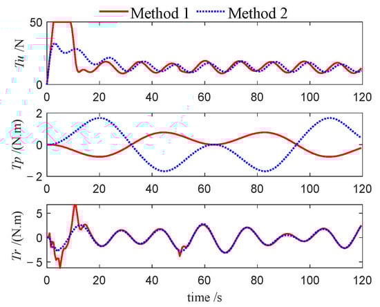
Figure 26.
Control inputs of follower 1 (Case 2).
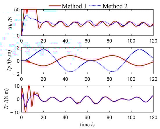
Figure 27.
Control inputs of follower 2 (Case 2).
- Case 3. Sinusoidal trajectory
The desired trajectory of the leader USV is described as: . The desired relative positions of the follower USVs with respect to the leader USV are specified as: . The weighting coefficient matrix Q is selected as: , and the initial conditions of USVs are given by:
The simulation results of Case 3 are shown in Figure 28, Figure 29, Figure 30, Figure 31, Figure 32, Figure 33, Figure 34, Figure 35, Figure 36, Figure 37 and Figure 38.
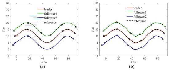
Figure 28.
Trajectories of USVs (Case 3). (a) Method 1; (b) Method 2.
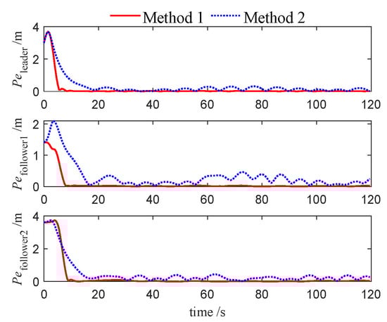
Figure 29.
Tracking errors of USVs (Case 3).
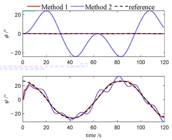
Figure 30.
Attitudes of leader (Case 3).
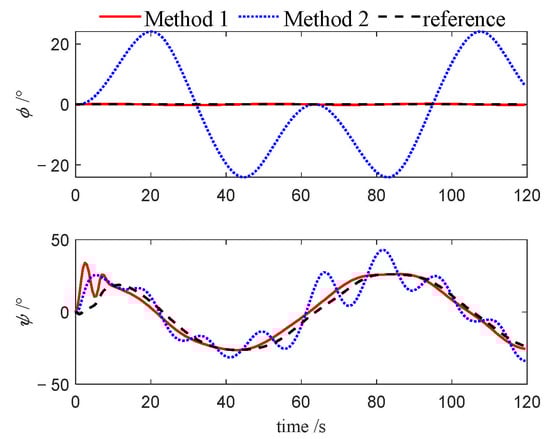
Figure 31.
Attitudes of follower 1 (Case 3).
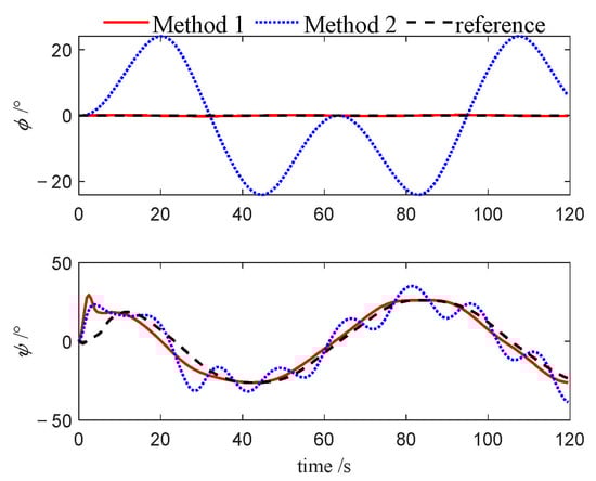
Figure 32.
Attitudes of follower 2 (Case 3).
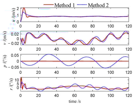
Figure 33.
Velocities of leader (Case 3).
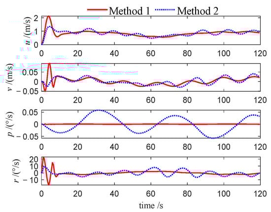
Figure 34.
Velocities of follower 1 (Case 3).
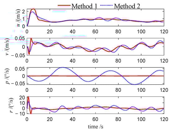
Figure 35.
Velocities of follower 2 (Case 3).
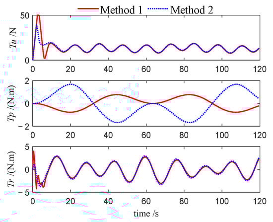
Figure 36.
Control inputs of leader (Case 3).
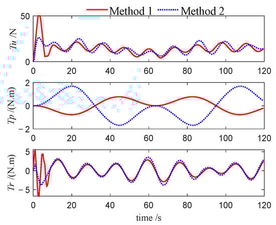
Figure 37.
Control inputs of follower 1 (Case 3).
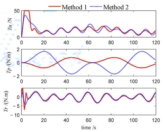
Figure 38.
Control inputs of follower 2 (Case 3).
In the simulation results for the three cases, Figure 5a, Figure 17a and Figure 28a depict the trajectories of the USV formation under Method 1. These results demonstrate that the NMPC algorithm enables the USV formation to accurately track the desired trajectory, thereby verifying the stability and effectiveness of the proposed algorithm. In contrast, Figure 5b, Figure 17b and Figure 28b illustrate the trajectories under Method 2. Compared with Method 1, the USV formation under Method 2 fails to follow the desired trajectory as closely and exhibits more pronounced tracking errors, highlighting the limitations of the PID algorithm in USV tracking control.
Furthermore, Figure 6, Figure 18 and Figure 29 show the evolution of position errors for the USV formation under both control algorithms across the three cases. It is evident that Method 1 consistently yields significantly smaller tracking errors, further confirming the effectiveness and accuracy of the proposed NMPC algorithm for underactuated USV formation tracking control. Additionally, in the aforementioned trajectory Figures, the desired trajectories of the follower USVs remain smooth during the initial tracking phase, reflecting the effectiveness of the tracking differentiator.
Figure 7, Figure 8, Figure 9, Figure 19, Figure 20, Figure 21, Figure 30, Figure 31 and Figure 32 depict the variations in roll and heading angles for the leader USV and two follower USVs across three different cases. It can be observed that, under Method 2, significant periodic errors are present in the roll and heading angles of all three USVs, indicating a lack of convergence in these states when the PID algorithm is applied. In contrast, under Method 1, both the roll and heading angles are accurately tracked to their desired values, further validating that the NMPC algorithm, designed based on the quasi-infinite horizon theory, ensures superior stability and performance compared to the PID algorithm.
This performance gap is further substantiated by the velocity profiles presented in Figure 10, Figure 11, Figure 12, Figure 22, Figure 23, Figure 24, Figure 33, Figure 34 and Figure 35. Compared to Method 1, substantially larger fluctuations in surge, sway, roll, and yaw velocities are observed under Method 2 for all three USVs, which further highlights the limitations of the PID algorithm in maintaining velocity stability. The variations in control inputs for the three USVs are presented in Figure 13, Figure 14, Figure 15, Figure 25, Figure 26, Figure 27, Figure 36, Figure 37 and Figure 38. It can be observed that, under the NMPC-based control, larger control inputs are applied during the initial tracking phase, allowing the USV formation to be driven to the desired trajectory with a faster response speed.
To facilitate a quantitative evaluation of the controller’s performance, four metrics were adopted in this study: the mean steady-state error (MSSE), the root mean square error (RMSE) of tracking error, the convergence time, and the overshoot. The comparative results, summarized in Table 3, Table 4 and Table 5, provide clear and compelling evidence of the superiority of the proposed NMPC-based method (Method 1) over the PID-based approach (Method 2).
Table 3.
Performance metrics comparison in Case 1.
Table 4.
Performance metrics comparison in Case 2.
Table 5.
Performance metrics comparison in Case 3.
In terms of tracking accuracy, Method 1 consistently achieves significantly lower MSSE and RMSE across all three test cases. For instance, in the Case 3, the leader USV’s MSSE was reduced by over 80% (from 0.142 m to 0.023 m), a trend that holds for the follower USVs and for the Case 1 and Case 2. This demonstrates a marked improvement in the formation’s ability to precisely maintain its desired position. Furthermore, the proposed method exhibits a faster and more stable dynamic response. Convergence times under Method 1 are drastically shorter, with reductions of up to 75% (e.g., from 41 s to 10 s for the leader in Case 1). This faster convergence indicates a more stable and efficient control action.
The observed quantitative improvements can be directly linked to the theory of the proposed control architecture. The exceptional robustness and significantly lower mean steady-state errors (MSSE) are a direct consequence of the finite-time disturbance observer. As shown in Figure 16, the observer accurately estimates and compensates for the unknown marine disturbances in real-time, fulfilling its theoretical purpose of enhancing disturbance rejection. This active compensation allows the USVs to maintain their desired trajectories with high precision, even in the presence of external forces.
Furthermore, the superior dynamic response is attributable to the predictive nature of the quasi-infinite horizon NMPC. Unlike a reactive controller, the NMPC optimizes the control inputs over a future horizon, anticipating the desired trajectory. This proactive approach allows for aggressive yet smooth control actions that guide the USVs to the reference trajectory quickly without the significant overshoot. The stability guarantees from the quasi-infinite horizon design ensure this aggressive response does not lead to instability. Finally, the effectiveness of the tracking differentiator is evident in the smooth initial trajectories of the follower USVs, which helps prevent large initial tracking errors and contributes to the overall stability and reduced overshoot of the formation. Collectively, the simulation results provide concrete validation of the expected theoretical benefits of each component of our integrated control strategy.
6. Conclusions
This paper successfully developed and validated a robust cooperative formation control strategy for underactuated USVs by explicitly addressing the critical effects of roll motion. The main contribution lies in the design and rigorous stability analysis of a quasi-infinite horizon Nonlinear Model Predictive Control (NMPC) framework for a four-degree-of-freedom (4-DOF) USV model. The mathematical core of this contribution is the construction of a terminal penalty function and terminal inequality constraints based on quasi-infinite horizon theory, which, combined with a Lyapunov-based analysis, formally guarantees the stability of the closed-loop system within a finite prediction horizon. The integration of a finite-time disturbance observer further enhances the system’s robustness against unknown marine disturbances. To further enhance the tracking performance of the followers, a tracking differentiator is designed to smooth the heading angle of the leader USV when generating the desired trajectories for the followers.
The superiority of the proposed method was demonstrated through comparative simulations against a conventional PID controller. The quantitative results were compelling: our approach reduced the mean steady-state error (MSSE) by over 80% in some cases (e.g., from 0.142 m to 0.023 m for the leader USV in the Case 3) and shortened convergence times by as much as 75% (e.g., from 41 s to 10 s). Quantitative analysis of performance metrics, including tracking error, convergence time, and overshoot, confirms that the proposed algorithm offers substantial improvements over traditional control methods, ensuring more precise and stable formation control.
Building upon the theoretical framework and simulation results presented in this paper, several promising avenues for future research emerge. A critical next step involves conducting comprehensive experimental validation of the proposed control algorithms on a physical multi-USV testbed. Such experiments will be crucial for verifying the real-world robustness and practical applicability of our method. Furthermore, we intend to extend our investigation to address the challenges of formation control in low-communication environments, considering aspects such as limited bandwidth, intermittent connectivity, and communication delays. Finally, exploring the complexities of heterogeneous formation control, where the USV team comprises vessels with diverse dynamic characteristics, sizes, and operational capabilities, represents another significant direction to broaden the applicability and impact of this research.
Author Contributions
Conceptualization, M.Y. and R.L.; methodology, M.Y. and R.L.; software, R.L.; validation, M.Y., R.L. and H.W.; formal analysis, M.Y.; investigation, R.L.; resources, M.Y.; data curation, H.W. and R.L.; writing—original draft preparation, M.Y. and R.L.; writing—review and editing, M.Y., H.W. and Z.D.; visualization, W.L. and Z.D.; supervision, H.W.; project administration, H.W.; funding acquisition, H.W. All authors have read and agreed to the published version of the manuscript.
Funding
This research was funded by the Hubei Provincial Natural Science Foundation Youth Category A under Grant No. 2025AFA117, the Key Support Project of Hanjiang National Laboratory (No. ZC2024011), and the China State Shipbuilding Corporation (CSSC) Special Support Project for Hanjiang Laboratory (No. JZ2024009).
Data Availability Statement
The original contributions presented in this study are included in the article. Further inquiries can be directed to the corresponding author.
Acknowledgments
The authors gratefully acknowledge the support provided by the Hubei Provincial Natural Science Foundation, the Key Support Project of Hanjiang National Laboratory and the CSSC Special Support Project for Hanjiang Laboratory.
Conflicts of Interest
The authors declare no conflicts of interest.
References
- Peng, Z.; Wang, J.; Wang, D.; Han, Q.L. An overview of recent advances in coordinated control of multiple autonomous surface vehicles. IEEE Trans. Ind. Inform. 2020, 17, 732–745. [Google Scholar] [CrossRef]
- Gao, S.; Peng, Z.; Liu, L.; Wang, D.; Han, Q.L. Fixed-time resilient edge-triggered estimation and control of surface vehicles for cooperative target tracking under attacks. IEEE Trans. Intell. Veh. 2023, 8, 547–556. [Google Scholar] [CrossRef]
- Ghommam, J.; Saad, M.; Mnif, F.; Zhu, Q.M. Guaranteed performance design for formation tracking and collision avoidance of multiple USVs with disturbances and unmodeled dynamics. IEEE Syst. J. 2020, 15, 4346–4357. [Google Scholar] [CrossRef]
- Jiang, Y.; Liu, Z.; Chen, F. Adaptive output-constrained finite-time formation control for multiple unmanned surface vessels with directed communication topology. Ocean Eng. 2024, 292, 116552. [Google Scholar] [CrossRef]
- Batkovic, I.; Ali, M.; Falcone, P.; Zanon, M. Safe trajectory tracking in uncertain environments. IEEE Trans. Autom. Control 2022, 68, 4204–4217. [Google Scholar] [CrossRef]
- Jiang, X.; Xia, G.; Feng, Z.; Wu, Z.G. Nonfragile formation seeking of unmanned surface vehicles: A sliding mode control approach. IEEE Trans. Netw. Sci. Eng. 2021, 9, 431–444. [Google Scholar] [CrossRef]
- Shen, H.; Yin, Y.; Qian, X. Fixed-time formation control for unmanned surface vehicles with parametric uncertainties and complex disturbance. J. Mar. Sci. Eng. 2022, 10, 1246. [Google Scholar] [CrossRef]
- Sui, B.; Zhang, J.; Liu, Z.; Wei, J. Distributed prescribed-time cooperative formation tracking control of networked unmanned surface vessels under directed graph. Ocean Eng. 2024, 305, 117993. [Google Scholar] [CrossRef]
- Duan, H.; Yuan, Y.; Zeng, Z. Distributed robust learning control for multiple unmanned surface vessels with fixed-time prescribed performance. IEEE Trans. Syst. Man Cybern. Syst. 2023, 54, 787–799. [Google Scholar] [CrossRef]
- Dong, Z.P.; Qi, S.J.; Yu, M.; Zhang, Z.Q.; Zhang, H.S.; Li, J.K.; Liu, Y. An improved dynamic surface sliding mode method for autonomous cooperative formation control of underactuated USVs with complex marine environment disturbances. Pol. Marit. Res. 2022, 29, 47–60. [Google Scholar] [CrossRef]
- Xia, G.; Zhang, Y.; Zhang, W.; Chen, X.; Yang, H. Dual closed-loop robust adaptive fast integral terminal sliding mode formation finite-time control for multi-underactuated AUV system in three dimensional space. Ocean Eng. 2021, 233, 108903. [Google Scholar] [CrossRef]
- Dong, Z.; Zhou, W.; Tan, F.; Wang, B.; Wen, Z.; Liu, Y. Simultaneous modeling and adaptive fuzzy sliding mode control scheme for underactuated USV formation based on real-time sailing state data. Ocean Eng. 2024, 314, 119743. [Google Scholar] [CrossRef]
- Huang, X.; Liu, H.; Tian, X.; Yuan, J. Guiding vector field and self-structuring learning network-based formation control of underactuated surface vessels in static obstacle environments with flexible performances. ISA Trans. 2024, 153, 96–116. [Google Scholar] [CrossRef] [PubMed]
- Dong, Z.; Tan, F.; Zhou, W.; Wang, B.; Liu, Y. Distributed formation control of underactuated UMVs based on nonlinear model prediction algorithm with obstacle avoidance strategy incorporating relative velocity constraints. Ocean Eng. 2024, 312, 119272. [Google Scholar] [CrossRef]
- Yuan, S.; Liu, Z.; Sun, Y.; Song, S.; Wang, Z.; Zheng, L. EMPMR berthing scheme: A novel event-triggered motion planning and motion replanning scheme for unmanned surface vessels. Ocean Eng. 2023, 286, 115666. [Google Scholar] [CrossRef]
- Wang, L.; Xu, X.; Han, B.; Zhang, H. Multiple autonomous underwater vehicle formation obstacle avoidance control using event-triggered model predictive control. J. Mar. Sci. Eng. 2023, 11, 2016. [Google Scholar] [CrossRef]
- Zhang, M.; Yan, Z.; Zhou, J.; Yue, L. Distributed dual closed-loop model predictive formation control for collision-free multi-AUV system subject to compound disturbances. J. Mar. Sci. Eng. 2023, 11, 1897. [Google Scholar] [CrossRef]
- Yan, Z.; Yan, J.; Nan, F.; Cai, S.; Hou, S. Distributed TMPC formation trajectory tracking of multi-UUV with time-varying communication delay. Ocean Eng. 2024, 297, 117091. [Google Scholar] [CrossRef]
- Li, S.; Zhu, Y.; Bai, J.; Guo, G. Dynamic obstacle avoidance of unmanned ship based on event-triggered adaptive nonlinear model predictive control. Ocean Eng. 2023, 286, 115626. [Google Scholar] [CrossRef]
- Zhu, Y.; Li, S.; Guo, G.; Yuan, P.; Bai, J. Formation control of UAV–USV based on distributed event-triggered adaptive MPC with virtual trajectory restriction. Ocean Eng. 2024, 294, 116850. [Google Scholar] [CrossRef]
- Liu, C.; Hu, Q.; Sun, T. Distributed formation control of underactuated ships with connectivity preservation and collision avoidance. Ocean Eng. 2022, 263, 112350. [Google Scholar] [CrossRef]
- Gonzalez-Garcia, A.; Collado-Gonzalez, I.; Cuan-Urquizo, R.; Sotelo, C.; Sotelo, D.; Castaneda, H. Path-following and LiDAR-based obstacle avoidance via NMPC for an autonomous surface vehicle. Ocean Eng. 2022, 266, 112900. [Google Scholar] [CrossRef]
- Perez, T.; Fossen, T. Kinematic models for maneuvering and sea keeping of marine vessels. Model. Identif. Control 2007, 28, 19–30. [Google Scholar] [CrossRef]
- Consolini, L.; Morbidi, F.; Prattichizzo, D.; Tosques, M. Leader-follower formation control of nonholonomic mobile robots with input constraints. Automatica 2008, 44, 1343–1349. [Google Scholar] [CrossRef]
- Xia, G.; Sun, C.; Zhao, B.; Xue, J. Cooperative control of multiple dynamic positioning vessels with input saturation based on finite-time disturbance observer. Int. J. Control Autom. Syst. 2019, 17, 370–379. [Google Scholar] [CrossRef]
- Wei, H.; Shen, C.; Shi, Y. Distributed Lyapunov-based model predictive formation tracking control for autonomous underwater vehicles subject to disturbances. IEEE Trans. Syst. Man Cybern. Syst. 2021, 51, 5198–5208. [Google Scholar] [CrossRef]
Disclaimer/Publisher’s Note: The statements, opinions and data contained in all publications are solely those of the individual author(s) and contributor(s) and not of MDPI and/or the editor(s). MDPI and/or the editor(s) disclaim responsibility for any injury to people or property resulting from any ideas, methods, instructions or products referred to in the content. |
© 2025 by the authors. Licensee MDPI, Basel, Switzerland. This article is an open access article distributed under the terms and conditions of the Creative Commons Attribution (CC BY) license (https://creativecommons.org/licenses/by/4.0/).