Design of a Sliding Mode Controller for Lateral Motion Control of a Supercavitating Vehicle Based on a Radial Basis Function Neural Network Observer

Abstract

Newton’s second law has been applied to create a dynamic model of the lateral motion of a supercavitating vehicle, assuming a stable cavity. However, some states cannot be measured, and there is uncertainty in the lateral model. Aiming to resolve these issues, this work describes the design of a sliding-mode controller based on a state observer and a radial basis function neural network observer to realize lateral attitude control of supercavitating vehicle. Because there is a variable signal that cannot always be obtained in the established lateral model, the state observer is designed to estimate the unknown state; when there are unknown variables and model uncertainty and the state is unknown, the radial basis function neural network observer estimates model uncertainty. Finally, based on these results, a robust sliding mode controller is designed and system stability is proved by the Lyapunov theorem.

1. Introduction

Compared with traditional underwater vehicles, supercavitating vehicles have dramatically reduced drag and significantly enhanced range and velocity. Recent research mainly focuses on control of longitudinal motion, and work on the control of lateral motion of supercavitating vehicles is rare.

To realize stable control of lateral motion for a supercavitating vehicle, cavity shape and force acting on the vehicle are analyzed and a mathematical model is established. In the cruise stage, the main forces acting on the cavitator and fins are gravity and the planing force induced by the interaction between the aft body and the cavity wall. By contrast, in the lateral plane, there is no gravity factor in the force equation. Therefore, the analysis of lateral dynamics is also based on cavitation theory.

Logvinovich [1] first researched the cavitation phenomenon of supercavitating vehicles, and a large number of experiments and analytical works have since been carried out. A dynamic model of the vehicle based on the states of the force actings was established; simultaneously, a cavity-dependent expression principle based on potential flow theory was presented, and this expression was used to create a calculation model for each cavity section.

Kirschner et al. [2] analyzed the hydrodynamic forces acting on the cavitator, fins and wet area of the aft body; combining these hydrodynamic models, a 6DOF model was established and travel states were predicted by simulation. Vasin et al. [3] focused on the aft part of the immersed surface of the vehicle., established the planing force model, specified the planing force related to immersion depth and immersion angle, and provided the formula to calculate planing force.

Goel [4] assumed that the cavity’s center axis would correspond with the vehicle’s longitudinal axis and established a 6DOF mathematical model, then specified that the supercavitating vehicle was unstable without control.

Savchenko et al. [5] analyzed the different ways to generate transverse control force on a supercavitating vehicle, investigated maneuverability with the minimum turning radius, and studied the cavity-deforming characteristic in the lateral and longitudinal directions under rotary motion. Another study [6] further examined the stability of lateral motion and longitudinal motion under the cavity-deforming condition. A vector-thrust method was adopted to control the stable motion of supercavitating vehicles.

Li et al. [7] focused on the longitudinal motion and lateral motion of supercavitating vehicles, presented a 3D cavity-topology model to predict cavity shape, improved the planing-force model, and simulated the maneuver state by numerical simulation.

Mirzaei [8], aiming to address the low efficiency of fin control, presented a turning-control strategy for supercavitating vehicle without fins, where the fin control surface was substituted by a swing inside the vehicle. These authors also designed a sliding mode controller to track the desired yaw angle.

Song et al. [9] proposed a control strategy with active banking in turns for the 6DOF model of supercavitating vehicle, adopted a three-channel PID controller for maneuver control, and limited the amplitude of the actuator to avoid surpassing the physical bounds.

Luo et al. [10] and Gao et al. [11] established a lateral plane model for the cruise stage of supercavitating vehicle, used the limit rudder method, and designed a PI controller to control the yaw angle. The control method is simple; however, if the deflection angle of the rudder became too large, the system would lose stability. Chen et al. [12], to suppress roll movement, established a roll-movement model for supercavitating vehicles and designed a PD controller to control the cavitator surface to eliminate roll movement induced by gravity-center offset.

Bai et al. [13] analyzed the dynamic characteristics of the horizonal plane and established a dynamic model. Exact feedback linearization was used for the nonlinear part of the model, and the pole-placement method was utilized for yaw control.

To sum up, at present, research on lateral motion control for supercavitating vehicles is rare; moreover, there is no common model for lateral motion to parallel the longitudinal motion control model proposed by Dzielski [14] for controller design. Therefore, more attention should be paid to lateral motion control in supercavitating vehicles.

In this paper, modeling and control of the lateral motion of supercavitating vehicles were studied. In order to investigate the dynamic model of lateral movement, a general model incorporating movement in space, the cavity stream, and the shape of the cavity was adapted to determine the equations defining the cavity’s symmetric axis, radius, maximum radius (plate cavitator), and length. A coordinate system is presented; the hydrodynamic force of a supercavitating vehicle in the lateral plane was analyzed in a system including the lateral component of cavitator force, fin force, and planing force. Then, a lateral dynamic model was established; in lateral movement, the stern rudder was used as an actuator of attitude control and a sliding mode variable structure as adopted as the controller. As measurements of slide side angle and yaw rate are inaccurate or even non-acquirable, a state observer was designed to estimate slide side angle and yaw rate. As there is still uncertainty and unmeasurable signal in the model, a radial basis function neural network observer was designed, with the observer used to observe the unknown variant and the radial basis function neural network used to estimate the uncertain variables. Then, based on the estimated value, a sliding mode variable structure controller was designed to realize control of lateral trajectory tracking. The stability of the control system was proven by the Lyapunov theorem, and the robustness and tracking performance of the control system were verified by simulation.

2. Lateral Dynamic Model of a Supercavitating Vehicle

2.1. General Cavity Form in Motion in Space

In motion in 3D space, the state of a supercavitating vehicle varies with time; therefore, there is a center offset between each cavity section and the body section that affects cavity shape. For cavity shape to be studied, the cavity-section center must be determined, as must the cavity axis, cavity radius, cavity length, and maximum radius.

(1)

Cavity axis equation

$$\begin{array}{c}\begin{array}{c}{R}_{1y}\left(t\right)={\displaystyle \frac{v}{{\omega }_z}}\left(\sqrt{1-{\left({\displaystyle \frac{{\omega }_z{x}_1}{v}}\right)}^2}-1\right)+{\displaystyle \frac{1}{3}}\left(1+\sigma \right){\displaystyle \frac{{\omega }_z{x}_1^2}{v}}+{\displaystyle \frac{\left(1+\sigma \right)x_1^2}{3F{r}_L^2{L}_c}}-\\ R_n{C}_{x0}\left(1+\sigma \right)\left(0.23-0.5\sigma +{\displaystyle \frac{x_1}{L_c}}\right)\mathit{sin}2{\alpha }_n\end{array}\\ \begin{array}{ll}{R}_{1z}\left(t\right)=& {\displaystyle \frac{v}{{\omega }_y}}\left(\sqrt{1-{\left({\displaystyle \frac{{\omega }_y{x}_1}{v}}\right)}^2}-1\right)+{\displaystyle \frac{1}{3}}\left(1+\sigma \right){\displaystyle \frac{{\omega }_y{x}_1^2}{v}}+\\ & R_n{C}_{x0}\left(1+\sigma \right)\left(0.23-0.5\sigma +{\displaystyle \frac{x_1}{L_c}}\right)\mathit{sin}2{\beta }_n\\ & 0\le x_1\le L_c\end{array}\end{array}$$

(1)

where $R_{1y}\left(t\right)$ and $R_{1z}\left(t\right)$ are the center coordinates of the cavity section $v$ is the travel speed of the vehicle; ${\omega }_z$ is the pitch rate; $\sigma$ is the cavitation number; $L_c$ is the cavity length; $C_{x0}$ is the drag coefficient at cavitation zero; $R_n$ is the cavitator radius; ${\omega }_y$ is the yaw rate; $F{r}_L$ is the Froude number; ${\alpha }_n$ is the attack angle of the cavitator; and ${\beta }_n$ is the slide side angle of the cavitator, which can be calculated by ${\beta }_n={\delta }_c+\beta$.

(2)

Cavity radius equation along the cavity axis

$$R\left(x_1\right)=R_c\sqrt{1-\left(1-\left({\displaystyle \frac{R_n^2}{R_c^2}}\right){\left(1-{\displaystyle \frac{2x_1}{L_c}}\right)}^{{\displaystyle \frac{2}{\eta }}}\right)}, 0\le x_1\le L_c$$

(2)

(3)

Maximum radius equation of the cavity for the plate cavitator

$$R_c=R_n\sqrt{{\displaystyle \frac{C_x}{k\sigma }}},k={\displaystyle \frac{1+50\sigma }{1+56.2\sigma }}$$

(3)

(4)

Cavity length

$$L_c={\displaystyle \frac{2R_n}{\sigma }}\sqrt{C_x\mathit{ln}{\displaystyle \frac{1}{\sigma }}}$$

(4)

$\eta$ is the correlation coefficient, ${\delta }_c$ is the deflection angle of the cavitator, and $C_x$ is the drag coefficient.

2.2. Analyses of Acting Forces in Lateral Motion

With the object of elucidating the lateral 2 DOF mathematical model of supercavitation, the actual vehicle is simplified into parts, as follows: the cavitator (mounted on the head of the body); the body of the vehicle, which is further subdivided into the conical section and the cylindrical section; and the aft part, which contains the rudder. The cavitator and rudder act as actuators to stabilize the motion of the vehicle. The force diagram of the vehicle is shown in Figure 1.

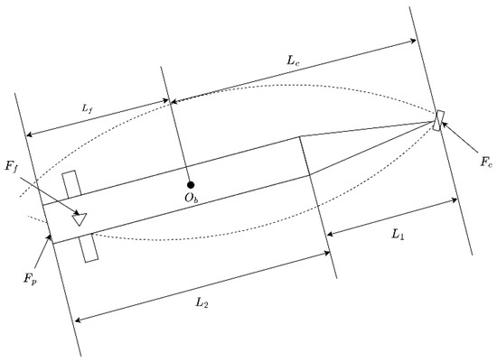
Figure 1. Force diagram of the vehicle.

In this diagram, $L_1$ is the length of the conical section, $L_1=L/3$, and $L_2$ is the length of the cylindrical section, $L_2=2L/3$,$L=L_1+L_2$. The distance between the mass center of the vehicle and the center of the cavitator is $L_c=17L/28$, and the distance between the mass center of the vehicle and the tail part is $L_f=11L/28$. The mass center of the vehicle is the origin of the body coordinate; therefore, the lateral forces of the supercavitating vehicle are the hydrodynamic force of the cavitator, the hydrodynamic force of the fins, and the planing force induced by interactions between the tail part and the cavity wall, along with the corresponding moment of the above three kinds of force.

(1)

Cavitator force

The cavitator is an important component of a supercavitating vehicle. In this paper, the cavitator is a plate cavitator, the lateral hydrodynamic force of which is shown in Figure 2.

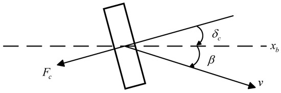
Figure 2. Diagram of the hydrodynamic force of the cavitator.

The hydrodynamic force of the cavitator is found as follows [15]:

$$F_c=0.5\rho v^2{S}_c{c}_y^n\left({\delta }_c+\beta \right)$$

(5)

The moment of the cavitator hydrodynamic force is found as follows:

$$M_y^n=-0.5\rho v^2{S}_c{c}_y^n{\delta }_c{L}_c$$

(6)

where $\rho$ is the fluid density, $S_c$ is the transection of the cavitator, $c_y^n$ is the lift coefficient of the cavitator, let $c_y^n=C_x$, ${\delta }_c$ is the deflection angle of the cavitator, $\beta$ is the slide side angle of the vehicle, and ${\beta }_n={\delta }_c+\beta$ is the slide side of the cavitator.

(2)

Hydrodynamic of the fins

The fins of the vehicle form a cross rudder consisting of a pair of vertical rudders and a pair of horizonal rudders. Horizonal rudders mainly control the motion of the vehicle in the longitudinal plane; for this paper, which focuses on lateral motion, vertical rudders were adopted to control the vehicle. Vertical rudders also control the roll movement of the vehicle. Roll movement was neglected, and only placement and yaw rotation of lateral movement were considered. The research work is divided into two parts. In part one, the fins are divided into an upper rudder and a lower rudder, which are considered as differential rudders, and force analysis is carried out for them. In part two, the fins are considered as a whole unit—a stern rudder—in the analysis of the force conditions.

Forces acting on the fins are divided into lateral forces on the upper rudder and the lower rudder. The hydrodynamic forces induced by deflection of the upper rudder are shown in Figure 3.

Figure 3. Diagram of hydrodynamic forces acting on the upper rudder.

When we analyze the hydrodynamic force acting on the fins, fins can be considered as a special cavitator, so the same method was adopted to analyze the force on the fins. The force acting of the upper rudder is calculated as follows:

$$F_{sd}=0.5\rho v^2{S}_c{c}_z^{sd}({\delta }_{fs}-\beta -{\displaystyle \frac{{\omega }_y{L}_f}{v}})$$

(7)

The moment produced by the upper rudder is calculated as follows:

$$M_y^{sd}=F_{sd}{L}_f$$

(8)

In the same way, the lateral force and moment produced by lower rudder are calculated as follows:

$$F_{xd}=0.5\rho v^2{S}_c{c}_z^{xd}({\delta }_{fx}-\beta -{\displaystyle \frac{{\omega }_y{L}_f}{v}})$$

(9)

$$M_y^{xd}=F_{xd}{L}_f$$

(10)

where $c_z^{sd}$ is the lateral force coefficient of the upper rudder, ${\delta }_{fs}$ is the deflection angle of the upper rudder, $c_z^{xd}$ is the lateral force coefficient of the lower rudder, ${\delta }_{fx}$ is the deflection angle of the lower rudder, $c_z^{sd}=n_1{C}_x,c_z^{xd}=n_2{C}_x, \mathrm{a}\mathrm{n}\mathrm{d} n_1$ and $n_2$ are the coefficients of effectiveness relative to the cavitator of the upper rudder and lower rudder, respectively. The coefficient is a value obtained from the experimental literature [14]. In practice, the actual upper rudder and lower rudder are not exactly same; therefore, $n_1$ and $n_2$ are set to 0.4 and 0.6.

Considering the fins as stern rudders, in this way, the direction and value of deflection angle of the upper and lower rudder are same as those of the stern rudder, that is, the stern rudder acts as an actuator. The stern rudder is considered as a special cavitator too; therefore, the lateral force acting on stern rudder is as follows:

$$F_f=0.5\rho v^2{S}_c{c}_z^d({\delta }_f-\beta -{\displaystyle \frac{{\omega }_y{L}_f}{v}})$$

(11)

The moment produced by the stern rudder is as follows:

$$M_y^d=F_f{L}_f$$

(12)

where $c_z^d$ is the lateral force coefficient, $c_z^d=n_3{C}_x$, $n_3$ is coefficient of effectiveness of the stern rudder relative to the cavitator, $n_3=0.5$, and ${\delta }_f$ is the deflection angle of the stern rudder. The deflection angles of the upper and lower rudder are equivalent to the deflection angle of the stern rudder, and the formula is as follows:

$${\delta }_f={\displaystyle \frac{{\delta }_{fs}+{\delta }_{fx}}{2}}$$

(13)

Later, the control effects of the differential rudder as the actuator and the stern rudder as the actuator of the system are analyzed.

(3)

Planing force

When a supercavitating vehicle conducts yaw movement, the tail part and cavity wall interact with each other to generate planing force. Planing force differs from cavitator force and fin force, and it depends on the impact on the tail part and cavity wall, that is, it is related to cavity state and vehicle attitude. The magnitude of the planing force is determined by the length of the tail body through the cavity wall, the immersion angle between the vehicle and cavity wall, and the attitude of the vehicle, and the planing force is a nonlinear force. In this paper, the modeling of planing force is derived from the 3DOF planing force and then divided into a lateral planing force. The diagram of planing force is shown in Figure 4.

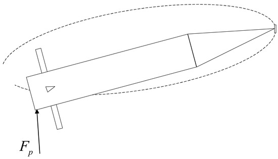
Figure 4. Diagram of planing force.

The planing force generated by the interaction between the tail part and the cavity wall is as follows [15]

$$F_p=-\pi \rho v^2{r}_{ke}^2\mathit{sin}{\alpha }_w\mathit{cos}{\alpha }_w({\displaystyle \frac{R_b+h_e}{R_b+2h_e}})(1-({\displaystyle \frac{\xi }{\xi +h_e}}{)}^2)$$

(14)

$F_p$ is the total planing force; the lateral planing force $F_{pz}$ is the substance of the total planing force along $O_b{z}_b$ in the body coordinate, as follows:

$$F_{pz}=-\pi \rho V^2{r}_{ke}^2\mathit{sin}{\alpha }_w\mathit{cos}{\alpha }_w({\displaystyle \frac{R_b+h_e}{R_b+2h_e}})(1-({\displaystyle \frac{\xi }{\xi +h_e}}{)}^2)\mathit{sin}{\theta }_{sp}$$

(15)

where $\xi$ is the difference between the cavity radius and the shell radius of the tail parts of the vehicle.

$$\xi =r_{ke}-R_b$$

(16)

$r_{ke}$ and $R_b$ are the cavity radius and shell radius of the tail parts, respectively. $h_e$ is the immersion depth, calculated as follows:

$$h_e=R_b+\sqrt{R_{1y}^2+R_{1z}^2}-r_{ke}$$

(17)

$R_{1y}$ and $R_{1z}$ are the horizontal and vertical coordinates of the cavity section center at the tail part.

In (15), ${\theta }_{sp}$ is the contacting angle between the cavity and the transection shell where the planing force acts; it is defined as an angle between the line jointed vehicle center and the cavity center in cross section, with an axis of $O_b{y}_b$ in the body coordinate, as shown in Figure 5.

$${\theta }_{sp}=\mathit{arctan}\left|{\displaystyle \frac{R_{1z}}{R_{1y}}}\right|$$

(18)

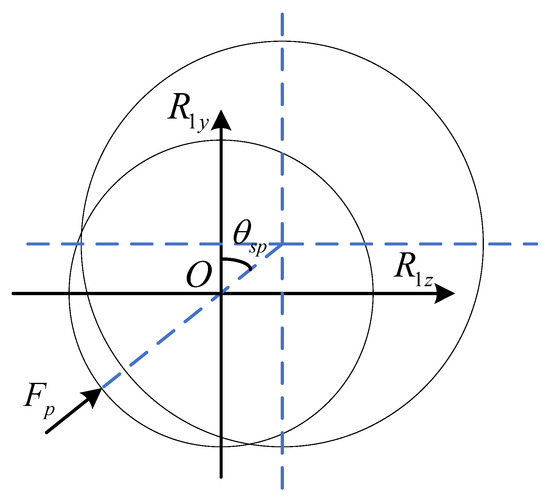
Figure 5. Relative location between vehicle tail and cavity.

Because this paper mainly investigates lateral movement, pitch rate and attack angle of the cavitator in longitudinal movement are not described. Therefore, $R_{1y}$ is unknown and assumed to be stable in longitudinal movement, and the center coordinate of the cavity section is $R_{1ym}=0.02$ when the vehicle is still inside the cavity. Because $R_{1ym}$ is a small variable relative to the length of the vehicle, it is assumed to increase linearly from the cavitator center to the center coordinate of the cavity section of the tail part. The relationship between the longitudinal coordinate of the cavity section center and the vehicle axis is shown in Figure 6.

Figure 6. Longitudinal coordinate of the cavity section.

The center longitudinal coordinate of the cavity section at $x_1$ of the transection of the vehicle is as follows:

$$R_{1y}\left(x_1\right)={\displaystyle \frac{R_{1ym}}{L_1}}$$

(19)

In (15), ${\alpha }_w$ is the immersion angle, expressed as follows:

$${\alpha }_w=\mathit{arctan}{\displaystyle \frac{h_e}{l_w}}$$

(20)

where $l_w$ is the immersion length. In order to obtain the immersion length of the tail shell, the distance $x_{10}$ between the cavitator center and the location of the section when immersion length is equal to zero should be determined. $x_{10}$ is calculated as follows:

$$R_b+\sqrt{{\left(R_{1y}\left(x_{10}\right)\right)}^2+{\left(R_{1z}\left(x_{10}\right)\right)}^2}-r_k\left(x_{10}\right)=0$$

(21)

Therefore, immersion length is calculated as follows:

$$l_w=L-x_{10}$$

(22)

The moment generated by the planing force is as follows:

$$M_{pz}=F_{pz}{L}_w$$

(23)

2.3. Generation of Dynamic Model

According to Newton’s second law and the definition of momentum, the dynamic equation for a supercavitating vehicle is obtained as follows:

$$\begin{array}{c}mv\left({\omega }_y-\dot{\beta }\right)=-F_z\\ J{\dot{\omega }}_y=M_y\end{array}$$

(24)

where $m$ is vehicle mass and $J$ is rotation inertia about $O_b{y}_b$. $m$ and $J$ are expressed as follows:

$$m={\displaystyle \frac{7}{9}}{\rho }_{b}v\pi R_b^{2}L$$

(25)

$$J={\displaystyle \frac{11}{60}}{\rho }_b\pi R_b^{4}L+{\displaystyle \frac{133}{405}}{\rho }_b\pi R_b^2{L}^3$$

(26)

where ${\rho }_b$ is the density of the vehicle and $R_b$ is the radius of the cylinder section.

In Equation (24), $F_z$ and $M_y$ are total force and total moment. They are as follows:

$$F_z=F_c+F_{sd}+F_{xd}+F_{pz}$$

(27)

$$M_y=M_y^n+M_y^{sd}+M_y^{xd}+M_{pz}$$

(28)

where force $F_c,F_{sd},F_{xd},F_{pz}$ are cavitator force, fin force and planing force, and $M_y^n,M_y^{sd},M_y^{xd},M_{pz}$ are the corresponding moments.

A mathematical model is obtained by combining the dynamic model and the kinematics model of a supercavitating vehicle in the horizontal plane. Transforming the mathematical model into matrix form yields the following:

$$\left[\begin{array}{c}\dot{\beta }\\ {\dot{\omega }}_y\\ \dot{\psi }\end{array}\right]=\left[\begin{array}{ccc}{a}_{11}& a_{12}& 0\\ a_{21}& a_{22}& 0\\ 0& 1& 0\end{array}\right]\left[\begin{array}{c}\beta \\ {\omega }_y\\ \psi \end{array}\right]+\left[\begin{array}{ccc}{b}_{11}& b_{12}& b_{13}\\ b_{21}& b_{22}& b_{23}\\ 0& 0& 0\end{array}\right]\left[\begin{array}{c}{\delta }_c\\ {\delta }_{fs}\\ {\delta }_{fx}\end{array}\right]+\left[\begin{array}{c}{d}_1\\ d_2\\ 0\end{array}\right]F_{pz}$$

(29)

In order to design the controller conveniently, the control input is set to $u=[\begin{array}{cc}{\delta }_c& \begin{array}{cc}{\delta }_{fs}& {\delta }_{fx}\end{array}\end{array}{]}^T$, the state variable is set to $x=[\begin{array}{ccc}\beta & {\omega }_y& \psi \end{array}{]}^T$, and then the mathematical model is expressed as a state space form, as follows:

$$\dot{x}=Ax+Bu+D{F}_{pz}$$

(30)

where

$$A=\left[\begin{array}{ccc}{a}_{11}& a_{12}& 0\\ a_{21}& a_{22}& 0\\ 0& 1& 0\end{array}\right], B=\left[\begin{array}{ccc}{b}_{11}& b_{12}& b_{13}\\ b_{21}& b_{22}& b_{23}\\ 0& 0& 0\end{array}\right], D=\left[\begin{array}{c}{d}_1\\ d_2\\ 0\end{array}\right]$$

(31)

$$\begin{array}{c}{a}_{11}={\displaystyle \frac{F_0(c_y^n-c_z^{sd}-c_z^{xd})}{mv}}, a_{12}=1-{\displaystyle \frac{F_0{L}_f(c_z^{sd}+c_z^{xd})}{m{v}^2}}, a_{21}=-{\displaystyle \frac{F_0{L}_f(c_z^{sd}+c_z^{xd})}{J}}\\ a_{22}=-{\displaystyle \frac{F_0{L}_f^2(c_z^{sd}+c_z^{xd})}{Jv}}, b_{11}={\displaystyle \frac{F_0{c}_y^n}{mv}}, b_{12}={\displaystyle \frac{F_0{c}_z^{sd}}{mv}}, b_{13}={\displaystyle \frac{F_0{c}_z^{xd}}{mv}}\\ b_{21}=-{\displaystyle \frac{F_0{c}_y^n{L}_c}{J}}, b_{22}={\displaystyle \frac{F_0{c}_z^{sd}{L}_f}{J}}, b_{23}={\displaystyle \frac{F_0{c}_z^{xd}{L}_f}{J}}, d_1={\displaystyle \frac{1}{mv}}, d_2={\displaystyle \frac{L_f}{J}}, F_0=0.5\rho v^2{S}_c\end{array}$$

(32)

In Equation (29), there is a nonlinear planing force; therefore, this model is a nonlinear model. Upon substitution of vertical rudder forces and their moments into stern rudder force and moments, a mathematical model with the stern rudder as the actuator is obtained.

3. Design of a Sliding Mode Variable Structure Controller

The lateral movement trajectory model was substituted into the attitude control model with the stern rudder as the actuator, yielding the sliding mode controller for this model.

3.1. Establishment of Controller Model

The cavitator and stern rudder were selected as the actuator for the lateral attitude control model, which includes the lateral kinematic model, as follows:

$$\begin{array}{c}\dot{z}=-v\mathit{sin}\left(\psi -\beta \right)\\ \dot{\beta }=a_{11}v\beta +a_{12}{\omega }_y+b_{11}{\delta }_c+b_{12}{\delta }_f+d_1{F}_{pz}\\ {\dot{\omega }}_y=a_{21}v\beta +a_{22}{\omega }_y+b_{21}{\delta }_c+b_{22}{\delta }_f+d_2{F}_{pz}\\ \dot{\psi }={\omega }_y\end{array}$$

(33)

where $z$ is lateral placement and $a_{11},a_{12},a_{21},a_{22},b_{11},b_{12},b_{21},b_{22},d_1,d_2$ are the system parameters when the stern rudder is an actuator; refer to (31) and (32).

From model (33), lateral velocity has a nonlinear relationship with slide side angle and yaw angle. In the design of the controller, according to the small-angle approximation principle, when $-10\pi /360<\psi -\beta <10\pi /360$, we have $\mathit{sin}\left(\psi -\beta \right)\approx \psi -\beta$; then, the nonlinear relationship is approximated to a linear relationship, as follows:

$$\dot{z}=-v\left(\psi -\beta \right)$$

(34)

Model (33) is transformed into the following:

$$\left[\begin{array}{c}\dot{z}\\ \dot{\psi }\end{array}\right]=\left[\begin{array}{c}-v\left(\psi -\beta \right)\\ {\omega }_y\end{array}\right]$$

(35)

$$\left[\begin{array}{c}\dot{\beta }\\ {\dot{\omega }}_y\end{array}\right]=A_0\left[\begin{array}{c}v\beta \\ {\omega }_y\end{array}\right]+B_0\left[\begin{array}{c}{\delta }_c\\ {\delta }_f\end{array}\right]+D_0{F}_{pz}$$

(36)

where $A_0=\left[\begin{array}{cc}{a}_{11}& a_{12}\\ a_{21}& a_{22}\end{array}\right],B_0=\left[\begin{array}{cc}{b}_{11}& b_{12}\\ b_{21}& b_{22}\end{array}\right],D_0=\left[\begin{array}{c}{d}_1\\ d_2\end{array}\right]$.

The state variable is defined as follows:

$$x_1=\left[\begin{array}{c}z\\ \psi \end{array}\right],x_2=\left[\begin{array}{c}-v\left(\psi -\beta \right)\\ {\omega }_y\end{array}\right]$$

(37)

The controller variable is $u=[{\delta }_c,{\delta }_f{]}^T$; therefore

$${\dot{x}}_1=x_2$$

(38)

$$\begin{array}{ll}{\dot{x}}_2& =\left[\begin{array}{c}-v(\dot{\psi }-\dot{\beta })\\ {\dot{\omega }}_y\end{array}\right]=\left[\begin{array}{c}-v{\omega }_y\\ 0\end{array}\right]+\left[\begin{array}{c}v\dot{\beta }\\ {\dot{\omega }}_y\end{array}\right]\\ & =\left[\begin{array}{cc}0& -v\\ 0& 0\end{array}\right]\left[\begin{array}{c}-v(\psi -\beta )\\ {\omega }_y\end{array}\right]+\left[\begin{array}{cc}v& 0\\ 0& 1\end{array}\right]\left(\begin{array}{c}\left.A_0\left[\begin{array}{c}v\beta \\ {\omega }_y\end{array}\right]+B_{0}u+D_0{F}_{pz}\right)\end{array}\right.\\ & =\left[\begin{array}{cc}0& -v\\ 0& 0\end{array}\right]x_2+\left[\begin{array}{cc}v& 0\\ 0& 1\end{array}\right]A_0\left[\begin{array}{c}v\beta \\ {\omega }_y\end{array}\right]+\left[\begin{array}{cc}v& 0\\ 0& 1\end{array}\right]B_{0}u+\left[\begin{array}{cc}v& 0\\ 0& 1\end{array}\right]D_0{F}_{pz}\\ & =\left[\begin{array}{cc}0& -v\\ 0& 0\end{array}\right]x_2+\left[\begin{array}{cc}v& 0\\ 0& 1\end{array}\right]A_0\left[\begin{array}{c}-v(\psi -\beta )\\ {\omega }_y\end{array}\right]+\left[\begin{array}{cc}v& 0\\ 0& 1\end{array}\right]A_0\left[\begin{array}{c}v\psi \\ 0\end{array}\right]+\left[\begin{array}{cc}v& 0\\ 0& 1\end{array}\right]B_{0}u+\left[\begin{array}{cc}v& 0\\ 0& 1\end{array}\right]D_0{F}_{pz}\\ & =\left(\left[\begin{array}{cc}v& 0\\ 0& 1\end{array}\right]A_0-\left[\begin{array}{cc}0& v\\ 0& 0\end{array}\right]\right)x_2+\left[\begin{array}{cc}v& 0\\ 0& 1\end{array}\right]A_0\left[\begin{array}{cc}0& v\\ 0& 0\end{array}\right]x_1+\left[\begin{array}{cc}v& 0\\ 0& 1\end{array}\right]B_{0}u+\left[\begin{array}{cc}v& 0\\ 0& 1\end{array}\right]D_0{F}_{pz}\\ & =A_1{x}_1+A_2{x}_2+Bu+D{F}_{pz}\end{array}$$

(39)

where $A_1=\left[\begin{array}{cc}v& 0\\ 0& 1\end{array}\right]A_0\left[\begin{array}{cc}0& v\\ 0& 0\end{array}\right],A_2=\left[\begin{array}{cc}v& 0\\ 0& 1\end{array}\right]A_0-\left[\begin{array}{cc}0& v\\ 0& 0\end{array}\right],B=\left[\begin{array}{cc}v& 0\\ 0& 1\end{array}\right]B_0,D=\left[\begin{array}{cc}v& 0\\ 0& 1\end{array}\right]D_0$.

In the end, model (33) is expressed as

$$\begin{array}{l}{\dot{x}}_1=x_2\\ {\dot{x}}_2=A_1{x}_1+A_2{x}_2+Bu+D{F}_{pz}\end{array}$$

(40)

When the desired command of $x_1$ and $x_2$ is defined as $x_{1d}={\left[\begin{array}{cc}{z}_d& {\psi }_d\end{array}\right]}^T$,${\dot{x}}_{1d}={\left[\begin{array}{cc}{\dot{z}}_d& {\dot{\psi }}_d\end{array}\right]}^T$ and the track error of $x_1$ and $x_2$ as $e_1=x_1-x_{1d}$, $e_2=x_2-{\dot{x}}_{1d}$, take the derivative of the track error as follows:

$$\begin{array}{l}{\dot{x}}_1=x_2\\ {\dot{x}}_2=A_1{x}_1+A_2{x}_2+Bu+D{F}_{pz}\end{array}$$

(41)

$${\dot{e}}_2={\dot{x}}_2-{\ddot{x}}_{1d}=A_1{x}_1+A_2{x}_2+Bu+D{F}_{pz}-{\ddot{x}}_{1d}$$

(42)

Theorem 1.

As for system (33), if and only if the controller is $u=-B^{-1}\left(c\left(x_2-{\dot{x}}_{1d}\right)+A_1{x}_1+A_2{x}_2+D{F}_{pz}-{\ddot{x}}_{1d}+ks+\eta \mathit{sgn}\left(s\right)\right)$, the system is asymptotic stable.

Proof. 

Design the sliding mode surface

$$s=c{e}_1+e_2$$

(43)

where c is the positive diagonal matrix. □

Take the derivative of the sliding mode surface to obtain the following:

$$\dot{s}=c{\dot{e}}_1+{\dot{e}}_2=c\left(x_2-{\dot{x}}_{1d}\right)+A_1{x}_1+A_2{x}_2+Bu+D{F}_{pz}-{\ddot{x}}_{1d}$$

(44)

$$u=-B^{-1}\left(c\left(x_2-{\dot{x}}_{1d}\right)+A_1{x}_1+A_2{x}_2+D{F}_{pz}-{\ddot{x}}_{1d}+ks+\eta \mathit{sgn}\left(s\right)\right)$$

(45)

where $k$ is the positive definite diagonal matrix, $\eta >0$.

The design Lyapunov function is as follows:

$$V={\displaystyle \frac{1}{2}}{s}^{T}s$$

(46)

Take the derivative of (46) to obtain

$$\begin{array}{ll}\dot{V}& =s^T\dot{s}=s^T(-ks-\eta \mathrm{sgn}(s))\\ & =-s^{T}ks-s^T\eta \mathrm{sgn}(s)\\ & =-s^{T}ks-\eta \parallel s\parallel \le 0\end{array}$$

(47)

If and only if $s=0$, then $\dot{V}=0$. If $V\ge 0$ and $\dot{V}\le 0$, the system is asymptotic stable.

3.2. Simulation and Analysis

The simulation software used was MATLAB(2020a), and the numerical method was the 5th Runge−Kutta method. The simulation interval was 5 s; the step was a fixed step of 0.01 s; and the initial conditions of the simulation were set to $z_0=1,{\dot{z}}_0=-0.5,{\psi }_0=0.1,{\beta }_0={\psi }_0+{\displaystyle \frac{{\dot{z}}_0}{v}},{\omega }_{y0}=0$. The controller parameter was $c=diag\left\{15,15\right\},k=diag\left\{15,15\right\},\eta =0.01$. To prevent the magnitude of the actuator from being too large, the deflection angle of actuator was not permitted t exceed 0.4 rad; thus, the expect command was set as follows:

$$z_d=\left\{\begin{array}{cc}0& t<1\\ 5& t\ge 1\end{array}\right.,{\psi }_d=0$$

(48)

The state variable and control input of a supercavitating vehicle are shown in Figure 7.

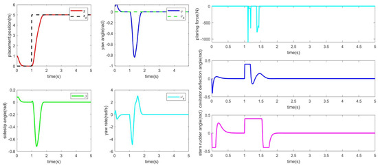
Figure 7. Response curve of the sliding mode variable structure control system for a supercavitating vehicle.

Findings can be seen in Figure 7. The designed control system tracks the desire command, and each state ultimately reaches stability. When the desire command changes sharply, lateral placement tracks the desire command at about 1.8 s. Yaw angle has the greatest value at −0.8 rad at 1.3 s; slide side angle has the greatest value at −0.7 rad at 1.3 s. The yaw rate has two peaks: −4.9 rad/s at 1.2 s and 3 rad/s at 1.5 s. Yaw angle, slide side angle, and yaw rate are all converge to zero at 1.9 s. There is no planing force before the sharp change in expectation command; after the sharp change, the greatest value in planing force is −1098 N; after 1.4 s, the planing force disappears. The deflection angles of the cavitator and fin reach their limit magnitudes at the beginning of the simulation and at about 1 s. After 1 s, the deflection angle of the cavitator lasts 0.2 s, reduces gradually, and stabilizes at 0 at 1.8 s; the stern rudder angle lasts 0.5 s, reduces gradually, and converges to zero at about 2 s.

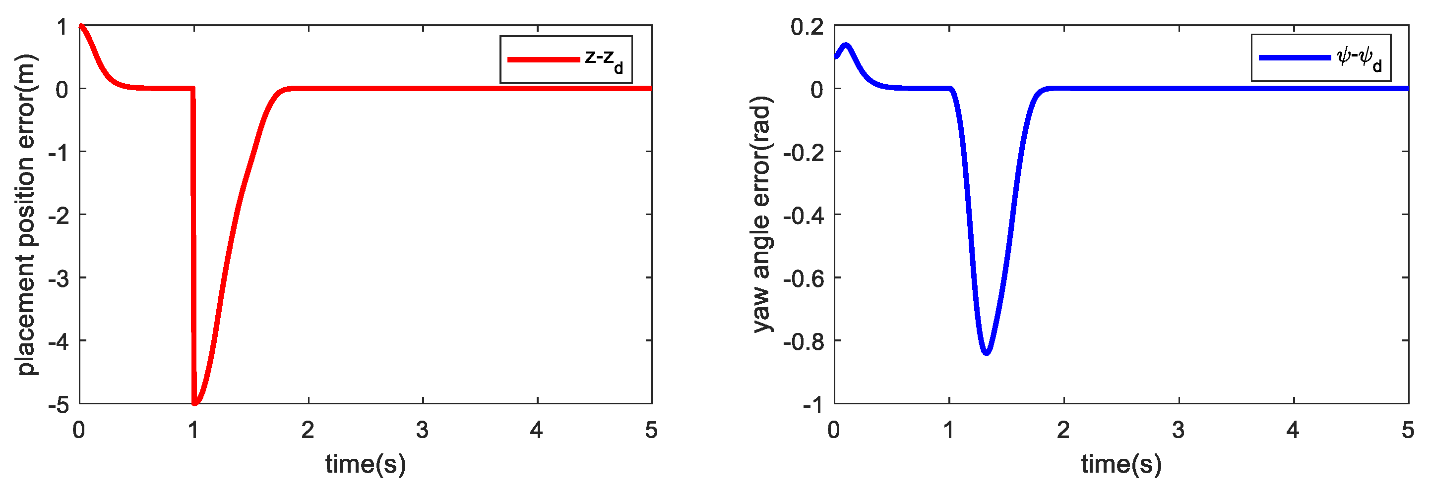
Tracking errors of placement position and yaw angle are shown in Figure 8. We can see that the maximum error of placement position is 5 m and the maximum error of yaw angle is 0.8 rad. The maximum value appears at the instant the command changes and tends toward zero; therefore, the maximum value is acceptable.

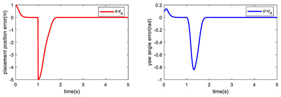
Figure 8. Tracking errors of placement position and yaw angle.

4. Design of a Sliding Mode Variable Structure Controller Based on a Radial Basis Function Neural Network Observer

Assuming that slide side angle rate and yaw rate are unknown signals, a state observer was designed to approximate those signals; as there are uncertainty and unobtained signals in the dynamic model, a radial basis function neural network observer was designed to observe the unknown variable and then, according to the approximated value, to construct a sliding mode variable structure controller to realize trajectory tracking.

4.1. State Observer

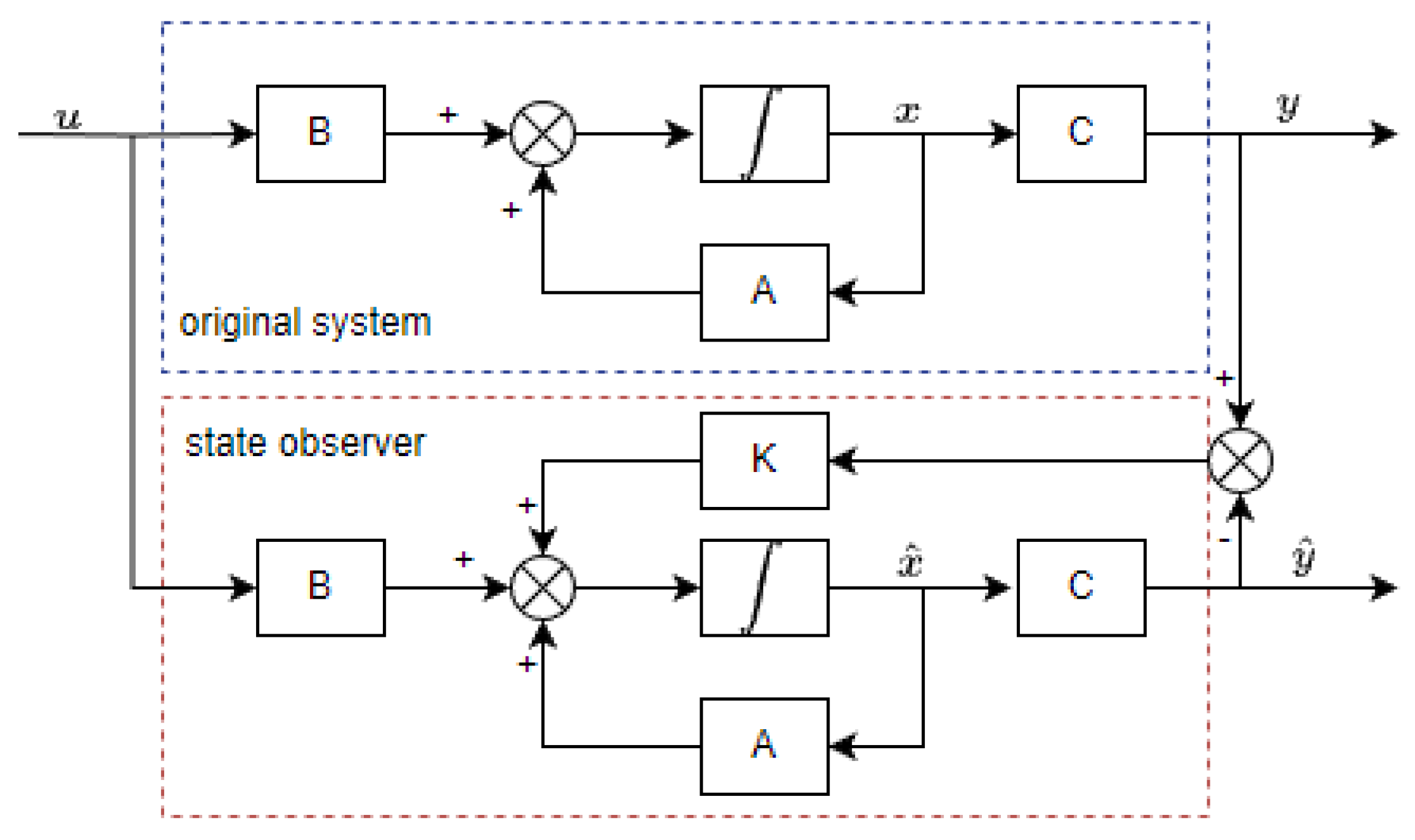
In general, controller design requires that state variables can be measured. However, in actual systems, some variables cannot be obtained directly by sensors. In this situation, the use of a state observer is proposed. A state observer is realized through the system model, that is, the state observer is based on the model of the system, and a new system is reconstructed with the same model as the original system. Output and input are required only to observe the other state of the original system.

In Figure 9 $x$ is state variable, $u$ is the control variable and $y$ is the output of the original system. $\widehat{x}$ is the state variable of the observer, that is, the approximate value of $x$, and $\widehat{y}$ is the output of the state observer, that is, the approximate value of $y$. $K$ is the gain of the state observer.

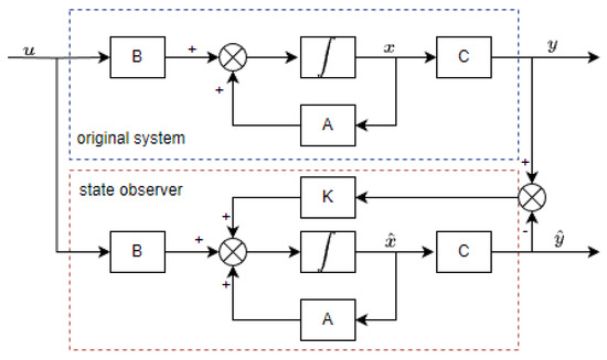
Figure 9. Diagram of the state observer.

The theory of a state observer considers the observed system as follows:

$$\begin{array}{l}\dot{x}=Ax+Bu\\ y=Cx\end{array}$$

(49)

where A is the system matrix, B is the input matrix, C is the output matrix, and state variable x cannot be measured.

The state observer was designed as follows:

$$\begin{array}{l}\dot{\widehat{x}}=A\widehat{x}+Bu+K\left(y-\widehat{y}\right)\\ \widehat{y}=C\widehat{x}\end{array}$$

(50)

The state observer was designed to reconstruct the original system, and the output error is examined to control state error, that is, to reduce the approximate error between the real value and the approximation value.

The error between the real value and approximate value is defined as follows:

$$\tilde{x}=x-\widehat{x}$$

(51)

Take the derivative of (51) to obtain

$$\begin{array}{c}\dot{\tilde{x}}=\dot{x}-\dot{\widehat{x}}=Ax+Bu-A\widehat{x}-Bu-K(y-\widehat{y})\\ =Ax-A\widehat{x}-K(Cx-C\widehat{x})=(A-KC)\tilde{x}\end{array}$$

(52)

Then

$$\tilde{x}=\tilde{x}\left(0\right)e^{{\int }_0^t\left(A-KC\right)dt}$$

(53)

From (53), we know that the eigenvalues of matrix (A-KC) determine whether the error is convergent and how it converges. Therefore, observer gain is designed to make the eigenvalues all negative, that is, matrix (A-KC) is a Hurwitz matrix, which guarantees the error will converge.

4.2. Radial Basis Function Neural Network

There are three layers in a radial basis function neural network: the input layer, the hidden layer, and the output layer. Weights are all equal to 1 from the input layer to hidden layer, that is, the input goes directly to the hidden layer. Each neuron adopts a nonlinear active function—a radial-based function.

A diagram of radial basis function neural network is given in Figure 10.

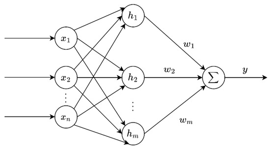
Figure 10. Diagram of a radial basis function neural network.

Where $x={\left[\begin{array}{cccc}{x}_1& x_2& \dots & x_n\end{array}\right]}^T$ expresses the input vector of neural network; $h\left(x\right)=[\begin{array}{cccc}{h}_1(x)& h_2(x)& \dots & h_m(x)\end{array}{]}^T$ is the active function of a neuron of the hidden layer; $w={\left[\begin{array}{cccc}{w}_1& w_2& \dots & w_m\end{array}\right]}^T$ expresses the weight of the output layer; and $y$ is the output of the neural network.

The active function of the hidden layer is as follows:

$$h_j\left(x\right)=\mathit{exp}\left(-{\displaystyle \frac{{‖x-c_j‖}^2}{2b_j^2}}\right),j=\mathrm{1,2},\dots ,m$$

(54)

where $c_j$ expresses the center vector of Gaussian function, $b_j$ is the width of Gaussian function, $\parallel \cdot \parallel$ is the Euclidean distance.

Network output is expressed as a weight function, as follows:

$$y=w^{T}h\left(x\right)$$

(55)

4.3. Design of a Sliding Mode Variable Structure Controller Based on a State Observer

Assuming yaw rate and slide side angle are unknown in the system, as for model (40), then the state observer is designed as follows:

$$\begin{array}{l}{\dot{\widehat{x}}}_1={\widehat{x}}_2+k_1\left(x_1-{\widehat{x}}_1\right)\\ {\dot{\widehat{x}}}_2=A_1{\widehat{x}}_1+A_2{\widehat{x}}_2+Bu+D{F}_{pz}+k_2\left(x_1-{\widehat{x}}_1\right)\end{array}$$

(56)

where $k_1$ and $k_2$ are positive definiteness diagonal matrices.

Defining the expect command of $x_1$ and $x_2$ as $x_{1d}={\left[\begin{array}{cc}{z}_d& {\psi }_d\end{array}\right]}^T$, ${\dot{x}}_{1d}={\left[\begin{array}{cc}{\dot{z}}_d& {\dot{\psi }}_d\end{array}\right]}^T$, the tracking error of $x_1$ and $x_2$ are $e_1={\widehat{x}}_1-x_{1d}$, $e_2={\widehat{x}}_2-{\dot{x}}_{1d}$; first, derive the tracking error, then the following emerges:

$${\dot{e}}_1={\dot{\widehat{x}}}_1-{\dot{x}}_{1d}={\widehat{x}}_2+k_1\left(x_1-{\widehat{x}}_1\right)-{\dot{x}}_{1d}$$

(57)

$${\dot{e}}_2={\dot{\widehat{x}}}_2-{\ddot{x}}_{1d}=A_1{\widehat{x}}_1+A_2{\widehat{x}}_2+Bu+D{F}_{pz}+k_2\left(x_1-{\widehat{x}}_1\right)-{\ddot{x}}_{1d}$$

(58)

Theorem 2.

For system (33), when yaw rate and slide side angle are unknown variables in the system, if and only if the controller is $u=-B^{-1}(c\left({\widehat{x}}_2+k_1\left(x_1-{\widehat{x}}_1\right)-{\dot{x}}_{1d}\right)+A_1{\widehat{x}}_1+A_2{\widehat{x}}_2+D{F}_{pz}+k_2\left(x_1-{\widehat{x}}_1\right)-{\ddot{x}}_{1d}+ks+\eta \mathit{sgn}\left(s\right))$, the system is asymptotic stable.

Proof. 

Design the sliding mode surface as follows:

$$s=c{e}_1+e_2$$

(59)

where $c$ is a positive definite diagonal matrix. □

Take the derivative of the sliding mode surface as follows:

$$\begin{array}{ll}\dot{s}& =c{\dot{e}}_1+{\dot{e}}_2\\ & =c\left({\widehat{x}}_2+k_1\left(x_1-{\widehat{x}}_1\right)-{\dot{x}}_{1d}\right)+A_1{\widehat{x}}_1+A_2{\widehat{x}}_2+Bu+D{F}_{pz}+k_2\left(x_1-{\widehat{x}}_1\right)-{\ddot{x}}_{1d}\end{array}$$

(60)

$$\begin{gathered} u=-B^{-1}(c\left({\widehat{x}}_2+k_1\left(x_1-{\widehat{x}}_1\right)-{\dot{x}}_{1d}\right)+A_1{\widehat{x}}_1+A_2{\widehat{x}}_2+ \\ D{F}_{pz}+k_2\left(x_1-{\widehat{x}}_1\right)-{\ddot{x}}_{1d}+ks+\eta \mathit{sgn}\left(s\right)) \end{gathered}$$

(61)

where $k$ is a positive diagonal matrix, $\eta >0$.

The Lyapunov function for the design is as follows:

$$V={\displaystyle \frac{1}{2}}{s}^{T}s$$

(62)

Taking the derivative of (62), we have the following:

$$\begin{array}{cc}\dot{V}& =s^T\dot{s}=s^T(-ks-\eta \mathrm{sgn}(s))\\ & =-s^{T}ks-s^T\eta \mathrm{sgn}(s)\\ & =-s^{T}ks-\eta \parallel s\parallel \le 0\end{array}$$

(63)

If and only if $s=0$, then $\dot{V}=0$, as for $V\ge 0$, $\dot{V}\le 0$, system is asymptotic stable.

4.4. Design of a Sliding Mode Variable Structure Controller Based on Radial Basis Function Network Observer

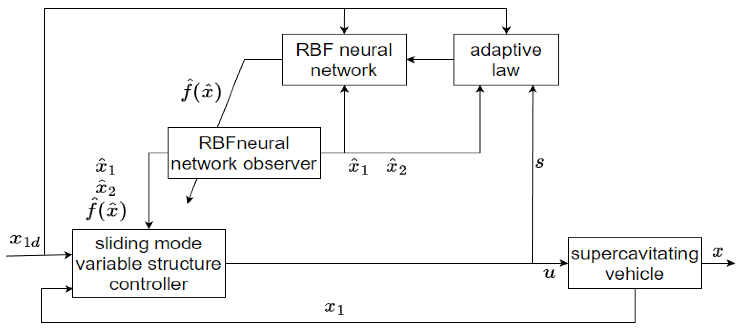
When yaw rate and slide side angle are unknown in the system and there are model uncertainties in the system, a radial basis function neural network observer is designed for the system. The purpose of the observer is to approximate the unknown variable; the purpose of the radial basis function neural network is to approximate model uncertainty. The system diagram is shown in Figure 11.

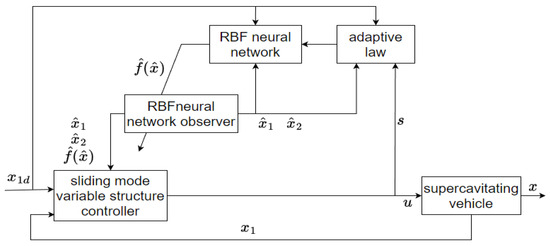
Figure 11. Control system diagram of a radial basis function neural network observer.

Theorem 3.

As for system (33), when yaw rate and slide side angle are unknown and there is model uncertainty in the system, if and only if, controller is $u=-B^{-1}(c\left({\widehat{x}}_2+k_1\left(x_1-{\widehat{x}}_1\right)-{\dot{x}}_{1d}\right)+A_1{\widehat{x}}_1+A_2{\widehat{x}}_2+\widehat{f}\left(\widehat{x}\right)+k_2\left(x_1-{\widehat{x}}_1\right)-{\ddot{x}}_{1d}+ks+\eta \mathit{sgn}\left(s\right))$, the system is asymptotic stable.

Proof. 

As for system (40), the system is transformed into the following form:

$$\begin{array}{l}{\dot{x}}_1=x_2\\ {\dot{x}}_2=A_1{x}_1+A_2{x}_2+Bu+f\left(x,t\right)\end{array}$$

(64)

where $f\left(x,t\right)=D{F}_{pz}+E$ must be approximated by the radial basis function neural network and $E=\Delta A_1{x}_1+\Delta A_2{x}_2+\Delta B_{2}u+d\left(t\right)$ are the total interrupt and uncertainty in the model. □

The design of the the radial basis function neural network observer is as follows [16]:

$$\begin{array}{l}{\dot{\widehat{x}}}_1={\widehat{x}}_2+k_1\left(x_1-{\widehat{x}}_1\right)\\ {\dot{\widehat{x}}}_2=A_1{\widehat{x}}_1+A_2{\widehat{x}}_2+Bu+f\left(x,t\right)+k_2\left(x_1-{\widehat{x}}_1\right)\end{array}$$

(65)

where ${\widehat{x}}_1$ and ${\widehat{x}}_2$ are approximation vectors of $x_1$ and $x_2,k_1$ and $k_2$ are positive diagonal matrices that expresses the gain of the observer. $f\left(x,t\right)$ is unknown; therefore, radial basis function neural network is adopted to approximate it.

A Gaussian function $h\left(x_2\right)$ and idea weight $w^{\mathrm{*}}$ are used to express the approximation value as follows:

$$f^{\ast }\left(\widehat{x}\right)=w^{\ast T}h\left(\widehat{x}\right)$$

(66)

Defining approximation error is $\epsilon$, and assuming the error is bounded, $‖\epsilon ‖\le {\epsilon }_N$, such that:

$$f\left(x,t\right)=w^{\ast T}h\left(\widehat{x}\right)+\epsilon$$

(67)

Let the approximation weight of network is $\widehat{w}$, then, the approximation value of $f\left(x,t\right)$ is $\widehat{f}\left(\widehat{x}\right)$, as follows:

$$\widehat{f}\left(\widehat{x}\right)={\widehat{w}}^{T}h\left(\widehat{x}\right)$$

(68)

Define the weight error as follows:

$$\tilde{w}=\widehat{w}-w^{\ast }$$

(69)

Then, the error between actual value and approximation value is as follows:

$$\begin{array}{ll}f(x,t)-\widehat{f}(\widehat{x})& =\epsilon +w^{\ast T}h(\widehat{x})-{\widehat{w}}^{T}h(\widehat{x})\\ & =\epsilon +\left(w^{{\ast }^T}-{\widehat{w}}^T\right)h(\widehat{x})\\ & =\epsilon -{\tilde{w}}^{T}h(\widehat{x})\end{array}$$

(70)

Define the state variable expect command of $x_1$ and $x_2$ as $x_{1d}={\left[\begin{array}{cc}{z}_d& {\psi }_d\end{array}\right]}^T,{\dot{x}}_{1d}={\left[\begin{array}{cc}{\dot{z}}_d& {\dot{\psi }}_d\end{array}\right]}^T$, the tracking error of variable $x_1$ and $x_2$ is $e_1={\widehat{x}}_1-x_{1d},e_2={\widehat{x}}_2-{\dot{x}}_{1d}$, the tracking error can be derived as:

$${\dot{e}}_1={\dot{\widehat{x}}}_1-{\dot{x}}_{1d}={\widehat{x}}_2+k_1\left(x_1-{\widehat{x}}_1\right)-{\dot{x}}_{1d}$$

(71)

$${\dot{e}}_2={\dot{\widehat{x}}}_2-{\ddot{x}}_{1d}=A_1{\widehat{x}}_1+A_2{\widehat{x}}_2+Bu+f\left(x,t\right)+k_2\left(x_1-{\widehat{x}}_1\right)-{\ddot{x}}_{1d}$$

(72)

Design the sliding mode surface as follows:

$$s=c{e}_1+e_2$$

(73)

where $c$ is the positive dialog matrix.

Take the derivative of the sliding mode surface

$$\begin{array}{ll}\dot{s}& =c{\dot{e}}_1+{\dot{e}}_2\\ & =c\left({\widehat{x}}_2+k_1\left(x_1-{\widehat{x}}_1\right)-{\dot{x}}_{1d}\right)+A_1{\widehat{x}}_1+A_2{\widehat{x}}_2+Bu+f(x,t)+k_2\left(x_1-{\widehat{x}}_1\right)-{\ddot{x}}_{1d}\end{array}$$

(74)

In the design, if the tendency law is $\dot{s}=-ks-\eta \mathit{sgn}\left(s\right)$, the control law is as follows:

$$\begin{gathered} u=-B^{-1}(c\left({\widehat{x}}_2+k_1\left(x_1-{\widehat{x}}_1\right)-{\dot{x}}_{1d}\right)+A_1{\widehat{x}}_1+A_2{\widehat{x}}_2+ \\ \widehat{f}\left(\widehat{x}\right)+k_2\left(x_1-{\widehat{x}}_1\right)-{\ddot{x}}_{1d}+ks+\eta \mathit{sgn}\left(s\right)) \end{gathered}$$

(75)

where $k$ is a positive define diagonal matrix, $\eta \ge {\epsilon }_N>0$.

In the design, the Lyapunov function is as follows:

$$V={\displaystyle \frac{1}{2}}{s}^{T}s+{\displaystyle \frac{1}{2\gamma }}{‖{\tilde{w}}^T‖}^2$$

(76)

Taking the derivative of (76), have

$$\begin{array}{ll}\dot{V}& =s^T\dot{s}+{\displaystyle \frac{1}{\gamma }}\mathrm{tr}\left({\tilde{w}}^T\dot{\tilde{w}}\right)\\ & =s^T(f(x,t)-\widehat{f}(\widehat{x})-ks-\eta \mathrm{sgn}(s))+{\displaystyle \frac{1}{\gamma }}\mathrm{tr}\left({\tilde{w}}^T\dot{\widehat{w}}\right)\\ & =s^T\left(\epsilon -{\tilde{w}}^{T}h(\widehat{x})-ks-\eta \mathrm{s}\mathrm{g}\mathrm{n}(s)\right)+{\displaystyle \frac{1}{\gamma }}\mathrm{tr}\left({\tilde{w}}^T\dot{\widehat{w}}\right)\\ & =-s^{T}ks-s^T\eta \mathrm{sgn}(s)+s^T\epsilon -s^T{\tilde{w}}^{T}h(\widehat{x})+{\displaystyle \frac{1}{\gamma }}\mathrm{tr}\left({\tilde{w}}^T\dot{\widehat{w}}\right)\\ & =-s^{T}ks-s^T\eta \mathrm{sgn}(s)+s^T\epsilon -\mathrm{tr}\left({\tilde{w}}^{T}h(\widehat{x})s^T\right)+{\displaystyle \frac{1}{\gamma }}\mathrm{tr}\left({\tilde{w}}^T\dot{\widehat{w}}\right)\\ & =-s^{T}ks-s^T\eta \mathrm{sgn}(s)+s^T\epsilon +\mathrm{tr}\left({\tilde{w}}^T\left({\displaystyle \frac{1}{\gamma }}\dot{\widehat{w}}-h(\widehat{x})s^T\right)\right)\end{array}$$

(77)

Select an adaptive law as follows:

$$\dot{\widehat{w}}=\gamma h\left(\widehat{x}\right)s^T$$

(78)

Then

$$\dot{V}=-s^{T}ks-s^T\eta \mathit{sgn}\left(s\right)+s^T\epsilon \le 0$$

(79)

For $V\ge 0,\dot{V}\le 0$, therefore, $s$ and $\tilde{w}$ are bounded; when $\dot{V}\equiv 0$, $s=0$; when $t\to \mathrm{\infty }$, $s\to 0$, then $e_1\to 0,e_2\to 0$ and the system is asymptotic stable. In this method, the approximation value is designed by adaptive law, therefore it cannot be guaranteed that $\tilde{w}$ will converge to zero; moreover, there is no guarantee of convergence for $\widehat{f}\left(\widehat{x}\right)$.

5. Simulation Analysis

5.1. Simulation Analysis of a Sliding Mode Variable Structure Controller Based on a State Observer

The simulation interval was set to 5 s; the simulation step was set to a fixed step of 0.01 s; the initial conditions of the simulation were set to $z_0=1,{\dot{z}}_0=-0.5,{\psi }_0=0.1,{\beta }_0={\psi }_0+{\displaystyle \frac{{\dot{z}}_0}{v}},{\omega }_{y0}=0$, with the controller parameters $c=diag\left\{\mathrm{15,15}\right\},k=diag\left\{\mathrm{2,2}\right\},\mathrm{a}\mathrm{n}\mathrm{d} \eta =0.01$. The observer parameter qwas $k_1=diag\left\{\mathrm{5,5}\right\},k_2=diag\left\{\mathrm{5,5}\right\}$. To prevent the deflection angle form exceeding the bound, the limit of the deflection angle of the actuator was set to 0.4 rad and the expect command was set to a value published previously (48).

Simulation curves for each variable and control variable are shown in Figure 12.

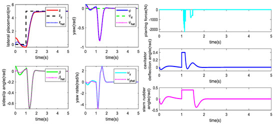
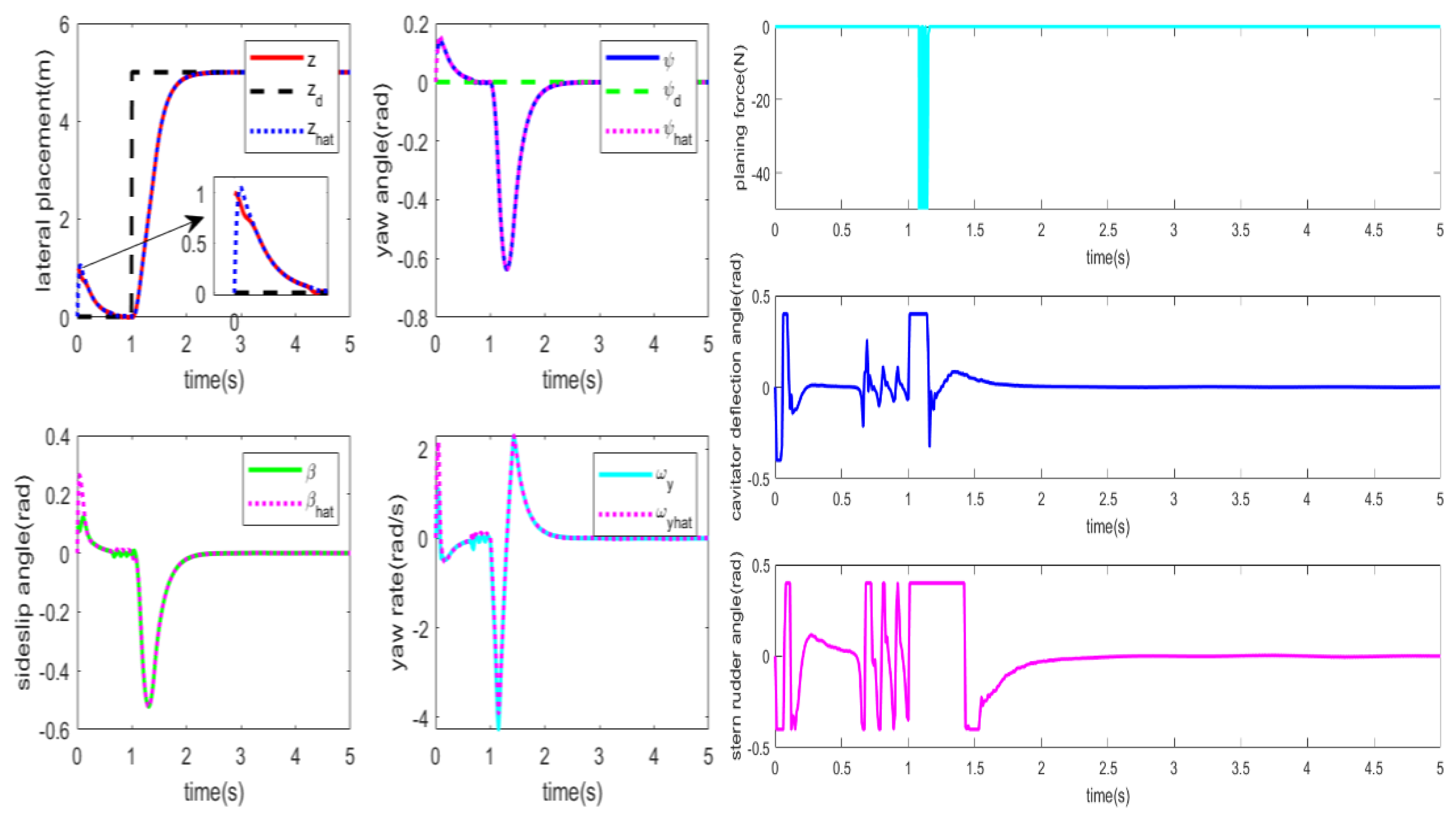
Figure 12. Step-response curves of the state variable, planing force and control input.

As shown in Figure 12, the output signal z_hat of the state observer tracks the actual output signal z of the model at about 1 s; lateral placement z decreases to 0 at 0.47 s and reaches its maximum value of −0.41 m at 1 s; when the expect command z_d changes sharply, the lateral placement z tracks the expect command at about 2.5 s. At the beginning of the simulation, the yaw angle $\psi$ decreases from the initial value; after the changes, at 1.35 s, the maximum value is −0.83 rad, and at about 2.5 s, the yaw angle $\psi$ converges to zero. The slide side angle $\beta$ reaches its maximum value of −0.7 rad at about 1.3 s and converges to zero at about 2.5 s. The yaw rate ${\omega }_y$ changes dramatically: at about 1.2 s, it reaches its negative maximum of −4.74 rad/s at about 1.5 s; it reaches its positive maximum value of 2.78 rad/s, and it is stable at 2.5 s and converges to zero. Planing force, at about 1.1 s, reaches its maximum value of −2250 N; after 1.5 s, there is no planing force measured. The cavitator deflection angle reaches its positive maximum value of 0.4 rad at 1 s; the value remains steady for 1.5 s, and it begins to decrease at about 2 s and tends towards zero. The stern rudder angle reaches its positive bound of 0.4 rad when the command changing sharply and holds this value for 0.5 s, then decreases gently. At about 2 s, it tends towards stability at zero. In summary, lateral placement tracks the step signal, and the other states are also stable.

In the sinusoid signal, the parameters of the controller and observer do not change. The simulation interval is 10 s, and the expect command is set as follows:

$$z_d=5\mathit{sin}\left({\displaystyle \frac{\pi t}{2}}\right), {\psi }_d=-{\displaystyle \frac{{\dot{z}}_d}{v}}$$

(80)

Simulation curves of each state variable and the control input of the supercavitating vehicle are shown in Figure 13.

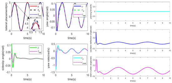
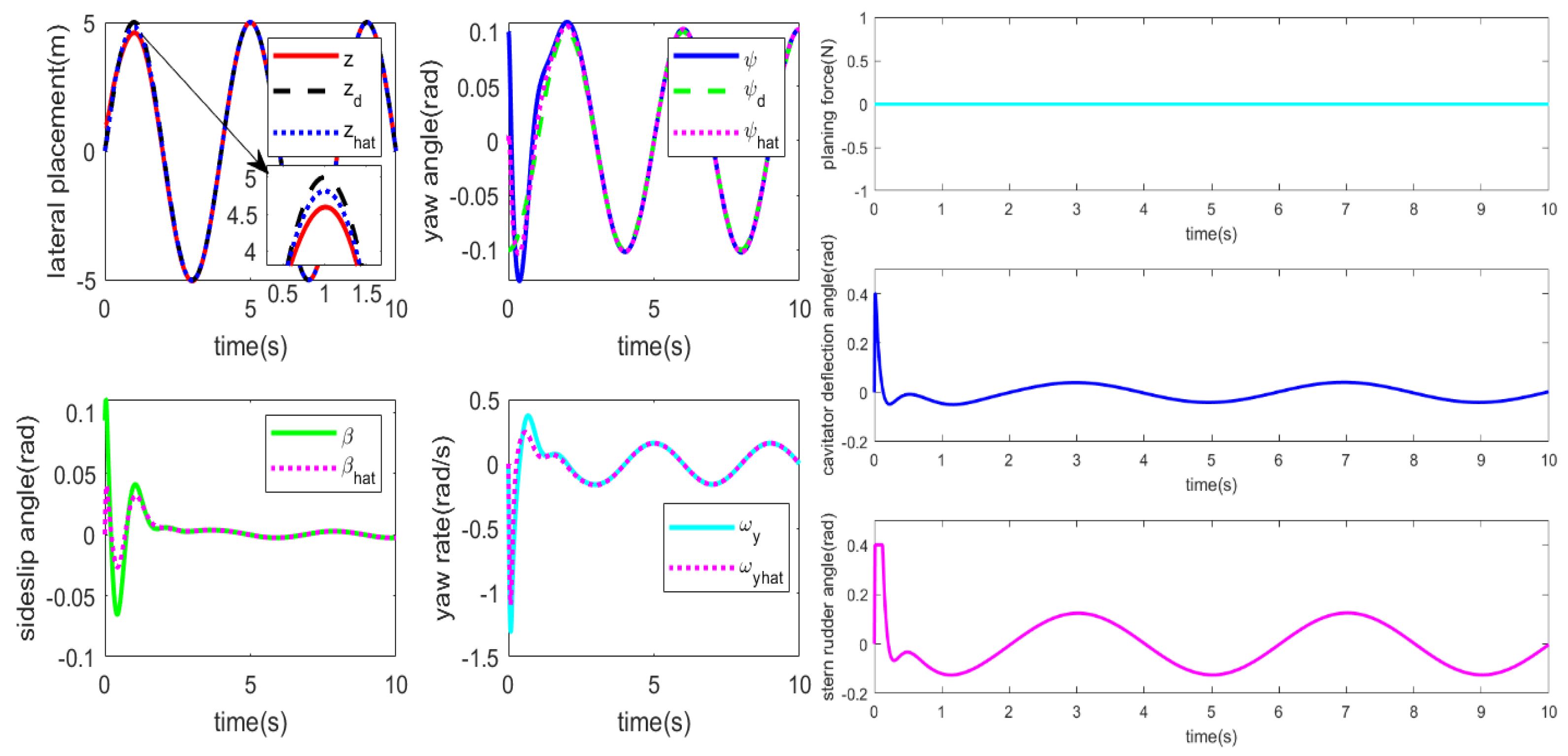
Figure 13. Sinusoid response curves of the vehicle.

As shown in Figure 13, the output signal z_hat of the state observer tracks the output signal z of the actual model at about 2.5 s. The lateral placement z of the actual output of model tracks the expect command z_d at 1.5 s; the yaw angle $\psi$ of the actual output of the model tracks the expect yaw command at 2.5 s; the slide side angle $\beta$ converges to zero at about 2.5 s; the yaw rate ${\omega }_y$ fluctuates in the range of $\pm 0.16$ rad/s after 1.6 s, coinciding with the changing tendency of the yaw angle. During the simulation process, there is no planing force. The deflection angle of the cavitator and stern rudder are large at the beginning of the simulation, and both reach their limits; after 0.1 s, they decrease gradually. After 0.1 s, the deflection angle of the cavitator fluctuates within $\pm 0.04$ rad and the deflection angle of the stern rudder fluctuates within $\pm 0.13$ rad. In summary, the controlled system with an observer tracks the expect command, and the system is stable.

5.2. Simulation Analysis of a Sliding Mode Variable Structure Controller Based on a Radial Basis Function Neural Network Observer

The simulation interval was set to 5 s and the simulation step to a fixed step of 0.01 s, and the initial conditions of the simulation were $z_0=1,{\dot{z}}_0=-0.5,{\psi }_0=0.1,{\beta }_0={\psi }_0+{\displaystyle \frac{{\dot{z}}_0}{v}},{\omega }_{y0}=0$. The controller parameters were $c=diag\left\{\mathrm{100,100}\right\},k=diag\left\{\mathrm{5,5}\right\},\eta =0.01$. The observer parameters were $k_1=diag\left\{\mathrm{50,50}\right\},k_2=diag\left\{\mathrm{1000,1000}\right\}$. The initial weight of the neural network was 0, and the center vector and width of Gaussian function of the radial basis function neural network were as follows:

$$c_R=\left[\begin{array}{ccccccccc}-4& -3& -2& -1& 0& 1& 2& 3& 4\\ -4& -3& -2& -1& 0& 1& 2& 3& 4\\ -4& -3& -2& -1& 0& 1& 2& 3& 4\\ -4& -3& -2& -1& 0& 1& 2& 3& 4\end{array}\right], b_R=0.2$$

(81)

The parameter of adaptive law is $\gamma =500$; a random parameter perturbation of $-20\%~20\%$ was added to the model, and outside interruption was $d\left(t\right)=[\begin{array}{cc}0.2\mathit{sin}(\pi t)& 0.2\mathit{sin}(2\pi t)\end{array}{]}^T$. To prevent the deflection angle from exceeding the limit, the deflection angle of actuator was set to not exceed 0.4 rad and the expect command was set as in Formula (48).

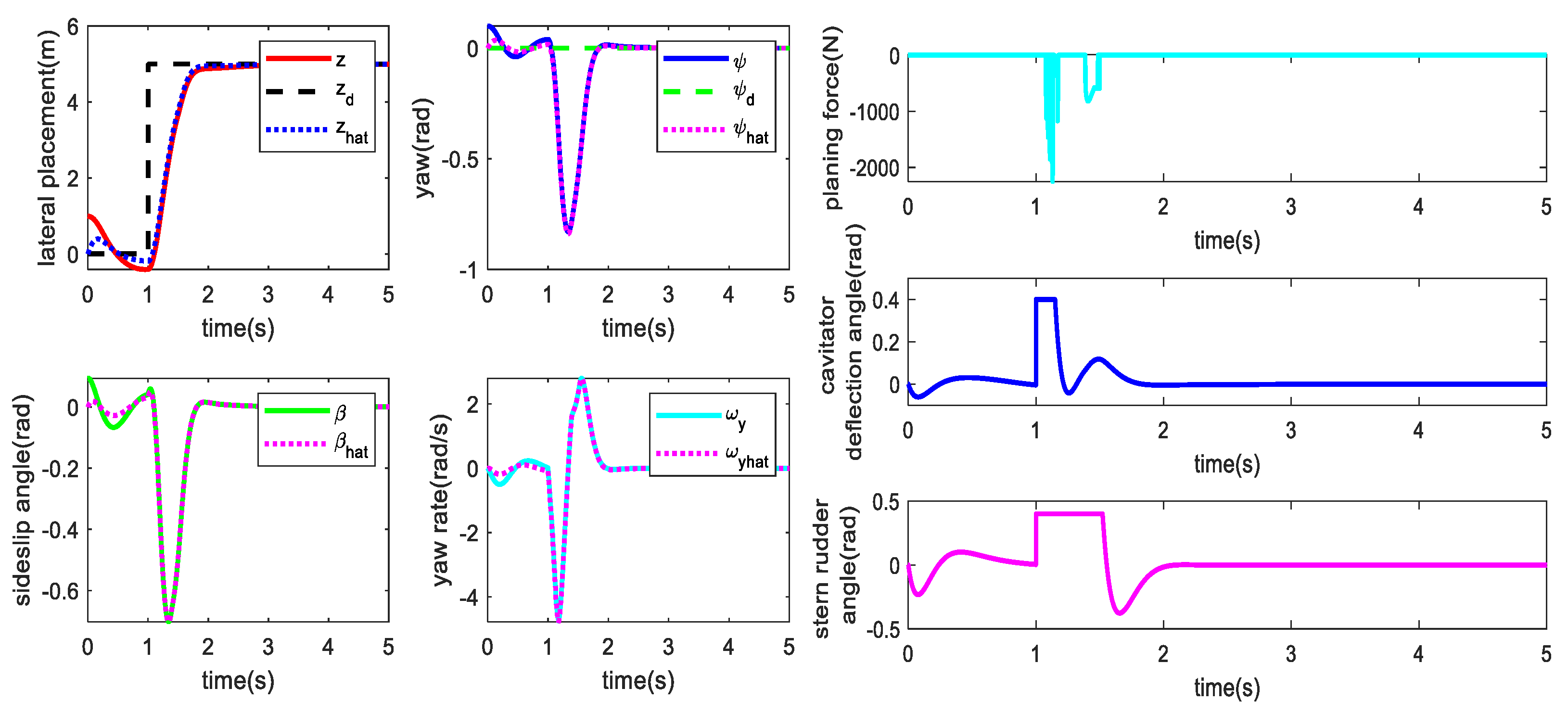
Simulation curves of each state variable and the control input of a supercavitating vehicle are shown in Figure 14.

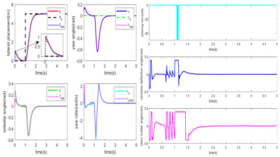
Figure 14. Step-response curves of supercavitating vehicle without parameter perturbation or outside disturbance.

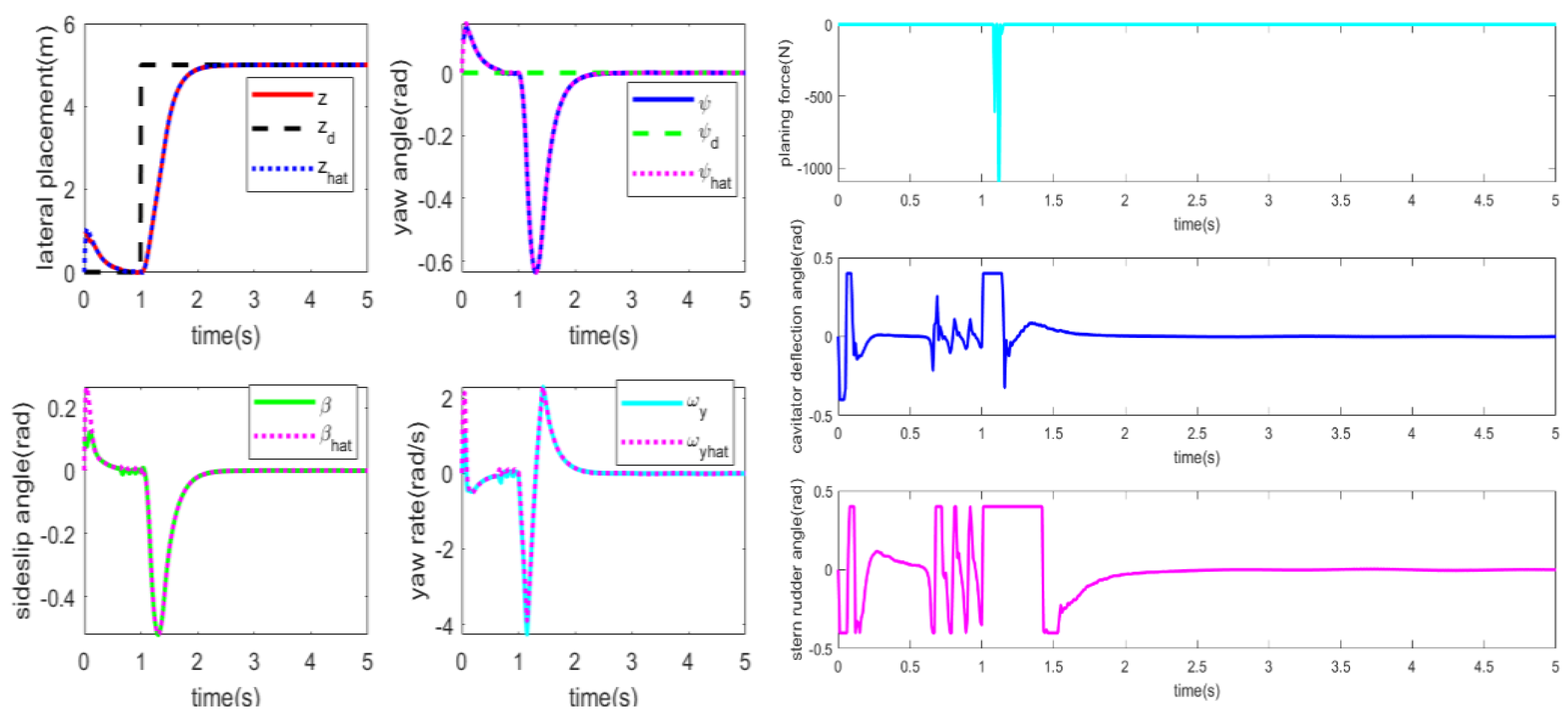
Figure 14 shows curves of each state variable, planing force and control input with no parameter disturbance and no outside interrupt in the model. As shown in Figure 14, the output signal of the observer tracks the actual output signal of the model at the beginning of the simulation. Lateral placement tracks the expect command, and the maximum value of the planing force is just −50 N. The deflection angles of the cavitator and stern rudder converge to zero at about 2.5 s.

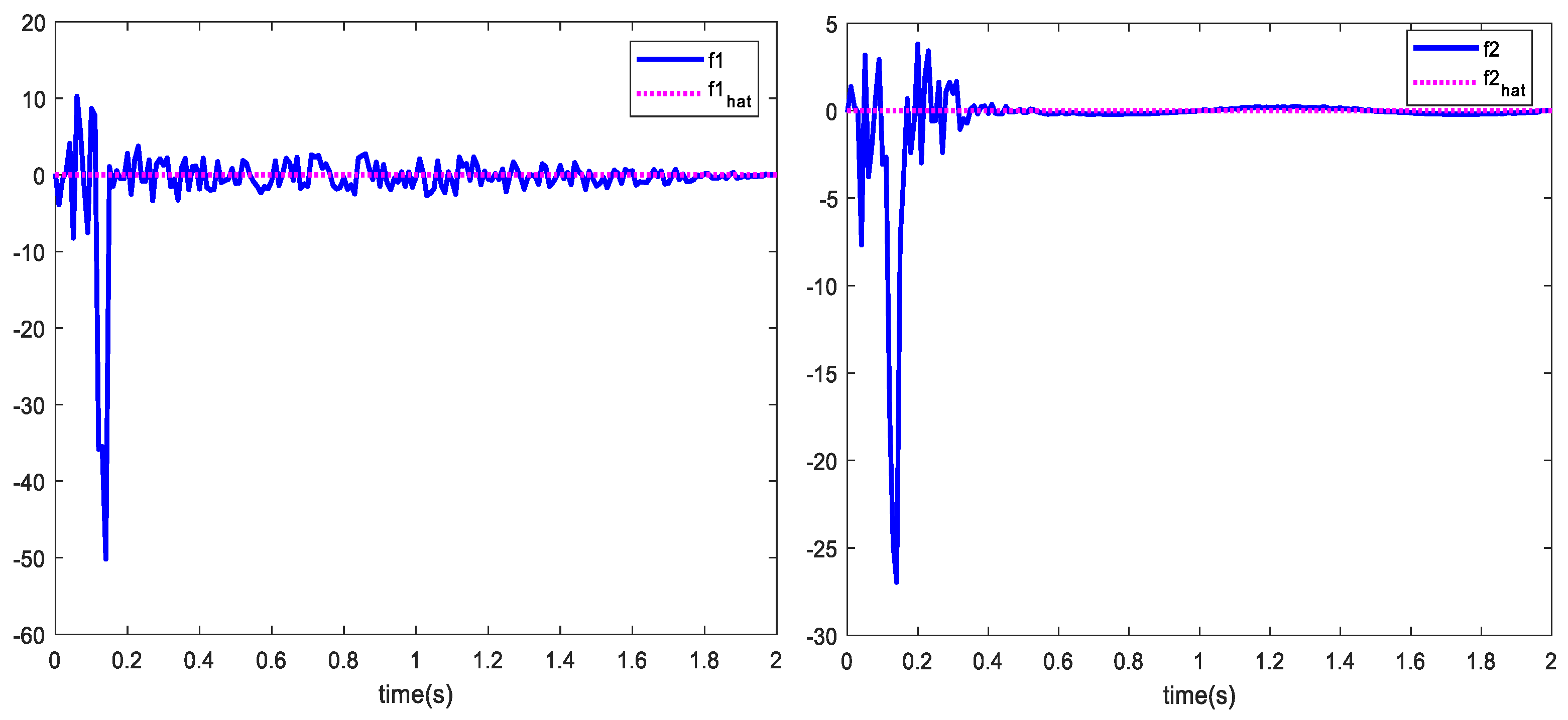
As shown in Figure 15, the lateral placement, yaw angle, slide side angle and yaw rate of the observer track the actual output of model at the beginning of the simulation. The error in yaw rate between the observer and the actual model reaches a large value at 0.05 s and 1.15 s. Before 1 s, although lateral placement, slide side angle and yaw rate maintain their initial values, lateral placement and yaw gradually approach the expect value of zero under the control effect. When the expect lateral placement reaches 5 m, lateral placement tracks the expect command at about 2.4 s, yaw reaches the maximum value of −0.64 rad at 1.3 s and converges to zero at about 2.4 s. Slide side angle reaches the maximum value of −0.52 rad at 1.3 s and converges to zero at about 2.4 s. Yaw rate ${\omega }_y$ changes significantly; it has a negative maximum value of −4.39 rad/s at 1.15 s, and at 1.4 s, it reaches its positive maximum value of 2.31 rad/s; at about 2.4 s, it tends towards stability and converges to zero. At the beginning of the simulation, there is no planing force; after the sharp changes in the command, the planing force emerge. At 1.1 s, it reaches its maximum value of −1105.4 N. After 1.16 s, the planing force disappears. After the command changes, the deflection angle of the cavitator and stern rudder initially oscillate and reaches their limit values frequently. At about 2.4 s, they both converge to stability at zero. Figure 16 represents the approximation result from the observer for the uncertainty part of the model with disturbance. The dashed line represents the approximation results of uncertainty from the neural network; the bold line represents the uncertainty of the actual output of the model. As shown in the figure, because the interrupt is random, the uncertainty of the actual model includes large oscillations, especially at the beginning of the simulation and when the command changes sharply. The approximation of the radial basis function neural network ultimately converges to a stable value.

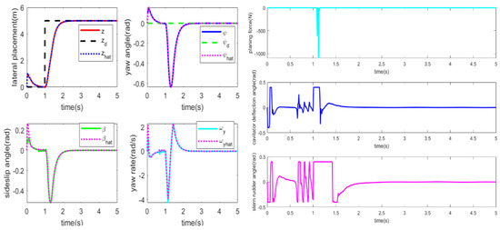
Figure 15. Step-response curves of a supercavitating vehicle (with parameter disturbance and interrupts).

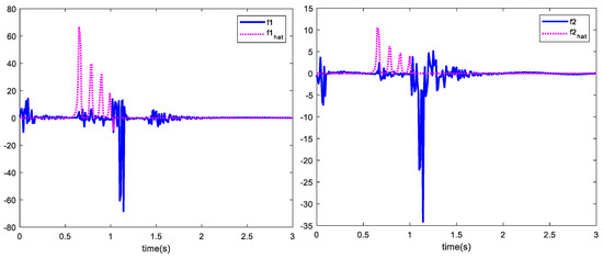
Figure 16. The uncertainty part of the model and its approximation value.

In tracking the sinusoid signal, the parameters of controller and observer do not change: the simulation interval is set to 10 s, the expect command is as in (80), and the curves of each state variable and control input are shown in Figure 17.

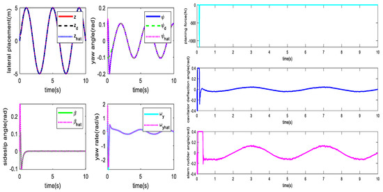
Figure 17. Sinusoid-track response curves of each state variable and planing force and control input.

As shown in Figure 17, the output of the radial basis function neural network observer tracks the actual output at the beginning of the simulation. Lateral placement, yaw angle, slide side angle and yaw rate track the actual output at 0.15 s, 0.15 s,0.1 s, 0.2 s and 0.2 s. Lateral placement tracks the expect command at about 0.9 s, and yaw tracks the expect command at 0.9 s. Slide side angle converges to zero at 1 s, and yaw rate fluctuates between rad/s, coinciding with the tendency. At 0.14 s, a planing force is produced. Its maximum value is −1428.6 N, and the planing force disappears after reaching this value. The deflection angles of the cavitator and stern rudder reach their limit values at the beginning of the simulation, and then the deflection angle of the cavitator and the stern rudder fluctuate within rad. Figure 18 shows that uncertainty created by random parameter disturbance and interrupts has significant effect on the system before 0.5 s. The input of the radial basis function neural network varies widely; thus, the Gaussian function is small, which means that the network weight obtained by adaptive law is very small; then, the output of the radial basis function neural network is small.

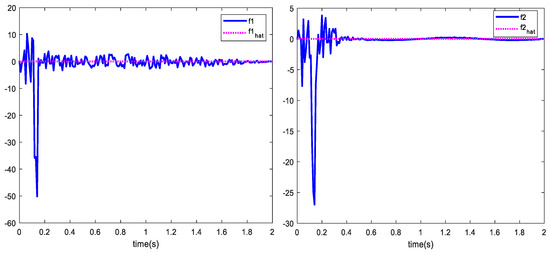
Figure 18. Approximation value of the uncertainty part of the model.

6. Conclusions

Focusing on the lateral movement of a supercavitating vehicle, a mathematical model of lateral movement is established. Because there are unknown state variables and uncertainty in the model, it is difficult to design the controller. To solve these problems, a state observer, radial basis function neural network observer and sliding mode variable structural controller are combined to realize lateral control for a supercavitating vehicle. A state observer is used to approximate unknown variables in the model, while the radial basis function neural network approximates the uncertainty of the model and adaptive law is used to take the approximate-value approach to the actual model. A simulation was conducted to verify that lateral motion was stable. To prevent the deflection angle from exceeding the limit amplitude, the controller limits its amplitude. Simulation results show that the designed observer can approximate the state variable of the original system and that the controller can realize fast trajectory tracking.

The strengths of this paper are as follows: a control system was designed for the lateral motion of a supercavitating vehicle, solving the problem that arises because some states are difficult to measure. However, the lateral model of a supercavitating vehicle includes many assumption conditions, such as the linearization assumption at the benchmark; meanwhile, there are many factors that have not been considered, such as variability in the hydrodynamic coefficients. In future work, the above areas should be the focus of in-depth research.

References

- Logvinovich, G.V. Hydrodynamics of Flows with Free Boundaries; Translated from the Russian, NASA-TF-F-658; U.S. Department of Commerce: Washington, DC, USA, 1972.
- Kirschner, I.; Uhlman, J.; Perkins, J. Overview of high-speed supercavitating vehicle control. In Proceedings of the AIAA Guidance, Navigation, and Control Conference and Exhibit, Keystone, CO, USA, 21–24 August 2006. [Google Scholar]
- Vasin, A.D. The Principle of Independence of the Cavity Sections Expansion (Logvinovich’s Principle) as the Basis for Investigation on Cavitation Flows; Central Aerodynamic Inst (TSAGI) MOSCOW (RUSSIA): Moscow, Russia, 2001. [Google Scholar]
- Goel, A. Robust Control of Supercavitating Vehicles in the Presence of Dynamic and Uncertain Cavity; University of Florida: Gainesville, FL, USA, 2005. [Google Scholar]
- Savchenko, Y.N.; Semenenko, V.N.; Savchenko, G.Y. Peculiarites of Supercavitating Vehicles’ Maneuvering. Int. J. Fluid Mech. Res. 2019, 46, 309–323. [Google Scholar] [CrossRef]
- Semenenko, V.N.; Naumova, Y.I. Study of the supercavitating body dynamics. In Supercavitation: Advances and Perspectives A Collection Dedicated to the 70th Jubilee of Yu; Springer: Berlin/Heidelberg, Germany, 2011; pp. 147–176. [Google Scholar]
- Li, Y.; Wang, C.; Cao, W.; Hou, D.; Zhang, C. Motion characteristics simulations of supercavitating vehicle based on a three-dimensional cavity topology algorithm. Appl. Math. Model. 2023, 115, 691–705. [Google Scholar] [CrossRef]
- Mirzaei, M.; Taghvaei, H. Heading control of a novel finless high-speed supercavitating vehicle with an internal oscillating pendulum. J. Vib. Control 2021, 27, 1765–1777. [Google Scholar] [CrossRef]
- Song, S.H.; Lv, R.; Zhou, J.; Wang, Y.M.; Li, J.C. Maneuver Control Method of Supercavity Vehicle Based on Active Bank-To-Turn. J. Unmanned Undersea Syst. 2019, 27, 607–613. [Google Scholar]
- Luo, K.; Dang, J.; Wang, Y. Course Control of Superspeed Underwater Vehicle. Torpedo Technol. 2009, 17, 54–57. [Google Scholar]
- Gao, Y.; Luo, K.; Duan, P. Research on Direction Control of Superspeed Underwater Vehicle. Comput. Meas. Control 2009, 17, 2001–2003+2009. [Google Scholar]
- Chen, Y.; Luo, K.; Wang, L. Research on roll control of superspeed under water vehicle. Comput. Meas. Control 2009, 17, 129–131. [Google Scholar]
- Bai, T.; Bi, X. Studies on lateral motion control of supercavitating vehicle. In Proceedings of the 2011 Third International Conference on Measuring Technology and Mechatronics Automation, Shanghai, China, 6–7 January 2011; IEEE: Piscataway, NJ, USA, 2011; Volume 3, pp. 377–380. [Google Scholar]
- Dzielski, J.; Kurdila, A. A Benchmark Control Problem for Supercavitating Vehicles and an Initial Investigation of Solutions. J. Vib. Control 2016, 9, 791–804. [Google Scholar] [CrossRef]
- Luo, K.; Li, D.; Huang, C.H. Theoretical Basis of Supercavity Vehicle Technology; Beijing Science Press: Beijing, China, 2016. [Google Scholar]
- Liu, J. RBF Neural Network Adaptive Control and MATLAB Simulation; Tsinghua University Press: Beijing, China, 2018. [Google Scholar]
Disclaimer/Publisher’s Note: The statements, opinions and data contained in all publications are solely those of the individual author(s) and contributor(s) and not of MDPI and/or the editor(s). MDPI and/or the editor(s) disclaim responsibility for any injury to people or property resulting from any ideas, methods, instructions or products referred to in the content. |
© 2025 by the authors. Licensee MDPI, Basel, Switzerland. This article is an open access article distributed under the terms and conditions of the Creative Commons Attribution (CC BY) license (https://creativecommons.org/licenses/by/4.0/).