Accurate In-Motion Initial Heading Alignment for Underwater Robots Using a Basis of the Initial Position-Error Space

Abstract

Accurate initial heading alignment is crucial for autonomous underwater vehicles (AUVs) relying on dead-reckoning (DR) navigation. The multiple GNSS position-based alignment (MGPA) method, using standard point positioning (SPP) GNSS, is an applicable approach in marine environments due to its standalone nature. However, the performance of this method is directly degraded by the inherent error in the initial position, which can be relatively large due to the use of SPP. Therefore, this paper proposes a novel iterative method that estimates and corrects errors in both initial heading and position. The core of the method is a decomposition of the coupled 2D optimization problem into two 1D optimizations by identifying an orthogonal correction basis. The effectiveness of the proposed method is validated through at-sea experiments with an AUV. Experimental results demonstrate that the proposed method corrects the initial position error and achieves improved alignment, enhancing DR navigation accuracy.

1. Introduction

In underwater environments, robots designed for tasks such as marine exploration, military reconnaissance, and search-and-rescue require accurate navigation to operate effectively. This requirement is particularly critical for autonomous underwater vehicles (AUVs) that operate without a tether, as the exchange of external information is intrinsically constrained unless they surface or employ dedicated underwater communication systems such as acoustic modems. Due to the attenuation of electromagnetic signals in water, absolute positioning based on the global navigation satellite system (GNSS) is practically unavailable, and the application of perception sensors such as light detection and ranging (LiDAR) that provide relatively high rate and high precision information is also limited.

For these reasons, underwater robots typically estimate their position and attitude using a strapdown inertial navigation system (SINS), and mitigate errors by integrating auxiliary sensors such as a Doppler velocity log (DVL), magnetometer (digital compass), or depth sensor. Whether based solely on an inertial measurement unit (IMU) or combined with such aiding sensors in an integrated navigation framework, these systems fundamentally rely on dead-reckoning (DR), in which position, velocity and attitude are estimated by integrating measured or derived motion quantities such as acceleration, velocity, or angular rate [1,2,3,4]. However, due to the nature of integration, errors inevitably accumulate over time, causing the estimate to drift. In particular, initial position and attitude errors propagate through all integration steps. Among these, an initial attitude error misaligns the estimated velocity and acceleration vectors at every step, amplifying estimation errors as the number of integration steps increases. Therefore, a precise initial alignment process to estimate accurate initial attitude is crucial in such navigation systems, and a variety of methods have been proposed to address this challenge.

The initial alignment process generally consists of two stages: coarse alignment and fine alignment. The fine alignment is typically implemented using a Kalman filter, which uses the initial attitude estimated from the coarse alignment phase as a prior and refines it through measurement updates [5,6]. The coarse alignment method can be classified into static alignment and in-motion alignment. Static alignment estimates the initial attitude by measuring gravity and the Earth’s rotation rate while the vehicle is stationary. It is suitable when a stable base or long stationary period is feasible. However, most water surface and underwater robots lack a fixed base, are continually affected by currents, and often require rapid deployment or submergence, making static alignment impractical. Consequently, in-motion alignment is predominantly used in field operations [7].

A representative approach for in-motion alignment is the optimization-based alignment (OBA) method first introduced by Wu et al. [8]. This method estimates the initial attitude by exploiting recursive estimation based on multiple observations, and subsequent studies have adapted it for underwater vehicles by integrating DVL measurements [9]. Various improvements have been proposed to enhance the performance of OBA [10,11]. However, it still suffers from slow convergence, particularly in the heading direction, and requires dynamic maneuvers to ensure sufficient observability [8].

To overcome these limitations, multiple studies have used GNSS measurements to improve the initial heading estimation. GNSS-based methods include those that estimate the initial heading using multiple antennas [12,13,14], multiple GNSS-derived velocity vectors [15], or single-antenna GNSS-derived trajectories [16]. In addition, several studies have aligned the DR-derived trajectory with the GNSS-derived trajectory based on their similarity to estimate the initial heading [17,18]. These similarity-based approaches mitigate issues such as comparatively high system cost, structural complexity, and degraded performance at low speeds, which are commonly associated with the aforementioned approaches. However, such methods require that the GNSS-derived trajectory be sufficiently accurate not only because it serves as a ground-truth reference, but also because the travel distance of the DR trajectory is computed from GNSS measurements. Therefore, real-time kinematic (RTK) or time-differenced carrier phase (TDCP) techniques are typically employed to ensure the necessary precision. Such requirements not only limit the applicability of these methods but also make them unsuitable for marine environments, where multipath effects are prevalent during surface operations.

In contrast, some studies have explored the use of GNSS positions computed via standard point positioning (SPP) together with DR positions for initial heading estimation. These methods do not rely on RTK, TDCP, or differential GNSS (DGPS) corrections. Instead, they estimate the initial heading through multiple GNSS positions acquired over a short period (e.g., about 20 s) with the corresponding DR positions computed by the SINS or the integrated underwater navigation system at the same time instances [19,20,21]. By using multiple discrete position samples rather than a single observation, these approaches can maintain a reasonable level of heading estimation accuracy even when high-precision GNSS solutions are unavailable.

However, these multiple GNSS position-based initial heading alignment (MGPA) approaches have their own limitations. The primary issue is that the error in the initial position affects the performance of the initial heading estimation. Typically, this initial position is defined as the first GNSS position acquired during the alignment segment and serves as the starting point for DR. In prior MGPA studies using SPP-based GNSS, which is less reliable, substantial initial position errors can occur. These errors not only lead to inaccurate initial heading estimates but also introduce a persistent position offset into all subsequent DR positions, even if the initial heading is accurately corrected. In contrast, GNSS/DR trajectory-alignment methods using RTK GNSS fundamentally address this issue by employing precise GNSS positioning, thereby minimizing both the magnitude and uncertainty of the initial position error [17]. Meanwhile, studies using TDCP technique address this issue by computing precise position increments rather than relying on absolute positions, making the initial heading estimation independent of the initial position error [15,18]. Similarly, other studies have mitigated the impact of initial position errors by estimating the initial heading using displacement vectors between consecutive GNSS or DR positions, rather than relying on vectors referenced to the absolute initial position [22].

Therefore, this paper proposes an iterative initial position correction method designed to mitigate the adverse effects of the error in GNSS-derived initial position within the MGPA process. The core of the proposed method lies in decomposing the coupled 2D optimization problem. We identify orthogonal correction basis vectors in the initial position-error space from the structure of the alignment problem, which effectively decomposes the horizontal position correction into two 1D optimization problems along two orthogonal directions: along one of which position corrections do not affect the heading estimation, and the other that is coupled with the heading estimation. By iteratively applying corrections along this basis, the algorithm efficiently corrects the error in initial position while simultaneously refining the estimated initial heading.

The main contribution of this work is an improved alignment framework that robustly handles the uncertainties of the GNSS-derived initial position. This leads to improved accuracy in the initial heading estimation and corrects the initial position offset, thereby enhancing the overall accuracy of subsequent DR navigation. To validate the effectiveness of the proposed method, we conducted sea trials with an AUV.

This paper is organized as follows: Section 2 describes the MGPA method and its modified formulation for this study. Section 3 details the proposed iterative initial position correction method. Section 4 demonstrates the sea trials and results. Finally, conclusions are drawn in Section 5.

2. MGPA: Multiple GNSS Position-Based Initial Heading Alignment

An overview of the MGPA approach introduced in prior studies is presented in this section, where the initial heading is estimated by aligning DR positions with the corresponding GNSS positions at matching time instances. The principle and assumptions of MGPA, as well as the procedure for defining GNSS and DR positions within a unified reference frame and estimating the initial heading are described.

2.1. Overview of Multiple GNSS Position-Based Initial Heading Alignment

Figure 1 illustrates the concept of MGPA. The AUV collects GNSS positions and DR positions on the water surface during the alignment process. The DR position is estimated by onboard navigation sensors, while GNSS positions are obtained through SPP. Since the DR position is updated at a much higher rate than GNSS, several DR positions may lie between successive GNSS fixes. Among these the DR positions corresponding to each GNSS epoch are selected for the alignment process.

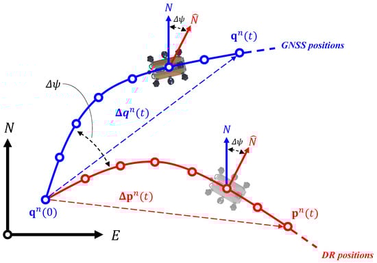
Figure 1. Illustration of the initial heading alignment method using multiple GNSS positions (blue) and DR positions (red). The angle $\mathrm{\Delta }\psi$ represents the offset between magnetic north and true north, corresponding to the initial heading error.

In the underwater robotic platform considered in both prior studies and this work, the navigation system consists of IMU, DVL, digital compass, and depth sensor. The digital compass provides the initial attitude information, where roll and pitch angles can be estimated with relatively high accuracy. However, the heading measured from the compass includes an offset due to the discrepancy between magnetic north and true north. During DR integration, the attitude is updated by gyro measurements, while the linear velocity is estimated by fusing accelerometer and DVL measurements. In addition, the initial position is provided by GNSS. Therefore, the initial heading is estimated by correcting the measurement error of the compass, using the DR positions and the GNSS positions, where this error includes not only measurement noise but also the compass bias.

2.2. Dead Reckoning Position and GNSS Position Computation

In the MGPA, the initial heading is estimated by aligning DR positions with GNSS positions. To estimate the initial heading using these two position sources, both must be expressed in a common coordinate frame. The local navigation frame defined at the initial position is adopted as the common reference. Thus, both positions are transformed and represented with respect to this fixed frame, where the origin corresponds to the first GNSS position.

Under ideal conditions, when the underwater vehicle’s velocity in the body frame (b-frame) and its attitude with respect to the navigation frame (n-frame) are steadily estimated by the SINS, the velocity in the n-frame required for DR can be obtained as:

$${\mathbf{v}}^n={\mathbf{C}}_b^n{\mathbf{v}}^b$$

(1)

where the n-frame follows the North-East-Down (NED) navigation coordinate frame, ${\mathbf{C}}_b^n$ is the direction cosine matrix (DCM) that transforms vectors from the b-frame to the n-frame, and ${\mathbf{v}}^b$ denotes the vehicle’s linear velocity expressed in the b-frame.

The DR position vector can be calculated by integrating the velocity:

$${\mathbf{p}}^n\left(t\right)={\mathbf{p}}^n\left(0\right)+\mathrm{\Delta }{\mathbf{p}}^n\left(t\right)$$

(2)

$$\mathrm{\Delta }{\mathbf{p}}^n\left(t\right)={\int }_0^t{\mathbf{C}}_b^n\left(\tau \right){\mathbf{v}}^b\left(\tau \right)d\tau$$

(3)

where ${\mathbf{p}}^n\left(t\right)$ and ${\mathbf{p}}^n\left(0\right)$ represent the DR position vectors at the current and initial epochs, and $\mathrm{\Delta }{\mathbf{p}}^n={\left[\begin{array}{ccc}\mathrm{\Delta }{p}_N& \mathrm{\Delta }{p}_E& \mathrm{\Delta }{p}_D\end{array}\right]}^T$ represents the position increment vector in the n-frame. The attitude matrix ${\mathbf{C}}_b^n\left(t\right)$ in Equation (3) can be decomposed through the chain rule as:

$${\mathbf{C}}_b^n\left(t\right)={\mathbf{C}}_{b\left(t\right)}^{n\left(t\right)}={\mathbf{C}}_{n\left(0\right)}^{n\left(t\right)}{\mathbf{C}}_{b\left(0\right)}^{n\left(0\right)}{\mathbf{C}}_{b\left(t\right)}^{b\left(0\right)}$$

(4)

Here, ${\mathbf{C}}_{n\left(0\right)}^{n\left(t\right)}$ and ${\mathbf{C}}_{b\left(t\right)}^{b\left(0\right)}$ represent the rotation of the n-frame and b-frame from the initial time to epoch t. ${\mathbf{C}}_{b\left(0\right)}^{n\left(0\right)}$ is the initial attitude matrix of the b-frame with respect to the n-frame. If the alignment process is sufficiently short, the rotation of the navigation frame can be neglected, allowing the following approximation:

$${\mathbf{C}}_{n\left(0\right)}^{n\left(t\right)}\approx {\mathbf{C}}_{n\left(0\right)}^{n\left(0\right)}=\mathbf{I}$$

(5)

where $\mathbf{I}$ is the 3 × 3 identity matrix.

Consequently, DR integration can be performed in the fixed $n\left(0\right)$-frame during the initial heading alignment process, and Equations (2) and (3) can be rewritten as:

$${\mathbf{p}}^{n\left(0\right)}\left(t\right)={\mathbf{p}}^{n\left(0\right)}\left(0\right)+\mathrm{\Delta }{\mathbf{p}}^{n\left(0\right)}\left(t\right)$$

(6)

$$\mathrm{\Delta }{\mathbf{p}}^{n\left(0\right)}\left(t\right)={\int }_0^t{\mathbf{C}}_{b\left(0\right)}^{n\left(0\right)}{\mathbf{C}}_{b\left(\tau \right)}^{b\left(0\right)}{\mathbf{v}}^b\left(\tau \right)d\tau$$

(7)

GNSS measurements provide the vehicle’s latitude $\varphi$, longitude $\lambda$, and altitude h in a geodetic coordinate system (WGS-84). To compare them with DR-derived positions, the GNSS position must also be transformed into the $n\left(0\right)$-frame. For short-range and short-time applications, where the Earth curvature can be locally approximated as planar, the GNSS-derived position increment in the $n\left(0\right)$-frame can be expressed as:

$$\mathrm{\Delta }{\mathbf{q}}^{n\left(0\right)}\left(t\right)=\left[\begin{array}{ccc}{R}_M\left(\varphi \left(0\right)\right)+h\left(0\right)& 0& 0\\ 0& (R_N\left(\varphi \left(0\right)\right)+h\left(0\right))cos\left(\varphi \left(0\right)\right)& 0\\ 0& 0& -1\end{array}\right]\left[\begin{array}{c}\mathrm{\Delta }\varphi \left(t\right)\\ \mathrm{\Delta }\lambda \left(t\right)\\ \mathrm{\Delta }h\left(t\right)\end{array}\right]$$

(8)

$$\mathrm{\Delta }\varphi \left(t\right)=\varphi \left(t\right)-\varphi \left(0\right),\mathrm{\Delta }\lambda \left(t\right)=\lambda \left(t\right)-\lambda \left(0\right),\mathrm{\Delta }h\left(t\right)=h\left(t\right)-h\left(0\right)$$

(9)

The $\mathrm{\Delta }\varphi \left(t\right),\mathrm{\Delta }\lambda \left(t\right),\mathrm{\Delta }h\left(t\right)$ denote the incremental changes in latitude, longitude, and altitude, respectively. The $R_M\left(\varphi \left(0\right)\right)$ and $R_N\left(\varphi \left(0\right)\right)$ represent the radii of curvature of the reference ellipsoid along the meridian and the prime vertical at the initial latitude $\varphi \left(0\right)$ respectively, and are defined as:

$$R_M\left(\varphi \left(0\right)\right)=({\displaystyle \frac{a(1-e^2)}{(1-e^{2}si{n}^2\left(\varphi \left(0\right)\right)}}{)}^{3/2},R_N\left(\varphi \left(0\right)\right)={\displaystyle \frac{a}{\sqrt{1-e^{2}si{n}^2\left(\varphi \left(0\right)\right)}}}$$

(10)

Here, a and e denote the semi-major axis and the first eccentricity of the ellipsoid (WGS-84), respectively.

Consequently, the local GNSS position increment in the $n\left(0\right)$-frame can be equivalently expressed as the difference between the instantaneous and initial positions:

$$\mathrm{\Delta }{\mathbf{q}}^{n\left(0\right)}\left(t\right)={\mathbf{q}}^{n\left(0\right)}\left(t\right)-{\mathbf{q}}^{n\left(0\right)}\left(0\right)$$

(11)

2.3. Initial Heading Estimation

The position equations expressed in the initial position navigation frame in Section 2.2 hold under ideal conditions. However, the estimated motion of the vehicle contains errors that originate from sensor measurements. From Equation (3), the attitude increment term ${\mathbf{C}}_{b\left(t\right)}^{b\left(0\right)}$ is obtained by integrating the angular velocity measured by gyroscopes. In short-duration alignment, these gyro integration errors are relatively small and can be neglected compared to errors in the initial attitude and velocity estimation. For the initial attitude matrix ${\mathbf{C}}_{b\left(0\right)}^{n\left(0\right)}$, as discussed in Section 2.1, when the digital compass is used, roll and pitch can be estimated with relatively high accuracy. Therefore, only the heading error needs to be considered. To reflect these errors, the DR position increment can be expressed as:

$$\mathrm{\Delta }{\widehat{\mathbf{p}}}^{n\left(0\right)}\left(t\right)={\int }_0^t{\widehat{\mathbf{C}}}_{b\left(0\right)}^{n\left(0\right)}{\mathbf{C}}_{b\left(\tau \right)}^{b\left(0\right)}{\widehat{\mathbf{v}}}^b\left(\tau \right)d\tau$$

(12)

$${\widehat{\mathbf{v}}}^b\left(t\right)={\mathbf{v}}^b\left(t\right)+{\mathbf{v}}_e\left(t\right)$$

(13)

where the hat symbol ^ denotes the variables that include measurement errors, and the subscript e represents the corresponding error component.

The initial attitude matrix with errors ${\widehat{\mathbf{C}}}_{b\left(0\right)}^{n\left(0\right)}$ can be written as:

$${\widehat{\mathbf{C}}}_{b\left(0\right)}^{n\left(0\right)}={\mathbf{C}}_{n\left(0\right)}^{n_e\left(0\right)}{\mathbf{C}}_{b\left(0\right)}^{n\left(0\right)}$$

(14)

Here, ${\mathbf{C}}_{n\left(0\right)}^{n_e\left(0\right)}$ denotes the rotation matrix corresponding to the initial heading error $\mathrm{\Delta }{\psi }_e$, which can be expressed as:

$${\mathbf{C}}_{n\left(0\right)}^{n_e\left(0\right)}=\left[\begin{array}{ccc}cos\left(\mathrm{\Delta }{\psi }_e\right)& -sin\left(\mathrm{\Delta }{\psi }_e\right)& 0\\ sin\left(\mathrm{\Delta }{\psi }_e\right)& cos\left(\mathrm{\Delta }{\psi }_e\right)& 0\\ 0& 0& 1\end{array}\right]$$

(15)

Similarly, the GNSS position increment containing measurement errors can be written as:

$$\mathrm{\Delta }{\widehat{\mathbf{q}}}^{n\left(0\right)}\left(t\right)={\widehat{\mathbf{q}}}^{n\left(0\right)}\left(t\right)-{\widehat{\mathbf{q}}}^{n\left(0\right)}\left(0\right)$$

(16)

$${\widehat{\mathbf{q}}}^{n\left(0\right)}\left(t\right)={\mathbf{q}}^{n\left(0\right)}\left(t\right)+{\mathbf{q}}_e\left(t\right)$$

(17)

Since heading estimation in MGPA is performed based on spatial relationship between multiple GNSS-DR position pairs, the initial heading misalignment primarily affects the horizontal motion. Therefore, the quantities of interest are the horizontal position increments. The 3D position increment vectors can be reduced to their horizontal components as:

$$\mathrm{\Delta }{\widehat{\mathbf{p}}}_H\left(t\right)=\left[\begin{array}{c}\mathrm{\Delta }{\widehat{p}}_N^{n\left(0\right)}\left(t\right)\\ \mathrm{\Delta }{\widehat{p}}_E^{n\left(0\right)}\left(t\right)\end{array}\right],\mathrm{\Delta }{\widehat{\mathbf{q}}}_H\left(t\right)=\left[\begin{array}{c}\mathrm{\Delta }{\widehat{q}}_N^{n\left(0\right)}\left(t\right)\\ \mathrm{\Delta }{\widehat{q}}_E^{n\left(0\right)}\left(t\right)\end{array}\right]$$

(18)

For notational convenience, the horizontal position increments of DR and GNSS over N epochs are collectively represented in stacked matrix form as:

$$\mathrm{\Delta }{\widehat{\mathbf{P}}}_H=\left[\begin{array}{c}\mathrm{\Delta }{\widehat{\mathbf{p}}}_H{\left(1\right)}^T\\ \mathrm{\Delta }{\widehat{\mathbf{p}}}_H{\left(2\right)}^T\\ ⋮\\ \mathrm{\Delta }{\widehat{\mathbf{p}}}_H{\left(N\right)}^T\end{array}\right],\mathrm{\Delta }{\widehat{\mathbf{Q}}}_H=\left[\begin{array}{c}\mathrm{\Delta }{\widehat{\mathbf{q}}}_H{\left(1\right)}^T\\ \mathrm{\Delta }{\widehat{\mathbf{q}}}_H{\left(2\right)}^T\\ ⋮\\ \mathrm{\Delta }{\widehat{\mathbf{q}}}_H{\left(N\right)}^T\end{array}\right]$$

(19)

Each row corresponds to the horizontal increment between the initial and each epoch in the same $n\left(0\right)$-frame.

In prior MGPA studies, the horizontal position increments described above have been used to estimate the initial heading by averaging-type approaches. Various implementations of this approach have been adopted, including weighted circular means and Wiener-filter-based formulations. These methods exploit the fact that the compared position pairs contain measurement noise that can be modeled by certain statistical distributions (e.g., Gaussian distributions). By combining multiple observations, the overall estimate benefits from a noise-averaging effect, thereby improving the reliability of the estimated heading. Among these implementations, the following linear least-squares formulation of the same estimation objective is adopted, which preserves the averaging property of prior approaches while providing an analytically tractable cost function that is compatible with the subsequent optimization process. Consequently, the initial heading correction value can be estimated as:

$$\mathrm{\Delta }{\widehat{\psi }}^{*}=arg\underset{\mathrm{\Delta }\widehat{\psi }}{min}\mathcal{J}\left(\mathrm{\Delta }\widehat{\psi }\right)$$

(20)

$$\mathcal{J}\left(\mathrm{\Delta }\widehat{\psi }\right)=\sum _{k=1}^N{\parallel R_H\left(\mathrm{\Delta }\widehat{\psi }\right)\mathrm{\Delta }{\widehat{\mathbf{p}}}_H\left(k\right)-\mathrm{\Delta }{\widehat{\mathbf{q}}}_H\left(k\right)\parallel }^2$$

(21)

where $R_H\left(\mathrm{\Delta }\widehat{\psi }\right)$ denotes the horizontal rotation matrix corresponding to the heading correction angle $\mathrm{\Delta }\widehat{\psi }$. This least-squares formulation yields the statistical averaging effect in a linearized structure that is suitable for integration of initial position correction will be introduced in Section 3.

The closed-form solution for the correction angle estimation can be derived as follows:

$$\mathbf{S}=\mathrm{\Delta }{\widehat{\mathbf{Q}}}_H^T\mathrm{\Delta }{\widehat{\mathbf{P}}}_H=\left[\begin{array}{cc}{s}_{11}& s_{12}\\ s_{21}& s_{22}\end{array}\right]$$

(22)

$$a:=s_{22}+s_{11},b:=s_{21}-s_{12}$$

(23)

$$\mathrm{\Delta }{\widehat{\psi }}^{*}=atan2(b,a)$$

(24)

Here, the estimated correction angle $\mathrm{\Delta }{\widehat{\psi }}^{*}$ exhibits nearly the same magnitude as the initial heading error $\mathrm{\Delta }{\psi }_e$ but with the opposite sign. Applying this correction yields a corrected initial heading close to the true values. For brevity, we refer to this procedure as initial heading estimation in the remainder of the paper.

3. Initial Position Correction Method

3.1. Impact of Initial Position Error on Heading Alignment

To demonstrate the influence of the initial position error on the MGPA process, a simplified conceptual condition is considered, as shown in Figure 2. Although this scenario does not represent an actual navigation situation, it enables clear observation of the effects of errors in initial heading and position by excluding other uncertainty sources. In this simplified condition, the vehicle is assumed to move in a straight line without rotation, and two cases are considered: one with only an initial heading error, and the other with both an initial heading and position error included.

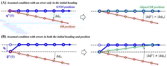
Figure 2. Conceptual illustration of the MGPA alignment result under different initial error conditions. (A) Assumed condition with an error only in the initial heading. (B) Assumed condition with errors in both the initial heading and position.

When only the initial heading error exists, as in Figure 2A, the MGPA estimates a heading correction angle with a same magnitude as the true heading error through the optimization process (24). Using this correction angle, the DR trajectory can be aligned so that it becomes geometrically consistent with the GNSS trajectory. However, when an initial position error is also present, as shown in Figure 2B, the least-square residual minimization yields a correction angle different from the true one, resulting in a misalignment between the two trajectories.

This angular difference depends on the direction of the error in initial position on the horizontal plane. As illustrated in Figure 3, when the initial position error lies in a specific direction, particularly along the GNSS trajectory as in Figure 3B, the estimated correction angle becomes identical in magnitude to the true heading error, even though a position offset exists.

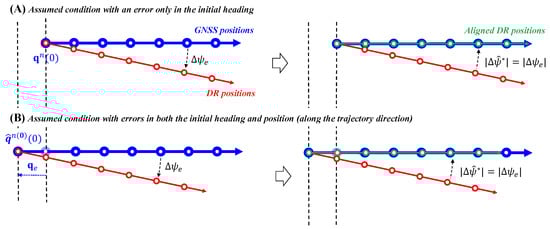
Figure 3. Conceptual illustration of the MGPA alignment result under different initial error conditions. (A) Assumed condition with an error only in the initial heading. (B) Assumed condition with errors in both the initial heading and position, where the position error lies along the trajectory direction.

This directional property provides the key insight for the methodology proposed in the next section: a methodology that identifies an orthogonal basis in order to efficiently correct the error in initial position.

3.2. Identification of an Orthogonal Basis for Initial Position Correction

The error in initial position that affects the estimation of the initial heading exists primarily in the horizontal plane, and correcting it requires estimating two independent variables, constituting a 2D optimization problem. In addition, the heading estimation varies depending on the corrected initial position, making the problem even more complex. In other words, the initial position correction and heading estimation are interdependent and inherently coupled.

However, as described in the previous section, the influence of the error in the initial position on the alignment depends on the direction of the error. In particular, there is a direction along which the error does not affect the heading estimation. Therefore, a direction for correction that does not change the heading estimation can be defined, and the orthogonal direction to it can be regarded as having the greatest influence on the heading estimation. For clarity, these two orthogonal directions are, respectively, referred to as the heading-insensitive direction and the heading-sensitive direction in the following sections. From Equations (12) and (16), it can be seen that among the horizontal position increment vectors used for heading estimation, the initial position error is included only in the GNSS-derived increment. Therefore, when a unit correction vector $\mathbf{u}={\left[\begin{array}{cc}{u}_N& u_E\end{array}\right]}^T$ that represents the heading-insensitive direction is added to correct the initial position error contained in $\mathrm{\Delta }{\widehat{\mathbf{q}}}_H$, the heading correction estimation can be formulated as:

$$\mathrm{\Delta }{\widehat{\psi }}_{\mathbf{u}}^{*}=arg\underset{\mathrm{\Delta }\widehat{\psi }}{min}{\mathcal{J}}_{\mathbf{u}}(\mathrm{\Delta }\widehat{\psi },\mathbf{u})$$

(25)

$${\mathcal{J}}_{\mathbf{u}}(\mathrm{\Delta }\widehat{\psi },\mathbf{u})=\sum _{k=1}^N{\parallel R_H\left(\mathrm{\Delta }\widehat{\psi }\right)\mathrm{\Delta }{\widehat{\mathbf{p}}}_H\left(k\right)-(\mathrm{\Delta }{\widehat{\mathbf{q}}}_H\left(k\right)+\mathbf{u})\parallel }^2$$

(26)

Here, the correction vector is assumed to be defined so that it preserves the same heading estimation as that obtained from the uncorrected case, and must therefore satisfy the following equality constraint, which ensures that the introduction of the correction vector does not change the optimized heading solution:

$$\mathrm{\Delta }{\widehat{\psi }}^{*}=\mathrm{\Delta }{\widehat{\psi }}_{\mathbf{u}}^{*}$$

(27)

Under this equality constraint, the correction vector can be analytically determined. To do this, the horizontal cross-covariance matrix $\mathbf{Z}$ between the DR and GNSS increments (including the correction term $\mathbf{u}$), which is used to compute $\mathrm{\Delta }{\widehat{\psi }}_{\mathbf{u}}^{*}$ is expressed as:

$$\mathbf{Z}={(\mathrm{\Delta }{\widehat{\mathbf{Q}}}_H+{\mathbf{1}}_{N\times 1}{\mathbf{u}}^T)}^T\mathrm{\Delta }{\widehat{\mathbf{P}}}_H=\left[\begin{array}{cc}{z}_{11}& z_{12}\\ z_{21}& z_{22}\end{array}\right]$$

(28)

To satisfy the equality constraint, the elements of the matrix $\mathbf{Z}$ must satisfy the following relationship:

$${\displaystyle \frac{b}{a}}={\displaystyle \frac{z_{21}-z_{12}}{z_{22}+z_{11}}}$$

(29)

This condition implies that the same geometric relationship between the DR and GNSS horizontal increments, as defined in the matrix $\mathbf{S}$, is preserved after applying the correction.

By expanding this in terms of the position correction vector, it can be rewritten as:

$${\displaystyle \frac{b}{a}}={\displaystyle \frac{b+u_E\sum \mathrm{\Delta }{\widehat{p}}_N^{n\left(0\right)}-u_N\sum \mathrm{\Delta }{\widehat{p}}_E^{n\left(0\right)}}{a+u_E\sum \mathrm{\Delta }{\widehat{p}}_E^{n\left(0\right)}+u_N\sum \mathrm{\Delta }{\widehat{p}}_N^{n\left(0\right)}}}$$

(30)

Here, $\sum \mathrm{\Delta }{\widehat{p}}_N^{n\left(0\right)}$ and $\sum \mathrm{\Delta }{\widehat{p}}_E^{n\left(0\right)}$ represent the sum of North and East components of DR-position increments.

By rearranging Equation (30) to solve for the components of $\mathbf{u}$, we obtain the closed-form solution for the unit position correction vector:

$$\mathbf{u}={\displaystyle \frac{\mathit{\alpha }}{\parallel \mathit{\alpha }\parallel }},\mathit{\alpha }:=\left[\begin{array}{c}a\sum \mathrm{\Delta }{\widehat{p}}_N^{n\left(0\right)}-b\sum \mathrm{\Delta }{\widehat{p}}_E^{n\left(0\right)}\\ b\sum \mathrm{\Delta }{\widehat{p}}_N^{n\left(0\right)}+a\sum \mathrm{\Delta }{\widehat{p}}_E^{n\left(0\right)}\end{array}\right]$$

(31)

The unit vector $\mathbf{u}$ therefore represents the heading-insensitive direction. Then, the heading-sensitive direction is orthogonal to $\mathbf{u}$. Consequently, the unit vector representing this direction $\mathbf{n}$ can be defined as:

$$\mathbf{n}=\left[\begin{array}{cc}0& -1\\ 1& 0\end{array}\right]\mathbf{u}$$

(32)

As a result, $\mathbf{u}$ and $\mathbf{n}$ form an orthogonal basis in the horizontal plane. This basis enables a structured approach to correct the error in the initial position efficiently.

3.3. Iterative Process for Initial Position Correction

Based on the orthogonal correction basis vectors defined in Section 3.2, the initial position correction is performed iteratively along the two directions. At each iteration i, the correction is first applied along ${\mathbf{u}}^i$. The optimization problem can be expressed as:

$$\mathrm{\Delta }{\widehat{\psi }}_{{\mathbf{u}}^i}^{*},{\gamma }_{{\mathbf{u}}^i}^{*}=arg\underset{\mathrm{\Delta }{\widehat{\psi }}_{{\mathbf{u}}^i},{\gamma }_{{\mathbf{u}}^i}}{min}{\mathcal{F}}_{{\mathbf{u}}^i}(\mathrm{\Delta }{\widehat{\psi }}_{{\mathbf{u}}^i},{\gamma }_{{\mathbf{u}}^i})$$

(33)

$${\mathcal{F}}_{{\mathbf{u}}^i}(\mathrm{\Delta }{\widehat{\psi }}_{{\mathbf{u}}^i},{\gamma }_{{\mathbf{u}}^i})=\sum _{k=1}^N{\parallel R_H\left(\mathrm{\Delta }{\widehat{\psi }}_{{\mathbf{u}}^i}\right)\mathrm{\Delta }{\widehat{\mathbf{p}}}_H\left(k\right)-(\mathrm{\Delta }{\widehat{\mathbf{q}}}_H^i\left(k\right)+{\gamma }_{{\mathbf{u}}^i}{\mathbf{u}}^i)\parallel }^2$$

(34)

Here, $\mathrm{\Delta }{\widehat{\mathbf{q}}}_H^i$ denotes the GNSS horizontal increment at iteration i, and ${\gamma }_{{\mathbf{u}}^i}$ represents the correction magnitude applied along ${\mathbf{u}}^i$. Since ${\mathbf{u}}^i$ is the heading-insensitive direction, the optimization can be separated into two independent steps:

$$\mathrm{\Delta }{\widehat{\psi }}_{{\mathbf{u}}^i}^{*}=arg\underset{\mathrm{\Delta }{\widehat{\psi }}_{{\mathbf{u}}^i}}{min}{\mathcal{F}}_{{\mathbf{u}}^i}(\mathrm{\Delta }{\widehat{\psi }}_{{\mathbf{u}}^i},0)$$

(35)

$${\gamma }_{{\mathbf{u}}^i}^{*}=arg\underset{{\gamma }_{{\mathbf{u}}^i}}{min}{\mathcal{F}}_{{\mathbf{u}}^i}(\mathrm{\Delta }{\widehat{\psi }}_{{\mathbf{u}}^i}^{*},{\gamma }_{{\mathbf{u}}^i})$$

(36)

The optimal correction magnitude ${\gamma }_{{\mathbf{u}}_i}^{*}$ can be obtained in closed-form as:

$${\gamma }_{{\mathbf{u}}_i}^{*}={\displaystyle \frac{{(R_H\left(\mathrm{\Delta }{\widehat{\psi }}_{{\mathbf{u}}^i}^{*}\right)\sum \mathrm{\Delta }{\widehat{\mathbf{p}}}_H-\sum \mathrm{\Delta }{\widehat{\mathbf{q}}}_H^i)}^T}{N}}{\mathbf{u}}^i$$

(37)

The terms $\sum \mathrm{\Delta }{\widehat{\mathbf{p}}}_H$ and $\sum \mathrm{\Delta }{\widehat{\mathbf{q}}}_H^i$ represent the summed DR-position and GNSS-position increment vectors, respectively. After the correction along ${\mathbf{u}}^i$, the next step applies the correction along the heading-sensitive direction ${\mathbf{n}}^i$:

$$\mathrm{\Delta }{\widehat{\psi }}_{{\mathbf{n}}^i}^{*},{\gamma }_{{\mathbf{n}}^i}^{*}=arg\underset{\mathrm{\Delta }{\widehat{\psi }}_{{\mathbf{n}}^i},{\gamma }_{{\mathbf{n}}^i}}{min}{\mathcal{F}}_{{\mathbf{n}}^i}(\mathrm{\Delta }{\widehat{\psi }}_{{\mathbf{n}}^i},{\gamma }_{{\mathbf{n}}^i})$$

(38)

$${\mathcal{F}}_{{\mathbf{n}}^i}(\mathrm{\Delta }{\widehat{\psi }}_{{\mathbf{n}}^i},{\gamma }_{{\mathbf{n}}^i})=\sum _{k=1}^N{\parallel R_H\left(\mathrm{\Delta }{\widehat{\psi }}_{{\mathbf{n}}^i}\right)\mathrm{\Delta }{\widehat{\mathbf{p}}}_H\left(k\right)-(\mathrm{\Delta }{\widehat{\mathbf{q}}}_H^i\left(k\right)+{\gamma }_{{\mathbf{u}}^i}^{*}{\mathbf{u}}^i+{\gamma }_{{\mathbf{n}}^i}{\mathbf{n}}^i)\parallel }^2$$

(39)

Unlike the correction along ${\mathbf{u}}^i$, this optimization cannot be solved in a simple closed-form. This is because the correction magnitude ${\gamma }_{{\mathbf{n}}^i}$ and the heading correction angle $\mathrm{\Delta }{\widehat{\psi }}_{{\mathbf{n}}^i}$ are inherently coupled. However, for any given scalar value ${\gamma }_{{\mathbf{n}}^i}$, the corresponding optimal heading can be calculated. This effectively reduces the 2D optimization problem (finding $\mathrm{\Delta }{\widehat{\psi }}_{{\mathbf{n}}^i}^{*}$ and ${\gamma }_{{\mathbf{n}}^i}^{*}$) into a 1D optimization problem. In this study, this 1D optimization problem is solved numerically using a 1D search algorithm (e.g., Brent’s method) to find ${\gamma }_{{\mathbf{n}}^i}^{*}$, which subsequently determines $\mathrm{\Delta }{\widehat{\psi }}_{{\mathbf{n}}^i}^{*}$. Once the correction values in both directions are estimated, the GNSS increment for the next iteration is updated as:

$$\mathrm{\Delta }{\widehat{\mathbf{q}}}_H^{i+1}\left(k\right)=\mathrm{\Delta }{\widehat{\mathbf{q}}}_H^i\left(k\right)+{\gamma }_{{\mathbf{u}}^i}^{*}{\mathbf{u}}^i+{\gamma }_{{\mathbf{n}}^i}^{*}{\mathbf{n}}^i$$

(40)

Finally, the correction basis vector for the next iteration ${\mathbf{u}}^{i+1}$ and ${\mathbf{n}}^{i+1}$ are redefined by Equations (31) and (32).

Figure 4 illustrates the overall process of the proposed iterative initial position correction method for the MGPA. The iteration proceeds by alternately applying corrections along the heading-insensitive and heading-sensitive directions until convergence is achieved. Convergence is determined when the change in the estimated heading correction angle between consecutive iterations becomes sufficiently small relative to the expected heading uncertainty. Specifically, the updated heading estimate $\mathrm{\Delta }{\widehat{\psi }}_{{\mathbf{n}}^i}^{*}$ is considered as converged when its difference from the previous estimate $\mathrm{\Delta }{\widehat{\psi }}_{{\mathbf{n}}^{i-1}}^{*}$ falls below a threshold ${ϵ}_{\mathrm{\Delta }\widehat{\psi }}$. This threshold is determined based on the approximated variance of the heading estimate, which is derived from the uncertainties of the GNSS and DR positions, calculated by propagating the GNSS position error ${\mathbf{q}}_e\left(t\right)$ and DR velocity error ${\mathbf{v}}_e\left(t\right)$. Upon convergence, the heading correction angle is determined by the final estimate, $\mathrm{\Delta }{\widehat{\psi }}_{{\mathbf{n}}^i}^{*}$. Concurrently, the total initial position correction vector ${\widehat{\mathbf{r}}}^{*}$, can be obtained by summing the position correction basis vectors and magnitudes, as defined in Equation (41). These values are then applied to rectify initial heading and position, enabling the re-computation of a refined post-alignment navigation solution. Hereafter, we refer to this proposed method as the initial position correction-aided MGPA (IPC-MGPA).

$${\widehat{\mathbf{r}}}^{*}=\sum _i{\gamma }_{{\mathbf{u}}^i}^{*}{\mathbf{u}}^i+{\gamma }_{{\mathbf{n}}^i}^{*}{\mathbf{n}}^i$$

(41)

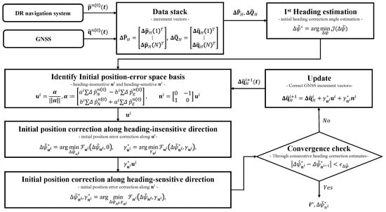
Figure 4. Flowchart of the proposed iterative process for the initial position correction.

To demonstrate the feasibility of real-time implementation, we evaluate the computational complexity of the proposed method. The MGPA method described in Section 2 has a time complexity of $O\left(N\right)$ due to its closed-form solution using N pairs of position increment vectors. Given the typically small sample size (e.g., $N=20$), this imposes a negligible computational load. Building on this, the complexity of the proposed IPC-MGPA is derived as $O(K·M·N)$. This formulation accounts for the K iterations required for convergence and M steps involved in the 1D search algorithm. The factor N accounts for the processing of all position samples required for both the identification of basis vectors and the initial heading estimation at each step. Although the computational load of the proposed method is higher than that of the conventional MGPA, the values of K and M are all small, and thus the absolute increase in computation remains limited. Consequently, the overall computation remains sufficiently lightweight for real-time implementation on the AUV.

4. Experiments

4.1. Experimental Setup

To validate the proposed initial position correction method, sea experiments were conducted using the AUV shown in Figure 5. The platform is equipped with a Fiberpro IMU (Fiberpro, Inc., Daejeon, Republic of Korea), a Teledyne Pathfinder DVL (Teledyne RD Instruments, Poway, CA, USA), a PNI Field Force TRAX digital compass (PNI Sensor, Windsor, CA, USA), and a single-antenna NovAtel OEM719 GNSS receiver (NovAtel Inc., Calgary, AB, Canada). The key specifications of each sensor are listed in Table 1. The sensor noise parameters listed in Table 1 are applied to an integrated navigation system (SINS, DVL) and used to calculate the iteration threshold $\left({ϵ}_{\mathrm{\Delta }\widehat{\psi }}\right)$ of the proposed method. However, unlike internal sensors (IMU, DVL, Digital Compass), GNSS performance is highly sensitive to external environmental factors such as sea state. In such conditions, relying on fixed datasheet values may cause the algorithm to overfit to transient GNSS noise, ultimately degrading the alignment performance. Therefore, while the nominal datasheet values were applied in this study, as they were deemed appropriate for the observed environment, adjusting the GNSS uncertainty parameter may be necessary in general practical applications to ensure robustness.

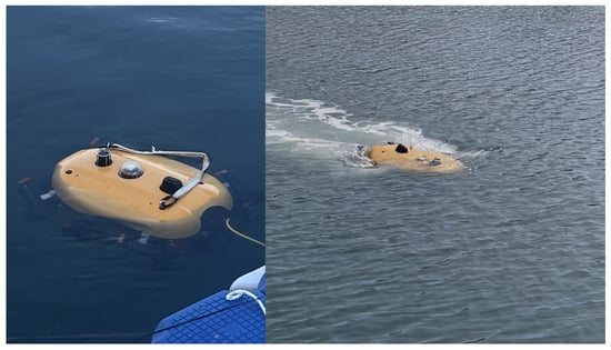
Figure 5. The AUV platform used for sea trials.

Table 1. Specifications of sensor equipped in the AUV.

Sensor	Parameter	Value
IMU	Gyroscope in-run bias stability	≤0.05°/h
	Gyroscope angle random walk	$0.025°/\sqrt{\mathrm{h}}$
	Accelerometer in-run bias stability	3 μg
	Accelerometer velocity random walk	0.015 $\mathrm{m}/\mathrm{s}\sqrt{\mathrm{h}}$
	Sampling rate	100 $\mathrm{Hz}$
DVL	Long term accuracy	$\pm 0.2\%\pm 0.1$ $\mathrm{cm}/\mathrm{s}$
	Precision	$\pm 0.5$ $\mathrm{cm}/\mathrm{s}$
	Resolution	$0.01$ $\mathrm{mm}/\mathrm{s}$
	Sampling rate	<12 $\mathrm{Hz}$
Digital compass	Heading accuracy	$0.3°$ $\mathrm{rms}$
	Heading resolution	$0.1°$
	Roll, pitch accuracy	$0.2°$ $\mathrm{rms}$
	Roll, pitch resolution	$0.01°$
	Sampling rate	<30 $\mathrm{Hz}$
GNSS	Horizontal position accuracy	$1.5$ $\mathrm{m}\mathrm{rms}$
	Sampling rate	1 $\mathrm{Hz}$

The AUV operated along two distinct trajectories. Their paths are shown in Figure 6 and Figure 7, and the travel distances and durations are summarized in Table 2. As shown in both figures, the AUV operated on the sea surface to ensure continuous GNSS signal reception. Although AUVs are typically operated underwater, the surface operation conducted in this experiment served two purposes: acquiring the GNSS positions need for heading correction of the alignment methods consider in this study, including MGPA and IPC-MGPA, and logging GNSS positions as reference data for evaluating alignment performance.

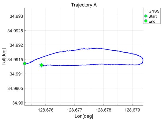
Figure 6. Experimental trajectory A represented by GNSS positions.

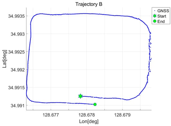
Figure 7. Experimental trajectory B represented by GNSS positions.

Table 2. Travel distance and duration of the experimental trajectories.

Trajectory	A	B
Travel distance [m]	843.39	1320.44
Travel duration [s]	786.94	1208.37

During the operation, the AUV’s position and attitude were estimated by DR using the integrated navigation system (SINS/DVL). The initial position and attitude for DR were obtained from GNSS and a digital compass, respectively. For initial heading alignment, GNSS positions were collected for approximately 20 s at 1 Hz. This period was determined based on the operational scenario to minimize surface residence time, and preliminary tests confirmed that it is the minimum sampling length required to ensure adequate heading estimation performance. Once 20 samples were collected, the initial heading alignment was performed using the DR positions corresponding to the GNSS epochs. Upon completion, the previous position and attitude were adjusted using the estimated initial heading and, in the case of the proposed method, the corrected initial position of IPC-MGPA. Thereafter, until the end of the operation, navigation proceeded by DR only, while GNSS measurements were logged for evaluation but not applied for navigation.

To evaluate the performance of the proposed method, we conducted a comparative experiment. We compared the navigation results using different alignment methods while keeping the DR configuration and algorithm identical: (I) MGPA, which estimates only the initial heading; (II) RHA, a trajectory matching-based method referred to as rapid heading alignment in this study [17]; and (III) IPC-MGPA, which corrects the initial position and estimates the initial heading based on the corrected position. This comparative experiment was conducted for both Trajectories A and B. Due to the absence of a high-performance reference system (e.g., RTK-GNSS, precision AHRS) on the platform, a direct heading measurement for evaluating the performance of the alignment methods was not available. Therefore, the performance was assessed indirectly using the Euclidean distance error between the navigation results produced by each alignment method and the GNSS positions. The mean of this distance error served as the primary metric.

4.2. Experimental Results

Figure 8 and Figure 9 show the experimental navigation results for trajectories A and B, respectively. In both figures, the red dot plot depicts the DR trajectory obtained using the MGPA alignment (hereafter, MGPA trajectory), and the cyan dot plot depicts the trajectory obtained using the RHA alignment (hereafter, RHA trajectory). The black dot plot depicts the trajectory obtained using the proposed IPC-MGPA alignment (hereafter, IPC-MGPA trajectory).

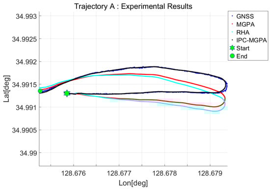
Figure 8. Experimental results in trajectory A. The DR trajectories aligned by MGAP, RHA, and IPC-MGPA are represented by red, cyan, and black dots, respectively.

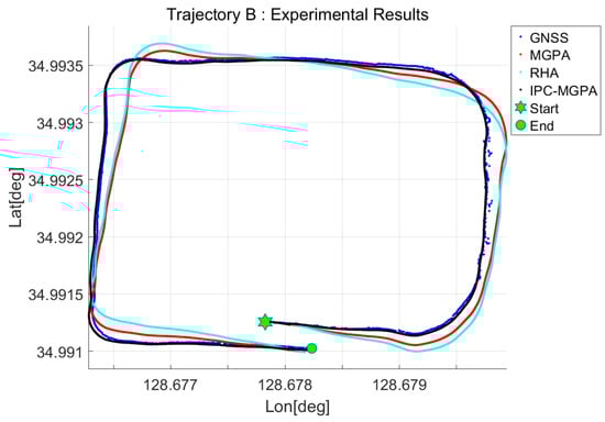
Figure 9. Experimental results in trajectory B. The DR trajectories aligned by MGAP, RHA, and IPC-MGPA are represented by red, cyan, and black dots, respectively.

As these experiments were conducted under identical DR conditions, varying only the initial heading alignment method, the resulting MGPA, RHA, and IPC-MGPA trajectories in Figure 8 and Figure 9 are visibly divergent. Visually, the IPC-MGPA trajectory aligns much more closely with the GNSS reference trajectory than the MGPA and RHA trajectory; This difference is also quantitatively represented by the calculated mean Euclidean distance errors presented in Table 3.

Table 3. Navigation results per alignment methods.

Mean Euclidean Distance Error [m]
Alignment Method	Trajectory A	Trajectory B
MGPA	16.866	15.827
RHA	21.750	27.970
IPC-MGPA	2.401	2.439

Figure 10 and Figure 11 present a comparison of the coordinates in the north–east plane of the local NED frame, adjusted by MGPA and IPC-MGPA during the 20-s initial alignment for trajectories A and B, respectively. These figures also plot the north–east plane coordinates obtained from the GNSS and DR positions, both referenced to the initial GNSS position. During the initial alignment phase, the estimated heading showed significant differences between the MGPA and IPC-MGPA method. For trajectory A, the estimated headings obtained from MGPA and IPC-MGPA were $91.{64}^{\circ }$ and $98.{58}^{\circ }$. In the case of trajectory B, they were $110.{83}^{\circ }$ and $106.{01}^{\circ }$, respectively. This discrepancy is attributed to the error present in the initial GNSS position. In both figures, the initial GNSS position is visibly offset from the overall path defined by the subsequent GNSS positions. This caused the MGPA method to be misaligned with the true path. In contrast, the IPC-MGPA method corrected this initial position offset, resulting in an aligned path that shares a similar orientation with the GNSS reference trajectory.

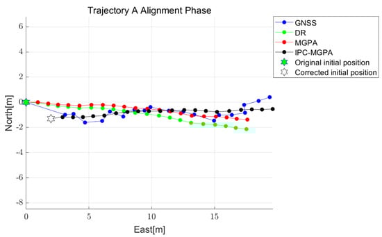
Figure 10. Variation of the north-east plane coordinates during the initial alignment for trajectory A. The plot shows the GNSS positions, DR positions, reference to the initial GNSS position, and the positions adjusted by MGPA and IPC-MGPA, respectively.

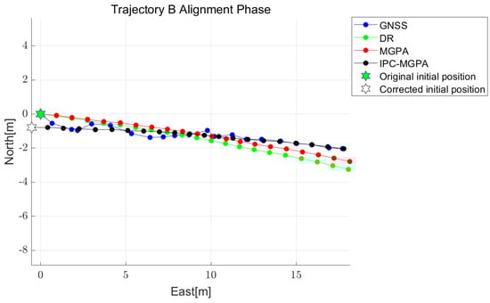
Figure 11. Variation of the north-east plane coordinates during the initial alignment for trajectory B. The plot shows the GNSS positions, DR positions, reference to the initial GNSS position, and the positions adjusted by MGPA and IPC-MGPA, respectively.

To verify that the performance of the proposed IPC-MGPA is statistically significant and not limited to the first alignment segment, an additional set of 100 time segments was defined for the initial alignment, and quantitative comparison experiments were conducted for each trajectory. Here, the i-th segment performs alignment using a 20 s window starting at i-seconds, excluding the first i-seconds of the logged sensor data. After performing the initial alignment for each segment, the subsequent trajectory was estimated by DR, as in prior experiments. Finally, for each alignment segment, the resulting DR trajectory was compared with the GNSS trajectory to compute the mean Euclidean distance error. In addition, to ensure a comprehensive evaluation, this segment-based analysis was expanded to include experiments across varying alignment lengths of 20 s, 30 s, and 40 s.

The results of this experiment are represented in Figure 12 and Figure 13. For trajectory A, the IPC-MGPA outperformed MGPA in 71, 70, and 65 segments for alignment length of 20 s, 30 s, and 40 s, respectively. Against RHA, it demonstrated superior performance in 74, 76, and 73 segments for the same lengths. This dominance was similarly observed in trajectory B, where IPC-MGPA surpassed MGPA in 84, 72, and 70 segments, and outperformed RHA in 84, 77, and 72 segments across the 20 s, 30 s, and 40 s cases. Furthermore, IPC-MGPA demonstrated superior performance not only in segment-wise comparison but also in the overall statistics, showing a lower mean and variance of the mean Euclidean distance errors. These comprehensive statistical results are summarized in Table 4. The 100 segments were additionally used to demonstrate the rapid convergence of the proposed iteration-based algorithm. Specifically, the number of iterations required for convergence ranged from 2 to 8 for trajectory A and from 2 to 9 for trajectory B.

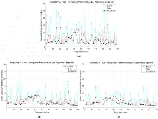
Figure 12. Navigation error comparison from the 100-segment experiment on Trajectory A with varying alignment sampling lengths. Each point represents the mean Euclidean error from an independent alignment segment. The plots correspond to alignment lengths of (a) 20 s, (b) 30 s, and (c) 40 s.

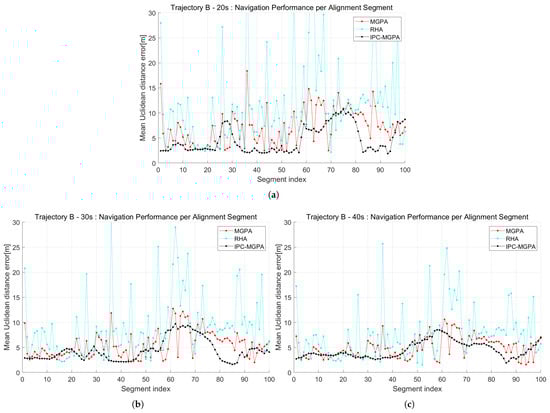
Figure 13. Navigation error comparison from the 100-segment experiment on Trajectory B with varying alignment sampling lengths. Each point represents the mean Euclidean error from an independent alignment segment. The plots correspond to alignment lengths of (a) 20 s, (b) 30 s, and (c) 40 s.

Table 4. Statistical comparison of navigation errors from the 100-segment experiment.

Alignment Length	Alignment Method	Trajectory A		Trajectory B
		Mean [m]	Variance [m2]	Mean [m]	Variance [m2]
20 s	MGPA	6.094	11.022	7.060	12.811
	RHA	9.031	40.658	11.562	68.027
	IPC-MGPA	3.857	4.071	4.591	7.207
30 s	MGPA	4.515	5.239	5.508	6.8914
	RHA	6.904	19.410	9.093	37.4118
	IPC-MGPA	3.483	3.592	4.389	4.8064
40 s	MGPA	3.797	3.204	4.952	4.454
	RHA	5.712	12.146	7.727	25.362
	IPC-MGPA	3.219	2.578	4.506	2.693

In summary, the experimental results demonstrate a consistent trend where the alignment performance of all three methods generally improves as the alignment length increases. Despite this common trend, the proposed IPC-MGPA consistently outperformed both MGPA and RHA across all tested cases. Notably, IPC-MGPA exhibited not only the lowest mean error but also the smallest variance in most cases, indicating a relatively high degree of stability in alignment accuracy. As analyzed in Figure 10 and Figure 11, this stability stems from the proposed method’s capability to actively correct the initial position error, which is the critical factor degrading MGPA performance in SPP-based environments. In contrast, the relatively inferior performance of RHA is due to its reliance on high-precision GNSS measurements, making it less effective when using the SPP-based GNSS data employed in this study.

5. Conclusions

In this paper, we proposed a method to correct the initial position and thereby improve the performance of in-motion initial heading alignment based on multiple GNSS positions (MGPA) for AUVs. When the initial position is obtained from standard point positioning (SPP) GNSS, it can contain a large error, which not only degrades the heading alignment itself but also introduces an offset into all subsequent dead-reckoning (DR) positions. To overcome this problem, the proposed method iteratively corrects the initial position within the alignment process. The core idea is to decompose the coupled 2D optimization problem by identifying an orthogonal basis in the initial position-error space. The initial position is corrected along these basis directions, and the heading is then estimated from the corrected position.

The effectiveness of the proposed method was validated through sea trials involving two trajectories. In both cases, the proposed IPC-MGPA correcting the initial position error led to improved alignment accuracy and reduced DR position error compared with both the MGPA and RHA methods. Furthermore, to confirm that the improvement was not specific to the initial positions of these two paths, we defined multiple alignment segments with lengths of 20, 30, and 40 s within each trajectory and conducted independent experiments. Across these segments, the proposed method showed better performance in most segments and achieved lower mean errors and variances overall. These results demonstrate that compensating for the uncertainty in the GNSS-derived initial position enables more stable estimation of the initial heading.

This study evaluated the performance of the proposed method indirectly through navigation errors, as a high-precision reference heading was not available for direct validation. Future work should therefore include verification of the proposed method in an environment where such reference data can be obtained. Furthermore, the alignment process in this study relied on several assumptions for computational simplicity. Future study will also be necessary to develop alignment methods that account for these additional uncertainty factors.

References

- Wang, D.; Xu, Y.; Zhang, T.; Zhu, Y. A novel SINS/DVL tightly integrated navigation method for complex environment. IEEE Trans. Instrum. Meas. 2020, 69, 5183–5196. [Google Scholar] [CrossRef]
- Cho, G.R.; Kang, H.; Kim, M.-G.; Lee, M.-J.; Li, J.-H.; Kim, H.; Lee, H.; Lee, G. An experimental study on trajectory tracking control of torpedo-like AUVs using coupled error dynamics. J. Mar. Sci. Eng. 2023, 11, 1334. [Google Scholar] [CrossRef]
- Tal, A.; Kelin, I.; Katz, R. Inertial navigation system/Doppler velocity log (INS/DVL) fusion with partial DVL measurements. Sensors 2017, 17, 415. [Google Scholar] [CrossRef] [PubMed]
- Titterton, D.H.; Weston, J.L. Strapdown Inertial Navigation Technology, 2nd ed.; Institution of Electrical Engineers: London, UK, 2004. [Google Scholar]
- Ma, C.; Zhou, S.; Wang, Z.; Zhang, H.; Xu, L.; Miao, J. In-motion fine alignment algorithm for AUV based on improved extended state observer and Kalman filter. Meas. Sci. Technol. 2024, 35, 126305. [Google Scholar] [CrossRef]
- Tsukerman, A.; Kelin, I. Analytic evaluation of fine alignment for velocity aided INS. IEEE Trans. Aerosp. Electron. Syst. 2017, 54, 376–384. [Google Scholar] [CrossRef]
- Dong, Q.; Li, Y.; Sum, Q.; Zhang, Y. An adaptive initial alignment algorithm based on variance component estimation for a strapdown inertial navigation system of AUV. Symmetry 2017, 9, 129. [Google Scholar] [CrossRef]
- Wu, M.; Wu, Y.; Hu, X.; Hu, D. Optimization-based alignment for inertial navigation systems: Theory and algorithm. Aerosp. Sci. Technol. 2011, 15, 1–17. [Google Scholar] [CrossRef]
- Li, W.; Tang, K.; Lu, L.; Wu, Y. Optimization-based INS in-motion alignment approach for underwater vehicles. Optik 2013, 124, 4581–4585. [Google Scholar] [CrossRef]
- Zhu, B.; Li, J.; Cui, G. Robust optimization-based alignment method based on projection statistics algorithm. IEEE Sens. J. 2021, 21, 16538–16546. [Google Scholar] [CrossRef]
- Chang, L.; Li, J.; Li, K. Optimization-based alignment for strapdown inertial navigation system: Comparison and extension. IEEE Trans. Aerosp. Electron. Syst. 2016, 52, 1697–1713. [Google Scholar] [CrossRef]
- Raskaliyev, A.; Patel, S.H.; Sobh, T.M.; Ibrayev, A. GNSS-based attitude determination techniques-a comprehensive literature survey. IEEE Access 2020, 8, 24873–24876. [Google Scholar] [CrossRef]
- Bing, W.; Lifen, S.; Guorui, X.; Yu, D.; Guobin, Q. Comparison of attitude determination approaches using multiple Global Positioning System (GPS) antennas. Geod. Geodyn. 2013, 4, 16–22. [Google Scholar] [CrossRef]
- Chang, G.; Xu, T.; Wang, Q.; Li, S.; Deng, K. GNSS attitude determination method through vectorisation approach. IET Radar Sonar Navig. 2017, 11, 1477–1482. [Google Scholar] [CrossRef]
- Sun, R.; Cheng, Q.; Wang, J. Precise vehicle dynamic heading and pitch angle estimation using time-difference measurements from a single GNSS antenna. GPS Solut. 2020, 24, 84. [Google Scholar] [CrossRef]
- Groves, P.D.; Handly, R.J.; Parker, S.T. Vehicle heading determination using only single-antenna GPS and single gyro. In Proceedings of the 22nd International Technical Meeting of the Satellite Division of The Institute of Navigation, Savannah, Georgia, 22–25 September 2009. [Google Scholar]
- Chen, Q.; Lin, H.; Kuang, J.; Luo, Y.; Niu, X. Rapid initial heading alignment for MEMS land vehicular GNSS/INS navigation system. IEEE Sens. J. 2023, 23, 7656–7666. [Google Scholar] [CrossRef]
- Wu, Q.; Chai, H.; Xiang, M.; Zhang, Y.; Feng, X. Rapid in-motion heading alignment using time-difference carrier phases from a single GNSS antenna and a low-grade IMU. Meas. Sci. Technol. 2024, 35, 106302–106319. [Google Scholar] [CrossRef]
- Choo, J.; Lee, G.; Lee, P.-Y.; Kim, H.S. Position based in-motion alignment method for an AUV. J. Inst. Control. Robot. Syst. 2020, 26, 649–659. [Google Scholar] [CrossRef]
- Lee, G.; Choi, K.; Lee, P.-Y.; Kim, H.S.; Kang, H.; Lee, J. Performance enhancement technique for position-based alignment algorithm in AUV’s navigation. J. Inst. Control. Robot. Syst. 2023, 29, 740–747. [Google Scholar] [CrossRef]
- Choi, K.; Lee, G.; Lee, P.-Y.; Kim, H.S.; Kang, H.; Lee, J. Heading bias estimation algorithm for autonomous underwater vehicles considering angular accuracy. J. Inst. Control. Robot. Syst. 2025, 31, 124–130. [Google Scholar] [CrossRef]
- Liu, W.; Cheng, X.; Ding, P.; Cao, P. An optimal indirect in-motion coarse alignment method for GNSS-aided SINS. IEEE Sens. J. 2022, 22, 7608–7618. [Google Scholar] [CrossRef]
Disclaimer/Publisher’s Note: The statements, opinions and data contained in all publications are solely those of the individual author(s) and contributor(s) and not of MDPI and/or the editor(s). MDPI and/or the editor(s) disclaim responsibility for any injury to people or property resulting from any ideas, methods, instructions or products referred to in the content. |
© 2025 by the authors. Licensee MDPI, Basel, Switzerland. This article is an open access article distributed under the terms and conditions of the Creative Commons Attribution (CC BY) license (https://creativecommons.org/licenses/by/4.0/).