Implementing Deep Learning Techniques in Port Agitation Studies Under the Context of Climate Change

Abstract

Climate change is impacting atmospheric patterns and therefore wave conditions, with ports being among the most affected infrastructures, making it crucial to ensure their operability under changing climatic conditions. Most scientific studies on climate change focus on coastal erosion and flooding, whereas research on its impact on port operability remains relatively scarce. This challenge could be tackled with the emergence of Artificial Intelligence (AI), where alternative modeling approaches can be developed. Thus, a novel AI-based model specifically designed for studying port agitation is introduced herein. By integrating a hybrid deep learning approach, combining Feedforward Neural Networks (FFNNs) to model wave climate and Convolutional Neural Networks (CNNs) for port image analysis, port agitation has been successfully predicted compared to linear wave propagation models. This marks the first instance of utilizing image processing tools to analyze port agitation, resulting in a model with a remarkably low error rate, while offering a significant reduction in computational time compared to traditional wave propagation models, reducing computational time by a factor of four to ten. The accuracy of the proposed model has been investigated and validated for the Port of Valencia, located in the Spanish section of the Mediterranean Sea.

1. Introduction

In 1992, the United Nations Framework Convention on Climate Change recognized climate change for the first time as a global issue. One of the ecosystems most threatened by climate change is coastal ecosystems. Approximately 40% of the world’s population lives within 100 km of a coastline and it is expected to rise to 75% by 2050 [1,2]. If necessary adaptation measures are not taken, it is projected that between 0.2% and 4.6% of the world’s population will experience annual flooding by the year 2100, with corresponding losses of 0.3% to 9.3% of the global Gross Domestic Product (GDP) [3]. Between 1984 and 2015, there was a net loss of 14,000 ${\mathrm{km}}^2$ of land due to erosion, while 24% of beaches eroded at rates exceeding 0.5 m/year [4,5]. Referring to ports, between 80% and 90% of the world’s goods are transported by sea and it is expected to increase by 4% within five years [6,7,8]. This means that a significant portion of the global economy depends on the proper functioning of navigation routes and ports. However, unlike coastal systems, there are not as many studies analyzing the potential impacts of climate change on ports. This disparity may be attributed to the scarcity of regional and local data necessary for conducting climate change assessments on ports [9]. In comparison to the scientific effort dedicated to the study coastal systems and beaches, the number of studies involving port areas is much lower [10] and the need for conducting climate studies becomes even more significant for ports located in vulnerable areas.

The impact of climate change will not be uniform across all countries. Certain regions will be more severely affected, with the Mediterranean basin standing out as one of the most threatened areas. It has been calculated that temperatures in the Mediterranean will increase by 1.4 °C with respect to pre-industrial levels, which is 20% more than in the rest of the world [11]. Given these forecasts, it becomes imperative to channel our efforts into studying the repercussions of climate change on critical hubs such as ports in highly vulnerable regions like the Mediterranean Sea. One of the first studies on ports and wave climate was conducted by Casas-Prat and Sierra [12,13] in which they studied how changes in wave direction would affect port agitation in the Catalan coast, while the effect of climate change on Catalan ports was investigated by Sierra et al. [14]. However, the great majority of the studies tackle the climate change assessment on ports from an administrative, institutional and planning perspective [15,16,17,18], while most of the studies concerning ports and climate change address this problem from a global point of view [19,20,21,22,23,24,25,26,27,28,29,30,31,32,33,34].

Referring to local and regional studies, Sánchez-Arcilla et al. [35] conducted a review on the potential impacts of climate change in the Mediterranean Sea, while Sierra et al. [36] studied how green measures could mitigate these impacts. Diaz-Hernandez et al. [37] analyzed the influence of infragravity waves on ports and applied it to a specific case in the Port of Geraldton. Laxe et al. [38] evaluated the sustainability of Spanish ports, while Velasco et al. [39] compared the effectiveness of structural and non-structural measures to cope with climate change in the city of Barcelona. Vinet et al. [40] mapped flood-related mortality in the Mediterranean Basin and Gracia et al. [41] assessed the impact of SLR on port operability in the Catalan Coast. However, the number of studies that assess the operability of specific ports under different climate change scenarios significantly decreases, Sierra et al. [42] studied the port of Barcelona, Camus et al. [43] analyzed port operation in the North of Spain, Jebbad et al. [44] evaluated the operability of the port of Tangier-Med and Sierra et al. [45] assessed the Balearic ports.

Most scientific studies assessing port operability or studying agitation within ports rely heavily on numerical wave propagation models. These phase-resolving or phase-averaged models, in order to consider wave diffraction and wave non-linearities, require a high computational cost. Only Kankal and Yüksek [46] and López and Iglesias [47] used an alternative approach implementing Artificial Neural Networks (ANNs), but they primarily focused on climate propagation from deep water to buoys, more aligned with wave downscaling than the examination of port operability [48]. Over the past few years, the evolution of Artificial Intelligence (AI) has been remarkable, emerging as a promising tool that reshapes traditional methodologies in many different fields. Ocean and maritime engineering is one of those fields in which AI has advanced rapidly in recent years. However, within seaports, a notable lack of AI-driven wave forecasting models is observed, highlighting a significant research gap in this area [49]. Nevertheless, Chondros et al. [50] enhanced a mild-slope wave model using neural networks for port applications, while Zheng et al. [51,52] coupled a non-linear Boussinesq and spectral, respectively, wave model with an ANN model for wave forecasting in ports. Primarily, AI technologies have been applied in the prediction and characterization of offshore wave conditions [53,54,55], yielding highly encouraging results. Yet, the presence of AI technologies in port agitation studies is almost negligible. Thus, there is a strong rationale for implementing this technology, since one of its key advantages is the substantially lower computational cost, whereas tradition port agitation models are typically characterized by high complexity and significant computational demands.

The present study addresses the issue of port agitation with an AI approach aligning with the works of Kankal and Yüksek [46] and López and Iglesias [56] trying to promote and advance in the application of AI techniques to traditional wave propagation models, which often entail high computational costs. A pioneering hybrid deep learning model based on Convolutional Neural Networks (CNNs) and Feed Forward Neural Networks (FFNNs) is introduced, based on wave climate characteristics and images to study port agitation. FFNNs incorporate wave climate data into the model and CNNs tackle the images of the port, with the final aim of having a detailed and complete characterization of the problem and exploiting all the data in an optimal framework. To the authors knowledge, it is the first instance of an Artificial Intelligence (AI) based model for studying port operability within the framework of climate change. A detailed explanation is provided regarding the development of deep learning models so that it can serve as a guide for future studies. Few articles, even within the entire field of ocean engineering, thoroughly explain how these types of models should be constructed. This lack of detailed explanation hinders their implementation despite the significant advantages they offer. Moreover, it stands as the first model in the field of ocean and coastal engineering to utilize a deep learning approach that combines both data and images. This approach enables a substantial reduction in computational time and resource demands while maintaining high levels of accuracy.

The proposed model is implemented and validated in the Port of Valencia, Spain, enabling the evaluation of wave agitation under diverse climate change scenarios. The Port of Valencia was herein selected as a case study due to its strategic relevance, high exposure to climate-induced impacts and active involvement in AI-driven innovation initiatives (ECCLIPSE project). Located within a coastal zone identified as highly susceptible to SLR, the port is projected to experience an increased frequency and intensity of storm events. Furthermore, its distinct geomorphological characteristics and spatial orientation render it as a climate-sensitive infrastructure system, which remains relatively underexplored in this context [57].

The research methodology of the present study is illustrated in Figure 1. Initially, historical data are utilized to conduct a statistical extreme wave analysis, while through MonteCarlo simulations, a synthetic dataset is generated including future climate change conditions (Section 2.1). Both datasets are subsequently introduced into the SWAN wave propagation model (Section 2.1) to accurately simulate the transformation of offshore wave conditions toward the nearshore zone for port agitation assessment. The resulting outputs are then provided as boundary conditions for the MILDwave model (Section 2.2), as well as for the proposed AI model. The AI model is developed in Section 3 with a hybrid FFNN–CNN architecture, while FFNNs and CNNs are described in Section 2.3. The numerical predictions obtained from MILDwave are used to train and validate the hybrid AI model (Section 4), facilitating an AI port agitation study for diverse wave conditions in the Port of Valencia (Section 4).

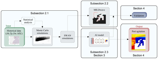
Figure 1. Workflow of the research framework utilized in the present study. The framework encompasses statistical analysis of historical data, Monte Carlo simulations, SWAN modeling, MILDwave modeling, development and validation of the AI model and the resulting wave agitation assessment.

2. Methodology

The methodology outlined in this section unfolds in three primary stages: (a) the gathering and propagation of wave climate data to the coastline (Section 2.1), (b) the formulation of the port agitation model (Section 2.2) and (c) the principles of an AI-driven surrogate model (Section 2.3).

2.1. Data Collection and Wave Climate Propagation

The first step to develop a port agitation model is to collect the data on wave climate and study the area of interest. In this case, the area of study is the area of Valencia, Spain, which is located in the Western Mediterranean section (Figure 2). To conduct the study, the deep water Valencia buoy was used and historical hourly significant wave height ($Hs$), peak wave period ($Tp$) and wave direction ($Dir$) records were downloaded from [58], which is the official website of the Spanish Authority in charge of characterizing wave climate. Moreover, wind parameters obtained from the same source were also taken into consideration as secondary parameters for the wave propagation model.

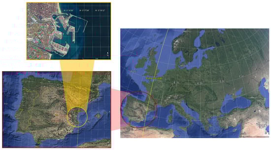
Figure 2. Satellite images from Google Earth illustrating a zoom sequence from the European continent to the country of Spain and to the Port of Valencia.

All the historical data were carefully preprocessed, which is a crucial step in developing AI models. To ensure efficiency, the dataset must be homogeneous, balanced and free of temporal gaps. After preprocessing the historical series, a thorough statistical analysis was performed. This included studying time records in Valencia from 2005 to 2025, focusing on trends and statistical parameters. Once this analysis was complete, Level III probabilistic methodologies, specifically Monte Carlo simulations, were applied to generate a synthetic database covering the period from 2025 to 2050. This synthetic dataset was then merged with the historical records (2005–2025) to create a complete database, which served as the foundation for developing the AI model. All details about the research area, climate data, preprocessing tasks, future climate projections, Monte Carlo simulations and generation of synthetic data series are described within [59], as the present study is an extension of that work.

To propagate these wave climate conditions from deep water to shallow water, encompassing both present and future climate scenarios, the numerical model SWAN [60] was used. For this purpose, a Digital Terrain Model (DTM) was developed based on the bathymetry data from [61] and the WGS84/UTM Zone 30N Geodesic System. The current study utilized two model grids: an outer and a nested grid. The use of multiple grids aims to enhance resolution and accuracy. The outer grid features square elements with a resolution of 200 m and dimensions of 46,400 m × 39,800 m, consisting of 232 x-nodes and 199 y-nodes.

The SWAN model version employed was 41.31AB, operating with an implicit integration scheme. During simulations, the model was configured to run in stationary mode with the third-generation option (GEN3) activated. The model physics included whitecapping parameterization with a coefficient for determining the rate of whitecapping dissipation $C_{ds}=2.36·{10}^{-5}$[62], depth limited wave breaking with breaker parameter equal to $0.73$ and dissipation scaling factor equal to 1 [63], bottom friction with bottom friction coefficient $C_b=0.038$${\mathrm{m}}^2·$${\mathrm{s}}^{-3}$[64], quadruplet interactions with frequency separation parameter $\lambda =0.25$ and empirical scaling coefficient $C_{nl4}=3·{10}^7$ using the Discrete Interaction Approximation (DIA) and refraction at its default settings [62].

The model spectrum considered 36 frequencies (ranging from 0.0356 Hz to 1.00 Hz) and 72 directions. The shape of the spectra was determined by the JONSWAP spectrum (with two sets of peak enhancement factors $\gamma$ and spectral width parameters $\sigma$: $\gamma =10$, $\sigma =10$/$\gamma =3.3$, $\sigma =20$), depending on the energy of the incident waves, which varied according to wave height. The forcing functions of the wave data were uniformly applied across the entire model domain, with sea level set at +0.00 m (above LAT), while currents were neglected.

2.2. Port Agitation Numerical Model

After propagating the wave climate to coastal waters, the next step involved the development of a numerical model tailored to analyze wave agitation within the Port of Valencia. Phase-resolving numerical models, mainly classified in three subtypes Boussinesq equation models, mild-slope equation models and non-hydrostatic equation models, are commonly used in port agitation studies. In this study, the MILDwave model developed by Troch [65] was selected to study wave agitation, based on the mild-slope equations of Radder and Dingemans [66] (Equations (1) and (2)):

$$\begin{array}{cc}\hfill {\displaystyle \frac{\partial \eta }{\partial t}}& =B\varphi -\nabla (A\nabla \varphi )\hfill \end{array}$$

(1)

$$\begin{array}{cc}\hfill {\displaystyle \frac{\partial \varphi }{\partial t}}& =-g\eta \hfill \end{array}$$

(2)

$$\begin{array}{cc}\hfill A& ={\displaystyle \frac{C{C}_g}{g}}\hfill \end{array}$$

(3)

$$\begin{array}{cc}\hfill B& ={\displaystyle \frac{{\omega }^2-k^{2}C{C}_g}{g}}\hfill \end{array}$$

(4)

where t is the time, $\eta$ the surface elevation at the still water level, $\varphi$ the velocity potential at the still water level, A and B coefficients calculated by Equations (3) and (4), g the gravitational acceleration, C is the phase velocity, $C_g$ the group velocity, $\omega$ the angular frequency and k the wave number.

MILDwave employs a finite difference scheme to solve these equations, applying central differences for both spatial and temporal derivatives. The computational domain is discretized into grid cells with dimensions $\Delta x$ and $\Delta y$, along X-axis and Y-axis, where $\varphi$ (Equation (5)) and $\eta$ (Equation (6)) are solved at every $(n+1)\Delta t$ and $(n+1/2)\Delta t$ time levels, respectively, at the center of each grid cell:

$${\varphi }_{i,j}^{(n+1)}\approxeq {\varphi }_{i,j}^n-g{\eta }_{i,j}^{(n+1/2)}\Delta t$$

(5)

$$\begin{array}{cc}\hfill {\eta }_{i,j}^{(n+1/2)}& \approxeq {\eta }_{i,j}^{(n-1/2)}+B_{i,j}{\varphi }_{i,j}^n\Delta t\hfill \\ \hfill & -{\displaystyle \frac{A_{i+1,j}-A_{i-1,j}}{2\Delta x}}{\displaystyle \frac{{\varphi }_{i+1,j}^n-{\varphi }_{i-1,j}^n}{2\Delta x}}\Delta t\hfill \\ \hfill & -A_{i,j}{\displaystyle \frac{{\varphi }_{i-1,j}^n-2{\varphi }_{i,j}^n+{\varphi }_{i+1,j}^n}{\Delta x^2}}\Delta t\hfill \\ \hfill & -{\displaystyle \frac{A_{i,j+1}-A_{i,j-1}}{2\Delta y}}{\displaystyle \frac{{\varphi }_{i,j+1}^n-{\varphi }_{i,j-1}^n}{2\Delta y}}\Delta t\hfill \\ \hfill & -A_{i,j}{\displaystyle \frac{{\varphi }_{i,j-1}^n-2{\varphi }_{i,j}^n+{\varphi }_{i,j+1}^n}{\Delta y^2}}\Delta t\hfill \end{array}$$

(6)

where $\Delta t$ represents the numerical model time step, superscript n denotes the relevant time step and superscripts i and j the relevant cell of the grid.

MILDwave is capable of generating both regular and irregular waves, including long and short crested waves, at any chosen wave direction, utilizing a single wave generation line to ensure a homogeneous wave field. Numerical absorption sponge layers are implemented near the outer boundaries parallel to the wave generation line, where at each time step an absorption function is applied to the computed surface elevations, relaxing them across the span of the sponge layer. Furthermore, periodic lateral boundaries are implemented to ensure homogeneity of the wave field, particularly for oblique waves. This mechanism facilitates the transfer of numerical information from one side of the domain to the opposite side, enabling waves to propagate seamlessly across the computational domain. Boundaries are depicted with a distinct cell color which is assigned an absorption coefficient, herein used to control their reflection behavior. MILDwave considers almost all different transformation phenomena, namely absorption, refraction, shoaling, reflection, transmission, diffraction and wave breaking. Therefore, it represents a perfect model for simulating the agitation of the Port of Valencia without incurring extremely high computational costs or encountering significant numerical complexities that other numerical models might entail.

In this study, different wave cases were examined based on previously gathered data. MILDwave operates by introducing a unitary wave ($Hs=1$ m) to determine the disturbance coefficients $k_d=H_L/H_G$ within the port, where $H_L$ is the local significant wave height and $H_G$ the significant wave height at the wave generation boundary. Accordingly, testing focused on varying wave periods and wave directions, where from the full set of wave sea states, the most representative conditions were selected. In total, 6 different wave periods and 8 different wave directions, derived from the collected data, were tested, giving a total of 48 different wave condition cases. These cases are denoted as “$C_{Tp}$”. “$C_{Dir}$” cases, where $C_{Tp}$ corresponds to the wave period and $C_{Dir}$ to the wave direction, as outlined in Table 1. For example, case 3.6 would be the wave case with a wave period of 6.1 s (3.) and a direction of ${135}^{°}$(.6). The $Tp$ cases were selected based on the data collected from [58] and on the projections made for future time scenarios. For the wave direction, the same approach was follows, studying the swell rose (Figure 3) and dividing the main directions in sectors of $22.5^{°}$.

Table 1. Wave condition cases used for the port agitation study.

Case	Peak Wave Period $\mathit{Tp}$ (“${\mathit{C}}_{\mathit{Tp}}$”)	Wave Direction $\mathit{Dir}$ (“${\mathit{C}}_{\mathit{Dir}}$”)
1	8.9 s	$22.5^{°}$
2	7.4 s	$45.0^{°}$
3	6.1 s	$67.5^{°}$
4	5.6 s	$90.0^{°}$
5	5.0 s	$112.5^{°}$
6	4.6 s	$135.0^{°}$
7	-	$157.5^{°}$
8	-	$180.0^{°}$

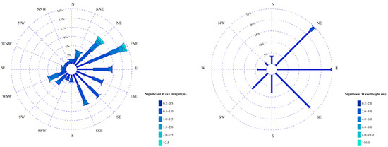
Figure 3. Swell rose outside the Port of Valencia, Spain, for long-term (left) and extreme (right) distribution [58].

Regarding the model settings, irregular waves were generated with the objective of producing approximately 1000 individual waves per case, while only the fully developed wave field was considered in the analysis. Sponge layers of 10 wavelengths were applied and 4 different absorption coefficients were used to model the different structures and objects within the Port of Valencia. The different absorption coefficients were tuned and validated before running the model to obtain the target reflection coefficients (Figure 4 and Table 2), which were 0.3 for armor layer units of the breakwaters (represented by colors cyan and green) and 0.9 for vertical walls (represented by color red). Once the wave condition cases were defined, the port layout geometry was sketched and the absorption coefficients were calibrated, all simulations were executed.

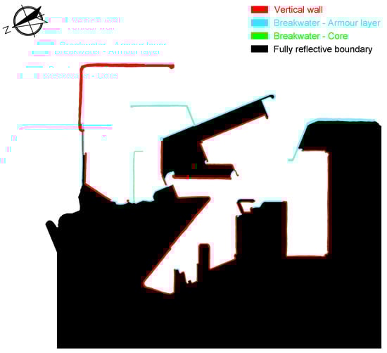
Figure 4. Top view of the Port of Valencia, Spain, as simulated in MILDwave. Red color indicates vertical walls, cyan and green colors represent breakwaters and black color denotes fully reflective boundaries. The view is oriented at 202.5° relative to North.

Table 2. MILDwave absorption coefficients assigned to each distinct cell color for boundaries.

Case	Cyan	Green	Red	White	Black
1	0.97	0.70	0.45	1.00	0.00
2	0.97	0.70	0.25	1.00	0.00
3	0.96	0.68	0.20	1.00	0.00
4	0.95	0.70	0.15	1.00	0.00
5	0.88	0.20	0.12	1.00	0.00
6	0.88	0.20	0.11	1.00	0.00

2.3. FFNNs and CNNs

After completing all numerical simulations, the dataset required to develop the AI-based surrogate model was fully prepared. For the AI model definition, Artificial Neural Networks (ANNs) are employed, with input parameters representing the wave conditions and port layout, while the output corresponds to the resulting wave agitation within the port. Between the different supervised learning techniques, ANNs are usually the most powerful, being able to extract complex relationships and especially recommended when dealing with images, as within the present study.

Integrating port layout information into the model was most effectively achieved through images, which were then combined with wave climate data. To incorporate the wave climate information, an FFNN was employed, whereas CNNs were utilized to process the port images. FFNNs are a widely adopted choice in ocean and coastal engineering due to its simplicity and efficacy in characterizing wave climate [67] and are therefore selected also for the present study. However, FFNNs may struggle with more complex processes, particularly in image processing tasks, where CNNs excel. In this scenario, CNNs emerged as the preferred option for their superior performance and adaptability. Compared to graph convolutional networks, which handle images with diverse topographical structures and varying sizes [68], CNNs are preferred herein due to the simplicity of the problem, where the port layout is represented as a 2D image with a standardized size and a regular pixel grid.

FFNN are ANNs that pass the information from one layer to another through transfer functions, mimicking the structure of the human brain. Each layer consists of various neurons and the complexity of processes the ANN can model increases with the number of neurons and layers. However, as the complexity grows, so does the computational cost and the risk of overfitting [48]. In the present approach, rather than employing the conventional shallow FFNNs commonly used in ocean engineering, a deeper FFNN composed of two hidden layers is chosen. These layers were then concatenated with the CNN that process the images of the ports. This allows to harness the benefits of both deep FFNNs and CNNs, creating a hybrid model capable of capturing the intricacies of the data while mitigating the risk of overfitting.

CNNs, unlike conventional ANNs, offer a distinct architecture tailored for tasks like image processing, while FFNNs rely on fully connected layers where neurons are interconnected between adjacent layers, CNNs employ a sequence of specialized layers, convolutional and pooling layers, designed for feature extraction and dimensional reduction [69]. In contrast to FFNNs, where the output is determined by connections between individual neurons, convolutional layers in CNNs are defined by three dimensions: (a) width, (b) height and (c) depth. Width and height correspond to the dimensions of the input images, while depth denotes the number of filters applied to extract the features of these images. Deeper layers can capture more intricate features, but this depth comes with increased computational demands. To manage this, pooling layers are often employed after convolutional layers to reduce computational overhead.

In the convolutional layer each filter is convolved across the width and height of the input volume following Equation (7) [70].

$$y_k^{\left(m\right)}=f_j\left(\sum _{c=1}^C{W}_k^{(c,m)}{x}_{k-1}^{\left(c\right)}+b_k^{\left(c\right)}\right)$$

(7)

where $y_k^{\left(m\right)}$ is the output of the convolutional layer k, $x_{k-1}^{\left(c\right)}$ the input from layer $k-1$, $W_k^{(c,m)}$ the $m^{\mathrm{th}}$ filter of channel c and $b_k^{\left(c\right)}$ the bias term.

In the convolutional layer, the weighted summation of the pixels is performed following the convolutional filter (kernel), producing a new output (Figure 5) [71]. Once the convolutional filter is applied to the image, the output of the convolutional layer is passed to the pooling layer. On the other hand, the pooling layer downsamples the output produced by the convolutional layers to avoid prohibitive models in terms of computational costs. Pooling layers divide the output of the convolutional layer into non overlapping regions that depends on the filter size and take commonly the average value (average pooling layers) or the maximum value (max pooling layers). In this case, max pooling layers were used (Figure 6).

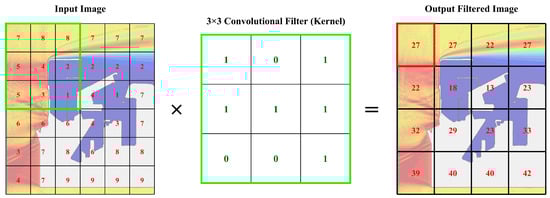
Figure 5. Schematic representation of the convolutional operation. A 3 × 3 convolutional filter (kernel) is applied to the input image, performing weighted summations over local pixel regions to generate an output filtered image.

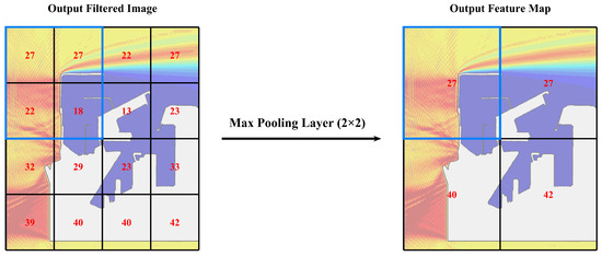
Figure 6. Schematic representation of the max-pooling operation. After convolution, the output filtered image is downsampled by dividing it into non-overlapping regions based on a 2 × 2 max pooling layer, with the maximum value from each region retained (max pooling), generating an output feature map.

To highlight the need to use specific types of neural networks when dealing with images due to the significant computational cost they entail, it is important to note that computers treat images as pixels and within each pixel there are three color channels (green, red and blue). Thus, each pixel implies three digital components, a number from 0 to 255 representing the red, green and blue colors (RGB code), whose combination gives the pixel value. Consequently, an image of 1000 × 1000 pixels is associated with 3 million numbers. In our case, our images were 1728 × 1152 pixels, resulting in 1728 × 1152 × 3 numbers, totalling 5,971,968 numbers. Therefore, the need to use a specific methodology and a specific type of neural networks to deal with images.

3. Development of an AI Model for Port Agitation

The main objective of this research is to develop a pioneering AI model that can serve as an alternative and complimentary tool for numerical models of port agitation, which entail a high computational cost. To achieve this, the first step was to choose the most suitable type of AI to model the problem. As outlined in Section 2, a hybrid model of neural networks combining FFNNs and CNNs was chosen. For the development of the model, the libraries TensorFlow [72] and Keras DL were used [73] in Python 3.12 environment [60] in a CORE i7 8th Gen Intel (R) UHD Graphics 620 CPU with a 16 GB RAM memory. The Rectified Linear Unit (ReLU) activation function is used in the FFNN, while the Adam optimization algorithm is adopted to perform the training process.

The initial step in developing a data-driven model (ANNs) is data preprocessing. For CNNs to function properly, all input (port situation and geometric arrangement) and output images (port agitation) must share identical dimensions. Accordingly, all images were standardized to 1728 × 1152 pixels. Following this, all the images were normalized dividing each pixel value by 255, thereby scaling them to a range between 0 and 1. This procedure improves numerical stability and reduces computational cost during model training. The wave climate data, comprised significant wave heights, peak periods and wave directions, are normalized using a robust scaler, which centers the data around the median and scales it according to the interquartile range. This technique effectively mitigates the influence of outliers while preserving the physical relationships among variables, ultimately enhancing model performance and convergence.

With all datasets preprocessed, the model definition was carried out. A trial-and-error approach, commonly employed in ANN design, was adopted, beginning with an initial model configuration and subsequently optimizing its hyperparameters. The performance of the model was evaluated using the Mean Square Error (MSE) as the loss function (Equation (8)).

$$\mathrm{MSE}={\displaystyle \frac{1}{n}}\sum _{i=1}^n{(o_i-u_i)}^2$$

(8)

where $o_i$ represents the output of the model and $u_i$ denotes the real value. This loss function was selected over other commonly used metrics in image evaluation, such as the Structural Similarity Index (SSIM), due to its simplicity and its stronger emphasis on individual pixel accuracy. This choice aligns closely with the primary objective of our study, which is to identify areas within a port that are susceptible to agitation, prioritizing detailed pixel-level analysis.

The optimization process was initiated by defining the number of epochs and the batch size. The number of epochs serves as a hyperparameter, dictating how many times the neural network passes through the training dataset to discern patterns. Conversely, the batch size represents the quantity of data samples utilized by the ANN during each iteration of the epoch. In this study, epoch values ranging from 10 to 500 (Figure 7a) and batch sizes varying from 1 to 32 (Figure 7b) encompassing the entire training dataset were tested.

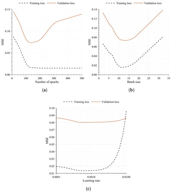
Figure 7. Optimization of the ANN hyperparameters: (a) number of epochs, (b) batch size and (c) learning rate. The training and validation losses are shown for each case, highlighting the balance between model accuracy and overfitting.

As observed, the training error steadily decreases with the number of epochs, yet beyond approximately 150 epochs, the reduction in error becomes marginal. Concurrently, the validation error begins to rise from around 100 epochs onwards, signaling overfitting. Consequently, the number of epochs was capped at 100 to mitigate overfitting. Regarding batch size, both, the training and validation errors reach their minimum at 12. Hence, the batch size was fixed at 12.

After defining the number of epochs and batch size, the learning rate was optimized. The learning rate determines the size of each step in the ANN training. Large learning rates adjust the ANN more aggressively and, consequently, are more computational efficient but can lead to instabilities or divergence of the model. In this case, learning rates from 0.0001 to 0.01 were tested, finding the optimal behavior at a learning rate of 0.0005 (Figure 7c).

Following this, the model architecture was optimized. The model of the study comprises two distinct branches: (a) an FFNN to incorporate wave climate data into the neural network and (b) a CNN to handle images. For the FFNN optimization, two hidden layers were selected. Although a single hidden layer is standard in coastal and ocean studies, enhancing the model’s complexity to effectively capture port agitation is pursued, aligning it with the capabilities of CNNs. With the chosen number of hidden layers, various architectures were explored, ranging from 4 to 8 neurons to 32–64 neurons. This approach was follows: to maintain coherence with CNNs, as CNN depths typically follow a power-of-2 pattern that increases with layer depth (Figure 8). As depicted in Figure 8, the training error remains relatively consistent across all FFNN architectures, while the validation error slightly rises with an increase in the number of neurons, suggesting potential overfitting. Furthermore, computational time escalates exponentially from the 8–16 architecture onwards. Consequently, the simplest architecture for the FFNN was chosen, 4–8.

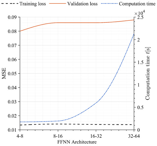
Figure 8. Optimization of the FFNN architecture, showing the evolution of training and validation loss together with computational time for different neuron configurations.

For the CNN architecture optimization, the same approach as with the FFNN was follows, testing different CNN architectures. Basing on previous works, the number of layers was set to three convolutional layers and two pooling layers [74]. Then, the architecture of each layer was optimized. As illustrated in Figure 9, significant increases in computational time is evident beyond the 8–16–32 architecture, going from 5951 s for the 8–16–32 architecture to 86,400 s for 16–32–64. However, the decrease in errors with a more complex CNN architecture is almost undetectable. Therefore, the architecture of the convolutional neural network was determined to be 8–16–32.

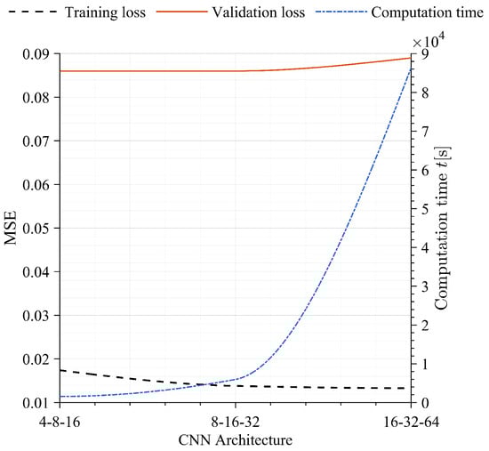
Figure 9. Optimization of the CNN architecture, showing the evolution of training and validation loss together with computational time for different layer configurations.

The CNN utilized filters with a size of 3 × 3, determining the area over which the filter operates, while larger filter sizes can potentially capture more information, they also escalate computational time, demand more memory and may yield less detailed information. For this study, a 3 × 3 filter was selected to prioritize detailed image information over global patterns, consistent with the objective of identifying localized areas of intensified port agitation and distinguishing them from calmer regions. For the stride, referring to the number of pixels by which the filter moves across the input image, a value of 1 was adopted, which is the standard setting in CNNs. A stride of 1 implies that the filter is applied to each pixel individually, ensuring that no pixel is skipped. This approach enables the network to capture patterns more accurately. Despite the associated increase in computational time, a stride of 1 was the best option due to its negligible impact on computational cost compared to the notable improvement in accuracy. Furthermore, the max pooling layers were configured with a size of 2 × 2, resulting in each 2 × 2 region being downsampled to a single maximum value. Similarly to the stride, increasing this value substantially raised the errors of the model. Consequently, a more conservative approach was adopted, acknowledging the increased demand for computational time and resources.

Among the different optimizers and activation functions available, Adam optimizer and RelU gave the best results. The final characteristics and representation of the model are presented in Table 3 and Figure 10. Once the hyperparameters of the model were optimized, it was trained, using 70% of the data samples to train the model and 30% of the data samples to validate it. The training time was 29 min 20 s.

Table 3. Optimized hyperparameters and performance metrics of the final model, including training and validation errors.

Hyperparameter	Value
N° epochs	100
Batch size	12
Learning rate	0.0005
Architecture FFNN	4–8
Architecture CNN	8–16–32
Convolutional filter size	$3\times 3$
MaxPooling size	$2\times 2$
Stride	1
Optimizer	Adam
Activation function	ReLU
Data partition	70% training, 30% validation
Error	Value
Training	0.0134
Validation	0.0800

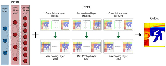
Figure 10. Final architecture of the deep learning model for port agitation. The hybrid structure integrates an FFNN branch, incorporating an input layer ($Hs,Tp,Dir$) and two hidden layers (neurons), with a CNN branch consisting of three convolutional layers (8, 16 and 32 filters of size 3 × 3) and max pooling layers (2 × 2).

4. Application and Validation of the Model

The deep learning model was successfully implemented and validated at the Port of Valencia, Spain. The results obtained by the proposed AI model (Figure 11b) were compared to those generated by MILDwave (Figure 11a), for 14 cases (30% of the total investigated cases), showcasing an almost similar prediction accuracy. Figure 11 demonstrates the remarkable consistency between the outcomes obtained from both approaches, for a representative case with a wave direction of $22.5^{°}$ N. Across all validation cases, the model achieved an MSE value of 0.08 per pixel, corresponding to an RMSE value of 0.283. Considering that pixel intensities are defined on a scale of 0 to 255, this RMSE value indicates an average deviation of significantly less than one intensity level per pixel, which is effectively negligible in terms of perceptual visual quality.

Figure 11. Disturbance coefficients ($k_d$) derived from the wave agitation study conducted in the Port of Valencia, Spain, for incident waves approaching from $22.5^{°}$ N, showing a comparison between MILDwave simulations and predictions from the developed AI model.

Once the model was validated, port agitation was studied under different wave conditions, based on present wave climate records and future projections. Wave periods from 5 s to 9 s and wave directions within sectors of $22.5^{°}$ were studied (Figure 12). It should be noted that the analysis was restricted to the directions in which the model was trained and validated, no testing was conducted for other directions. This represents one of the main limitations of the present study, as the model can only be applied within the $22.5^{°}$ sectors previously defined for training and validation. Application to other directions would require further investigation, including training and validation with a substantially larger set of images, an aspect not pursued in this work due to computational constraints.

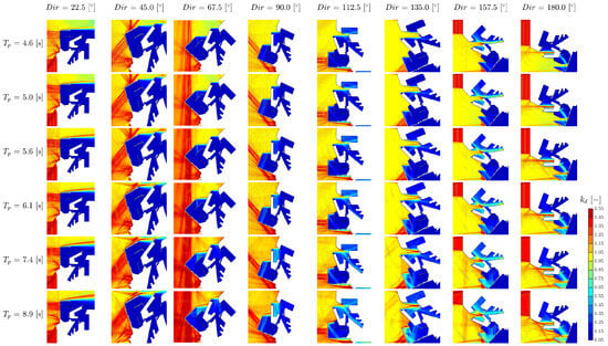
Figure 12. Port agitation in the Port of Valencia, Spain, under different wave conditions. Disturbance coefficients ($k_d$) values are shown from 0.05 (deep blue) to 1.55 (deep red), for peak wave periods ($T_p$) ranging from 4.6 s and 8.9 s and wave directions from $22.5^{°}$ to ${180}^{°}$.

Although the peak period currently in the Valencia area is more around 5–6 s, there are increasingly more weather events in the Mediterranean associated with much longer peak wave periods, around 10 s [57]. That is why it is important to analyze port agitation under these conditions. In fact, as seen in Figure 12, port agitation situations under longer periods are more critical than in the case of shorter periods. If the last row of the image matrix in Figure 12 corresponding to a period of 8.9 s is compared with the first row corresponding to a value of 4.6 s, it can be seen how the colors red and yellow predominate much more, corresponding to $k_d$ values greater than one, which means that wave height is amplified. When analyzing the wave direction, it is observed that operability issues may arise in the sector around ${90}^{°}$, corresponding to storms approaching from the East to the South (${180}^{°}$). In conclusion, the worst port agitation conditions would occur for periods of 8.9 s and directions of ${90}^{°}$, $112.5^{°}$, ${135}^{°}$, $157.5^{°}$ and ${180}^{°}$, which are the 5 images on the right side of the last row of Figure 13 (Cases 4.1, 5.1, 6.1, 7.1 and 8.1).

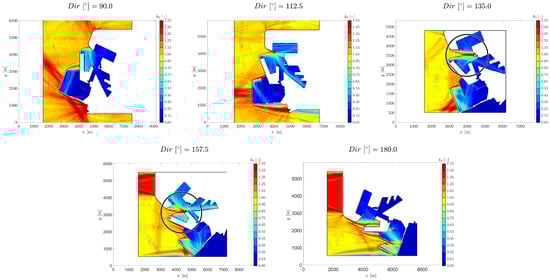
Figure 13. Worst-case disturbance coefficients ($k_d$) of port agitation in the Port of Valencia, Spain, for a peak wave period of $Tp=8.9$ s. The most critical conditions occur for wave directions of ${90}^{°}$–${180}^{°}$, particularly at ${135}^{°}$ and $157.5^{°}$, where localized wave amplification threatens port operability.

In general, the Port of Valencia is a sheltered and protected port, even for longer periods that are predicted to occur more frequently in the future. The situations of greater vulnerability occur for waves with directions of ${135}^{°}$ and $157.5^{°}$, which are highlighted by black solid circles in Figure 13. Under these conditions, the circled highlighted areas indicate regions where wave amplification may occur, potentially leading to operational issues within the port (Figure 13). Therefore, future research lines should study these cases in more detail and assess their potential impact on the operability of the Port of Valencia. Additionally, proposed solutions should be suggested if necessary.

5. Discussion

Most studies on port agitation have traditionally relied on numerical wave-propagation models [2,3], capable of reproducing wave dynamics with high fidelity, but at a high computational cost. Research on the Catalan coast [12,13], as well as the improved elliptic mild-slope model presented by Diaz-Hernandez et al. [32], demonstrate the field’s dependency to these numerically intensive techniques. Within the broader landscape of AI applications in seaports, AI-driven wave forecasting models are scarce [49]. For instance, Kankal and Yüksek [46] and López and Iglesias [47] employed artificial neural networks to transfer offshore wave climate to coastal locations, yet their emphasis was mainly on wave scaling and transformation rather than internal port agitation.

Thus, a novel hybrid deep learning model was developed based on existing ANNs, namely FFNNs and CNNs, as an efficient alternative to conventional numerical wave propagation models for predicting port agitation. This hybrid structure enables the integration of heterogeneous data sources, such as wave conditions and port geometry, enhancing the model’s ability to generalize across scenarios within predefined wave directional sectors.

Port of Valencia, Spain, was selected as a case study, where 48 numerical wave propagation simulations were generated using MILDwave, a mild-slope wave propagation model. The hybrid AI model was then trained using 70% of the simulated cases and validated using the remaining 30%. Despite the inherent simplifications of data-driven methods, the model achieved remarkable accuracy compared to MILDwave, showcasing an RMSE value of 0.283 per pixel, with pixel intensity values ranging from 0 to 255. These results highlight the suitability of the proposed surrogate model for applications requiring rapid or repeated predictions, including operational decision-making and preliminary climate change impact assessments.

In addition to computational efficiency, the trained AI model eliminates the need for extensive preprocessing tasks like calibration, bathymetry development and port layout adjustments. Once the AI model is trained, studying a new case only requires inputting the new wave conditions, whereas with numerical models, the entire model must be redeveloped. Additionally, as neural networks thrive on data, continuous usage enhances their precision, highlighting the importance of an iterative learning process. Furthermore, given the current situation of climate change, where climate and maritime patterns are shifting, it is necessary to study how these changes will affect ports, while existing studies predominantly focus on large ports due to their economic significance, small ports, most vulnerable to climate change, have been overlooked due to resource constraints. By reducing computational requirements, the methodologies proposed herein make it possible to extend research to these underserved areas, crucially contributing to our understanding and mitigation of port-related challenges in the face of climate change.

However, the model also has several limitations. It is currently restricted to the trained directional sectors ($22.5^{°}$ increments) and extrapolation to other directions is not yet feasible. The model’s performance may also be sensitive to the quality of input data and overfitting could occur if training data are insufficient or not representative. These limitations are inherent in surrogate and data-driven models, reflecting a trade-off between specificity and generalizability. Finally, the model is specifically trained for a case-specific site, namely the Port of Valencia, making it very sensitive to local morphology and bathymetry.

Despite these limitations, the findings from this site-specific study indicate that the Port of Valencia is expected to remain well-sheltered and resilient under future climate change conditions, except for wave directions between ${135}^{°}$ and $157.5^{°}$, where localized vulnerabilities and wave amplification may disrupt operations even in sheltered inner basins. For the wave direction of ${180}^{°}$, a particular sector of the port may also experience operational difficulties.

6. Conclusions

An AI-based deep neural network model has been developed to study port agitation, marking the first application of AI specifically dedicated to this problem. This work introduces a hybrid deep learning framework that combines CNNs, used for image analysis, with FFNNs, used to incorporate maritime climate conditions. By merging these two approaches, the model represents a novel attempt to address port agitation through image-based deep learning techniques.

The implementation of the proposed model significantly enhances computational efficiency, decreasing computation times relative to traditional wave propagation models by a factor ranging from four to ten, depending on the scenario and model type employed. The accuracy of the AI model was assessed against MILDwave, a mild-slope wave propagation model, demonstrating very low error levels. Further validation using additional wave propagation models governed by different phase-resolving equations could help identify potential sources of misprediction and enhance the overall reliability of the proposed approach.

The main limitation of this study lies in its applicability to a site-specific location, namely the Port of Valencia, while even within this localized context, a secondary limitation concerns its restriction to the trained and validated directional sectors. Expanding the applicability of the model to other ports and directions would require the incorporation of additional cases and a substantially larger number of images, which was not feasible within the scope of this work due to computational and resource constraints. This study primarily aims to demonstrate an AI-based methodological framework for port agitation analysis and to illustrate its applicability to real marine infrastructures. Future research should therefore prioritize extending the model to cover all directional sectors, thereby ensuring full applicability in the context of Valencia. Subsequently, it should aim to be trained on different spatial and temporal patterns, enabling its generalization and adaptation to other site locations. Achieving this objective will demand a considerable investment in both time and computational resources to manage and process the complete datasets. In parallel, further studies should explore strategies for optimizing memory usage and reducing computational overhead in large-scale image processing. Such advances would not only enable the development of a fully generalized model but also enhance its scalability and applicability to broader geographical and environmental contexts.

Nevertheless, the findings from this site-specific study indicate that the Port of Valencia is expected to remain well-sheltered and resilient under future climate change conditions, except for wave directions from the southeast to the south sector, where localized vulnerabilities and wave amplification may hinder operations. Continued development of the AI model could provide decision-makers at the Port of Valencia with a fast-response tool to simulate the intra-port wave field for operational maneuverability or short-notice storm forecasts, as well as in assessing the risks and costs of future investment strategies under climate-induced wave conditions.

References

- Losada, M.A.; Baquerizo, A.; Ortega-Sanchez, M.; Avila, A. Coastal Evolution, Sea Level, and Assessment of Intrinsic Uncertainty. J. Coast. Res. 2011, SI59, 218–228. [Google Scholar] [CrossRef]
- Masselink, G.; Hughes, M. An Introduction to Coastal Processes and Geomorphology; Routledge: London, UK, 2003. [Google Scholar] [CrossRef]
- Hinkel, J.; Lincke, D.; Vafeidis, A.T.; Perrette, M.; Nicholls, R.J.; Tol, R.S.J.; Marzeion, B.; Fettweis, X.; Ionescu, C.; Levermann, A. Coastal Flood Damage and Adaptation Costs under 21st Century Sea-Level Rise. Proc. Natl. Acad. Sci. USA 2014, 111, 3292–3297. [Google Scholar] [CrossRef]
- Luijendijk, A.; Hagenaars, G.; Ranasinghe, R.; Baart, F.; Donchyts, G.; Aarninkhof, S. The State of the World’s Beaches. Sci. Rep. 2018, 8, 6641. [Google Scholar] [CrossRef] [PubMed]
- Mentaschi, L.; Vousdoukas, M.I.; Pekel, J.-F.; Voukouvalas, E.; Feyen, L. Global Long-Term Observations of Coastal Erosion and Accretion. Sci. Rep. 2018, 8, 12876. [Google Scholar] [CrossRef] [PubMed]
- Garcia-Alonso, L.; Moura, T.G.Z.; Roibas, D. The Effect of Weather Conditions on Port Technical Efficiency. Mar. Policy 2020, 113, 103816. [Google Scholar] [CrossRef]
- International Maritime Organization. International Shipping Facts and Figures—Information Resources on Trade, Safety, Security, Environment; Maritime Knowledge Centre, IMO: London, UK, 2012. [Google Scholar]
- UNCTAD. Review of Maritime Transport; United Nations Publication: Geneva, Switzerland, 2019. [Google Scholar]
- UNCTAD. Climate Change Impacts and Adaptation: A Challenge for Global Ports. Available online: https://unctad.org/system/files/official-document/dtltlb2011d2_en.pdf (accessed on 18 November 2021).
- Portillo Juan, N.; Negro Valdecantos, V.; del Campo, J.M. Analysis of Monthly Recorded Climate Extreme Events and Their Implications on the Spanish Mediterranean Coast. Water 2022, 14, 3453. [Google Scholar] [CrossRef]
- Cramer, W.; Guiot, J.; Fader, M.; Garrabou, J.; Gattuso, J.-P.; Iglesias, A.; Lange, M.A.; Lionello, P.; Llasat, M.C.; Paz, S.; et al. Climate Change and Interconnected Risks to Sustainable Development in the Mediterranean. Nat. Clim. Change 2018, 8, 972–980. [Google Scholar] [CrossRef]
- Casas-Prat, M.; Sierra, J.P. Trend Analysis of Wave Storminess: Wave Direction and Its Impact on Harbour Agitation. Nat. Hazards Earth Syst. Sci. 2010, 10, 2327–2340. [Google Scholar] [CrossRef]
- Casas-Prat, M.; Sierra, J.P. Trend Analysis of Wave Direction and Associated Impacts on the Catalan Coast. Clim. Change 2012, 115, 667–691. [Google Scholar] [CrossRef]
- Sierra, J.P.; Casas-Prat, M.; Virgili, M.; Moesso, C.; Sánchez-Arcilla, A. Impacts on Wave-Driven Harbour Agitation Due to Climate Change in Catalan Ports. Nat. Hazards Earth Syst. Sci. 2015, 15, 1695–1709. [Google Scholar] [CrossRef]
- Becker, A.; Inoue, S.; Fischer, M.; Schwegler, B. Climate Change Impacts on International Seaports: Knowledge, Perceptions, and Planning Efforts among Port Administrators. Clim. Change 2012, 110, 5–29. [Google Scholar] [CrossRef]
- Messner, S.F.; Moran, L.; Reub, G.; Campbell, J. Climate Change and Sea Level Rise Impacts at Ports and a Consistent Methodology to Evaluate Vulnerability and Risk. WIT Trans. Ecol. Environ. 2013, 169, 141–153. [Google Scholar] [CrossRef]
- Nursey-Bray, M.; Blackwell, B.; Brooks, B.; Campbell, M.L.; Goldsworthy, L.; Pateman, H.; Rodrigues, I.; Roome, M.; Wright, J.T.; Francis, J.; et al. Vulnerabilities and Adaptation of Ports to Climate Change. J. Environ. Plan. Manag. 2013, 56, 1021–1045. [Google Scholar] [CrossRef]
- Reckien, D.; Flacke, J.; Olazabal, M.; Heidrich, O. The Influence of Drivers and Barriers on Urban Adaptation and Mitigation Plans—An Empirical Analysis of European Cities. PLoS ONE 2015, 10, e0135597. [Google Scholar] [CrossRef]
- Sierra, J.P.; Casas-Prat, M. Analysis of Potential Impacts on Coastal Areas Due to Changes in Wave Conditions. Clim. Change 2014, 124, 861–876. [Google Scholar] [CrossRef]
- Hardy, R.D.; Nuse, B.L. Global Sea-Level Rise: Weighing Country Responsibility and Risk. Clim. Change 2016, 137, 333–345. [Google Scholar] [CrossRef]
- Sánchez-Arcilla, A.; García-León, M.; Gracia, V.; Devoy, R.; Stanica, A.; Gault, J. Managing Coastal Environments under Climate Change: Pathways to Adaptation. Sci. Total Environ. 2016, 572, 1336–1352. [Google Scholar] [CrossRef] [PubMed]
- Mutombo, K.; Ölçer, A. Towards Port Infrastructure Adaptation: A Global Port Climate Risk Analysis. WMU J. Marit. Aff. 2017, 16, 161–173. [Google Scholar] [CrossRef]
- Prahl, B.F.; Boettle, M.; Costa, L.; Kropp, J.P.; Rybski, D. Damage and Protection Cost Curves for Coastal Floods within the 600 Largest European Cities. Sci. Data 2018, 5, 180034. [Google Scholar] [CrossRef] [PubMed]
- Abadie, L.; Galarraga, I.; Markandya, A.; Sainz de Murieta, E. Risk Measures and the Distribution of Damage Curves for 600 European Coastal Cities. Environ. Res. Lett. 2019, 14, 074017. [Google Scholar] [CrossRef]
- Christodoulou, A.; Christidis, P.; Demirel, H. Sea-Level Rise in Ports: A Wider Focus on Impacts. Marit. Econ. Logist. 2019, 21, 482–496. [Google Scholar] [CrossRef]
- Hanson, S.E.; Nicholls, R.J. Demand for Ports to 2050: Climate Policy, Growing Trade and the Impacts of Sea-Level Rise. Earth’s Future 2020, 8, e2020EF001543. [Google Scholar] [CrossRef]
- Abadie, L.M.; Sainz de Murieta, E.; Galarraga, I. The Costs of Sea-Level Rise: Coastal Adaptation Investments vs. Inaction in Iberian Coastal Cities. Water 2020, 12, 1220. [Google Scholar] [CrossRef]
- Izaguirre, C.; Losada, I.J.; Camus, P.; González-Lamuño, P.; Stenek, V. Seaport Climate Change Impact Assessment Using a Multi-Level Methodology. Marit. Policy Manag. 2020, 47, 544–557. [Google Scholar] [CrossRef]
- Izaguirre, C.; Losada, I.J.; Camus, P.; Vigh, J.L.; Stenek, V. Climate Change Risk to Global Port Operations. Nat. Clim. Change 2021, 11, 14–20. [Google Scholar] [CrossRef]
- Wiegel, M.; de Boer, W.; van Koningsveld, M.; van der Hout, A.; Reniers, A. Global Mapping of Seaport Operability Risk Indicators Using Open-Source Metocean Data. J. Mar. Sci. Eng. 2021, 9, 695. [Google Scholar] [CrossRef]
- Leon-Mateos, F.; Sartal, A.; Lopez-Manuel, L.; Quintas, M.A. Adapting Our Sea Ports to the Challenges of Climate Change: Development and Validation of a Port Resilience Index. Mar. Policy 2021, 130, 104573. [Google Scholar] [CrossRef]
- Diaz-Hernandez, G.; Fernandez, B.R.; Romano-Moreno, E.; Lara, J.L. An Improved Model for Fast and Reliable Harbour Wave Agitation Assessment. Coast. Eng. 2021, 170, 104011. [Google Scholar] [CrossRef]
- Romano-Moreno, E.; Diaz-Hernandez, G.; Lara, J.L.; Tomás, A.; Jaime, F. Wave Downscaling Strategies for Practical Wave Agitation Studies in Harbours. Coast. Eng. 2022, 175, 104140. [Google Scholar] [CrossRef]
- Romano-Moreno, E.; Diaz-Hernandez, G.; Tomás, A.; Lara, J.L. Multimodal Harbor Wave Climate Characterization Based on Wave Agitation Spectral Types. Coast. Eng. 2023, 180, 104271. [Google Scholar] [CrossRef]
- Sánchez-Arcilla, A.; Pau Sierra, J.; Brown, S.; Casas-Prat, M.; Nicholls, R.J.; Lionello, P.; Conte, D. A Review of Potential Physical Impacts on Harbours in the Mediterranean Sea under Climate Change. Reg. Environ. Change 2016, 16, 2471–2484. [Google Scholar] [CrossRef]
- Sierra, J.P.; Garcia-Leon, M.; Gracia, V.; Sanchez-Arcilla, A. Green Measures for Mediterranean Harbours under a Changing Climate. Proc. Inst. Civ. Eng.-Marit. Eng. 2017, 170, 55–66. [Google Scholar] [CrossRef]
- Diaz-Hernandez, G.; Lara, J.L.; Losada, I.J. Extended Long Wave Hindcast inside Port Solutions to Minimize Resonance. J. Mar. Sci. Eng. 2016, 4, 9. [Google Scholar] [CrossRef]
- Laxe, F.G.; Bermúdez, F.M.; Palmero, F.M.; Novo-Corti, I. Assessment of Port Sustainability through Synthetic Indexes: Application to the Spanish Case. Mar. Pollut. Bull. 2017, 119, 220–225. [Google Scholar] [CrossRef] [PubMed]
- Velasco, M.; Russo, B.; Cabello, A.; Termes, M.; Sunyer, D.; Malgrat, P. Assessment of the Effectiveness of Structural and Nonstructural Measures to Cope with Global Change Impacts in Barcelona. J. Flood Risk Manag. 2018, 11, S55–S68. [Google Scholar] [CrossRef]
- Vinet, F.; Bigot, V.; Petrucci, O.; Papagiannaki, K.; Llasat, M.C.; Kotroni, V.; Boissier, L.; Aceto, L.; Grimalt, M.; Llasat-Botija, M.; et al. Mapping Flood-Related Mortality in the Mediterranean Basin: Results from the MEFF v2.0 DB. Water 2019, 11, 2196. [Google Scholar] [CrossRef]
- Gracia, V.; Sierra, J.P.; Gomez, M.; Pedrol, M.; Sampe, S.; Garcia-Leon, M.; Gironella, X. Assessing the Impact of Sea Level Rise on Port Operability Using LiDAR-Derived Digital Elevation Models. Remote Sens. Environ. 2019, 232, 111318. [Google Scholar] [CrossRef]
- Sierra, J.P.; Genius, A.; Lionello, P.; Mestres, M.; Mosso, C.; Marzo, L. Modelling the Impact of Climate Change on Harbour Operability: The Barcelona Port Case Study. Ocean Eng. 2017, 141, 64–78. [Google Scholar] [CrossRef]
- Camus, P.; Tomás, A.; Diaz-Hernandez, G.; Rodriguez, B.; Izaguirre, C.; Losada, I.J. Probabilistic Assessment of Port Operation Downtimes under Climate Change. Coast. Eng. 2019, 147, 12–25. [Google Scholar] [CrossRef]
- Jebbad, R.; Sierra, J.P.; Mosso, C.; Mestres, M.; Sánchez-Arcilla, A. Assessment of Harbour Inoperability and Adaptation Cost Due to Sea Level Rise: Application to the Port of Tangier-Med (Morocco). Appl. Geogr. 2022, 138, 102623. [Google Scholar] [CrossRef]
- Sierra, J.; Sánchez-Arcilla, A.; Gironella, X.; Garcia, V.; Altomare, C.; Mösso, C.; González-Marco, D.; Gomez, J.; Barceló, M.; Barahona, C. Impact of Climate Change on Berthing Areas in Ports of the Balearic Islands: Adaptation Measures. Front. Mar. Sci. 2023, 10, 1124763. [Google Scholar] [CrossRef]
- Kankal, M.; Yüksek, Ö. Artificial Neural Network Approach for Assessing Harbor Tranquility: The Case of Trabzon Yacht Harbor, Turkey. Appl. Ocean Res. 2012, 38, 23–31. [Google Scholar] [CrossRef]
- López, M.; Iglesias, G. Artificial Neural Networks Applied to Port Operability Assessment. Ocean Eng. 2015, 109, 298–307. [Google Scholar] [CrossRef]
- Portillo Juan, N.; Olalde Rodríguez, J.; Negro Valdecantos, V.; Iglesias, G. Data-Driven and Physics-Based Approach for Wave Downscaling: A Comparative Study. Ocean Eng. 2023, 285, 115380. [Google Scholar] [CrossRef]
- Liu, X.; Yuen, K.F. A systematic review on artificial intelligence applications in seaports—A network analysis approach. Expert Syst. Appl. 2025, 289, 128309. [Google Scholar] [CrossRef]
- Chondros, M.K.; Metallinos, A.S.; Papadimitriou, A.G. Enhanced mild-slope wave model with parallel implementation and artificial neural network support for simulation of wave disturbance and resonance in ports. J. Mar. Sci. Eng. 2024, 12, 281. [Google Scholar] [CrossRef]
- Zheng, Z.; Ma, X.; Ma, Y.; Dong, G. Wave estimation within a port using a fully nonlinear Boussinesq wave model and artificial neural networks. Ocean Eng. 2020, 216, 108073. [Google Scholar] [CrossRef]
- Zheng, Z.; Ma, X.; Huang, X.; Ma, Y.; Dong, G. Wave forecasting within a port using WAVEWATCH III and artificial neural networks. Ocean Eng. 2022, 255, 111475. [Google Scholar] [CrossRef]
- Huang, X.; Tang, J.; Shen, Y. Long time series of ocean wave prediction based on PatchTST model. Ocean Eng. 2024, 301, 117572. [Google Scholar] [CrossRef]
- Zang, T.; Zou, J.; Li, Y.; Qiu, Z.; Wang, B.; Cui, C.; Li, Z.; Hu, T.; Guo, Y. Development and evaluation of a short-term ensemble forecasting model on sea surface wind and waves across the Bohai and Yellow Sea. Atmosphere 2024, 15, 197. [Google Scholar] [CrossRef]
- Wang, X.; Jiang, H. Physics-guided deep learning for skillful wind–wave modeling. Sci. Adv. 2024, 10, eadr3559. [Google Scholar] [CrossRef]
- López, M.; Iglesias, G. Artificial Intelligence for Estimating Infragravity Energy in a Harbour. Ocean Eng. 2013, 57, 56–63. [Google Scholar] [CrossRef]
- Portillo Juan, N.; Negro Valdecantos, V.; del Campo, J.M. Review of the Impacts of Climate Change on Ports and Harbours and Their Adaptation in Spain. Sustainability 2022, 14, 7507. [Google Scholar] [CrossRef]
- Puertos del Estado. Oceanografía. Registros Históricos de Oleaje. Available online: https://www.puertos.es/es-es/oceanografia/Paginas/portus.aspx (accessed on 19 September 2022).
- Portillo Juan, N.; Negro Valdecantos, V. A Novel Model for the Study of Future Maritime Climate Using Artificial Neural Networks and Monte Carlo Simulations under the Context of Climate Change. Ocean Model. 2024, 190, 102384. [Google Scholar] [CrossRef]
- Booij, N.; Ris, R.C.; Holthuijsen, L.H. A Third-Generation Wave Model for Coastal Regions: 1. Model Description and Validation. J. Geophys. Res. Oceans 1999, 104, 7649–7666. [Google Scholar] [CrossRef]
- GEBCO. General Bathymetric Chart of the Oceans. Available online: https://www.gebco.net/ (accessed on 7 January 2023).
- Komen, G.J.; Hasselmann, S.; Hasselmann, K. On the Existence of a Fully Developed Wind-Sea Spectrum. J. Phys. Oceanogr. 1984, 14, 1271–1285. [Google Scholar] [CrossRef]
- Battjes, J.A.; Janssen, J.P.F.M. Energy Loss and Set-Up Due to Breaking of Random Waves. In Coastal Engineering 1978; ASCE: Hamburg, Germany, 1978; pp. 569–587. [Google Scholar] [CrossRef]
- Hasselmann, K.; Barnett, T.; Bouws, E.; Carlson, H.; Cartwright, D.; Enke, K.; Ewing, J.; Gienapp, H.; Hasselmann, D.; Kruseman, P.; et al. Measurements of Wind-Wave Growth and Swell Decay during the Joint North Sea Wave Project (JONSWAP). Dtsch. Hydrogr. Z. 1973, 8, 1–95. [Google Scholar]
- Troch, P. MILDwave—A Numerical Model for Propagation and Transformation of Linear Water Waves; Internal Report; Department of Civil Engineering, Ghent University: Ghent, Belgium, 1998. [Google Scholar]
- Radder, A.C.; Dingemans, M.W. Canonical Equations for Almost Periodic, Weakly Nonlinear Gravity Waves. Wave Motion 1985, 7, 473–485. [Google Scholar] [CrossRef]
- Portillo Juan, N.; Negro Valdecantos, V. Review of the Application of Artificial Neural Networks in Ocean Engineering. Ocean Eng. 2022, 259, 111947. [Google Scholar] [CrossRef]
- Yuan, F.; Xu, Y.; Li, Q.; Mostafavi, A. Spatio–temporal graph convolutional networks for road network inundation status prediction during urban flooding. Comput. Environ. Urban Syst. 2022, 97, 101870. [Google Scholar] [CrossRef]
- Ruscio, F.; Costanzi, R.; Gracias, N.; Quintana, J.; Garcia, R. Autonomous Boundary Inspection of Posidonia oceanica Meadows Using an Underwater Robot. Ocean Eng. 2023, 283, 114988. [Google Scholar] [CrossRef]
- Bento, P.M.R.; Pombo, J.A.N.; Mendes, R.P.G.; Calado, M.R.A.; Mariano, S.J.P.S. Ocean Wave Energy Forecasting Using Optimised Deep Learning Neural Networks. Ocean Eng. 2021, 219, 108372. [Google Scholar] [CrossRef]
- Yao, Y.; Yang, Y.; Wang, Y.; Zhao, X. Artificial Intelligence-Based Hull Structural Plate Corrosion Damage Detection and Recognition Using Convolutional Neural Network. Appl. Ocean Res. 2019, 90, 101823. [Google Scholar] [CrossRef]
- Abadi, M.; Agarwal, A.; Barham, P.; Brevdo, E.; Chen, Z.; Citro, C.; Corrado, G.S.; Davis, A.; Dean, J.; Devin, M.; et al. TensorFlow: Large-Scale Machine Learning on Heterogeneous Distributed Systems. arXiv 2016, arXiv:1603.04467. [Google Scholar] [CrossRef]
- Chollet, F. Keras. 2015. Available online: https://keras.io (accessed on 8 December 2023).
- Dang, K.B.; Dang, V.B.; Bui, Q.T.; Nguyen, V.V.; Pham, T.P.N.; Ngo, V.L. A Convolutional Neural Network for Coastal Classification Based on ALOS and NOAA Satellite Data. IEEE Access 2020, 8, 11824–11839. [Google Scholar] [CrossRef]
Disclaimer/Publisher’s Note: The statements, opinions and data contained in all publications are solely those of the individual author(s) and contributor(s) and not of MDPI and/or the editor(s). MDPI and/or the editor(s) disclaim responsibility for any injury to people or property resulting from any ideas, methods, instructions or products referred to in the content. |
© 2025 by the authors. Licensee MDPI, Basel, Switzerland. This article is an open access article distributed under the terms and conditions of the Creative Commons Attribution (CC BY) license (https://creativecommons.org/licenses/by/4.0/).