Routing a Fleet of Drones from a Base Station for Emission Detection of Moving Ships by Genetic Algorithm

Abstract

A fleet of drones is considered in the routing problems with an offshore drone base station, considering the simultaneous movements of drones and ships. A model, entitled meeting model, between a drone and a moving ship is devised, and an extended model is developed based on the vehicle routing problem model. A genetic algorithm based on a sequential insert heuristic (SIH) is designed to solve the model as a holistic framework with two strategies to determine the sequential assignments of ships to drones, namely, the $\mathrm{D}\mathrm{r}\mathrm{o}\mathrm{n}\mathrm{e}\mathrm{B}\mathrm{y}\mathrm{D}\mathrm{r}\mathrm{o}\mathrm{n}\mathrm{e},$ and $\mathrm{S}\mathrm{h}\mathrm{i}\mathrm{p}\mathrm{B}\mathrm{y}\mathrm{S}\mathrm{h}\mathrm{i}\mathrm{p}$ strategies. The proposed models and solution algorithms are demonstrated and verified by experiments. Numerical studies show that the $\mathrm{D}\mathrm{r}\mathrm{o}\mathrm{n}\mathrm{e}\mathrm{B}\mathrm{y}\mathrm{D}\mathrm{r}\mathrm{o}\mathrm{n}\mathrm{e}$ strategy can overperform the $\mathrm{S}\mathrm{h}\mathrm{i}\mathrm{p}\mathrm{B}\mathrm{y}\mathrm{S}\mathrm{h}\mathrm{i}\mathrm{p}$ strategy regarding traveling distances. In addition, when considering the simultaneous movement of the ship and drone, improving the drone flying speeds can reduce the flying time of drones rather than optimizing the ship’s moving speed. The managerial implications and possible extensions are discussed based on modeling and experimental studies.

1. Introduction

As an essential component of logistics transportation, maritime transportation plays a crucial role in connecting global markets and promoting international trade. Global maritime cargo trade is expected to nearly triple between 2020 and 2050 [1]. As a result, the growth in shipping demand is causing shipping pollution concerns. According to the findings of the International Maritime Organization, the shipping industry’s carbon dioxide emissions constitute approximately 2.2% of worldwide total emissions. Ship fuel combustion also produces nitrogen oxides, sulfur oxides, and other pollutants. The oxides and pollutants negatively impact the environment and human health [2]. The pollutants emitted from ships at high altitudes can spread to an area with air currents, causing more severe impacts on the ground and atmosphere, especially in Port City. Therefore, the International Maritime Organization (IMO) institutes Emission Control Areas (ECAs) globally to regulate maritime emissions.

ECA aims to significantly reduce ship pollutant emissions and promote a green and sustainable shipping industry. Within ECAs, maritime regulations mandate the utilization of fuels with a sulfur content that does not exceed a specified threshold. Nonetheless, the absence of a cost–benefit for low sulfur oil compared to heavy oil leads numerous shipping enterprises and vessel owners to favor heavy oil for marine fuel. Consequently, the monitoring of ship emissions in ECAs becomes critically essential. The traditional detection method is to take samples on board, send them to a third party for inspection, or use a fast detector for detection. However, the operation has low detection efficiency and is complex. Hence, innovative emission detection and regulation methods are among the most essential ways to control shipping pollution. Among them, onboard drone-based sniffing technology can realize fast and remote online monitoring and can be used as a feasible and reliable means of pollution monitoring. However, drones’ initial acquisition costs and ongoing maintenance are relatively high. As a result, reasonable scheduling and optimizing the routes for drones should be developed to ensure cost-effectiveness.

This study contributes to the related studies in the following three aspects. First, we consider the simultaneous movements of drones and ships according to their respective moving directions and speeds and propose a meeting model to optimize the catch-up time during drone ship emissions. Second, since a fleet of drones’ detection scenario for ships is much like the classical VRP, we formulated the routing problem based on VRP models. However, the customer points visited by the vehicles in the VRP are stationary while the ships are moving. The general VRP models cannot be fully adapted to this problem. We extend the VRP models by proposing an extended model considering “moving customers”. Finally, we develop a sequential insert heuristic (SIH) and SIH-based bi-stage solution algorithm to compute the drones’ and ships’ meeting times and positions and then create an SIH-based genetic algorithm to calculate the visiting order of ships by the drone for emissions detection.

The rest of the sections are organized as follows. Section 2 reviews the related studies on ECA, ship emission detection, and drone routing problems. Section 3 introduces the problem and investigates two routing modes, the TSP-based and VRP-based modes. Section 4 formulates the mathematical models. Section 5 presents a genetic algorithm based on a sequential insert heuristic algorithm. Then, we conduct a series of numerical experiments to examine the proposed models and algorithms and discuss the managerial implications in Section 6. We conclude this study in Section 7.

2. Related Studies

This study featured the drone routing problem inspired by drone applications in emission detection in emission control areas (ECAs).

2.1. Emission Control Area

An ECA regulates the release of harmful gases from ships, aiming to diminish the emissions of sulfur dioxide, nitrogen oxides, and particulate matter regarding the effects of ship emissions on human health and the environment [3]. Data from the IMO indicate that the implementation of ECAs in Europe has resulted in a 60% decrease in sulfur dioxide emissions from ships [4]. Implementing ECA has driven the development of new technologies, such as exhaust gas scrubbers and liquefied natural gas (LNG), which can effectively control ship emissions.

Table 1 summarizes the research on ECA in terms of the research questions, methods, and corresponding regions or ports. ECA is a universal emission control solution; so, most governments and ports have taken it as a policy-making and administration tool. The research in Table 1 investigated various features, including ECA formation, impact assessment, scheduling optimization based on ECA, and stakeholder behaviors. Four methods are used in the research: data-driven [5], mathematical analysis [6], optimization [7], and evaluation methods [8]. In Table 1, emission control is significant, and various technologies were applied. Drones should emerge as new devices for ECA management, challenging drone scheduling, and routing problems.

Table 1. Pioneering studies on ECA.

Study	Research Problem	Method	Region/Port
[9]	Design China’s domestic ECA	BLP	China
[6]	The accomplishment of the ECA program development	A	China
[10]	Assess noxious gases of ship operations in a potential ECA	D	Incheon Port
[11]	The spatial relationship between the net benefit and the size of ECA	Simulation	China
[7]	Locate ECA to minimize the impacts of Sulfur emissions on human health	MILP	China, Africa
[12]	Dual environmental effects of ECA and reduced speed zones	MILP	Pacific Ocean
[5]	Investigate the heterogeneity of the ECA policy effectiveness	D	Yangtze River Delta
[8]	Examine whether ECA regulations impact the efficiency of ports	DEA	European Union, North America
[13]	Impact of Sulfur ECA on port state control’s inspection outcome	A	-
[4]	Influence of sulfur emission control areas on particulate matter emission	A	China
[14]	Optimize ship route and speed with ECA simultaneously	A	-
[15]	Global impacts of ECA	A	Asia, Europe
[16]	Decision on liner shipping considering ECA regulations	MINP	North America
[17]	Analyze the ship’s response strategy to ECA	MINP	North America

Note: A = Mathematical analytical model; BLP = Bi-level program; D = Statistics or other data-driven analysis; DEA = Data envelopment analysis; H = Heuristics; MILP = Mixed-integer linear program; MINP = Mixed-integer nonlinear program.

2.2. Ship Emission Detection

Ship emission detection technologies play a critical role in reducing the impact of ship emissions on the environment and public health [3]. Ship emission detection technologies are still developing, and future research should focus on improving the technology’s accuracy, efficiency, and cost-effectiveness [18]. Drones equipped with sniffing technology have been tested and applied to detect atmospheric pollution on ships. Using drones for ship emission detection can achieve remote, online, and real-time detection. It is more efficient, flexible, and convenient than conventional detection methods.

Table 2 summarizes some groundbreaking research on ship emission detection in three areas: the research problem, research method, and detection method. The research problem includes ship emission detection methods, detection accuracy optimization, and detection effectiveness evaluation. Research methods related to ship detection issues include neural networks [18], simulation analysis [19], machine learning [20], optimization [21], and utilizing data such as Automatic Identification System (AIS) data [22], satellite images, and videos. Detection methods involve remote sensing, onboard measurement [23], and imaging pattern recognition [24]. This study applied a fleet of drones to ship emission detection and investigated the scheduling and routing problem of drones equipped with specialized emission detection devices.

Table 2. Pioneering studies on Ship emission detection.

Study	Research Problem	Detection	Solution
[18]	Individual ship pollution or ship plume evaluation	Onboard	NN
[20]	A big data analytics framework for ship performance monitoring	Onboard	ML
[25]	Apply an energy consumption approach to estimate container ship emissions	Onboard	EA
[22]	A method evaluating emissions in detailed	Onboard	EA
[23]	Precise identification of carbon emission hotspot areas and ship types in ports	Onboard	D
[19]	Monitor the SO2 concentration in ship exhausts	Imaging	S
[26]	Estimate SO2, CO2, and NO concentrations of exhaust gas by imaging methods	Imaging	NN
[27]	Investigating the impacts of satellite fire observation accuracy on the top-down nitrogen oxide emission estimation in northeastern Asia.	RS	D
[21]	Develop a marine diesel SOX online detection system	RS	H
[28]	Remotely detect sulfur contents in fuel oil used by ships in ECA	RS	S
[24]	Detect NO2 pollution plumes from ships with the TROPOMI/S5P satellite sensors.	RS	D

Note: RS = Remote sensing; D = Statistics or other data-driven methods; DFT = Data field theory; DL = Deep learning; EA = Empirical analysis; H = Heuristics; ML = Machine learning; NN = Neural network; S = Simulation.

2.3. Drone Routing Problem

Several complex stages are involved during ship emission detection, including law enforcement personnel boarding, document verification, fuel sampling, and actual detection [29]. Drones offer numerous benefits, including their high mobility, precise information gathering, and prompt data transmission, making them widely applicable in various fields [30]. Drones can detect and monitor ship emissions in the emission control area, constrained by energy consumption and cost [31]. Most importantly, drones used for ship emission detection must handle the simultaneous movements of ships, which is a distinct feature in the literature and challenges the existing routing models and solution algorithms.

Most of the literature formulates the drone routing problem as a mixed-integer linear programming (MILP) to determine the task assignment and the visited orders for each drone. Table 3 lists the research on drone routing problems under various scenarios. The VRPs are NP-hard; so, general MILP solvers can only solve small-scale tasks. Hence, to solve medium- and large-scale tasks, researchers usually develop heuristics [32] (e.g., greedy, neighborhood search), a metaphor approach [33,34] (e.g., genetic algorithm, Ant colony optimization), and a decomposition-based algorithm [35] (e.g., Branch-and-Cut, Branch-and-Price).

In terms of application, the delivery and distribution (mainly including emergency [36], last-mile delivery [33], and monitoring [37]) can inspire the model and algorithm developments. We can observe distinct features of the drone scheduling problems: endurance and collaborative delivery with trucks [38]. This study formulated the drone routing problem based on VRP modes and their concepts. In ship emission detection, the tasks performed by a fleet of drones and a drone may visit more than one ship.

Applying drones to ship emission detection has the characteristics of a basic VRP. Specifically, a drone flies from a drone base station to the ship, whose position can be determined by the AIS receivers connected with the station [22]. Namely, the ship to be detected corresponds to the customer in a typical VRP. As a difference, the ship is not a stationary object but moves with time. These distinct features challenge the existing models and solution algorithms studied in Table 3. To model the proposed problem, we review the related VRP with drones to provide a fruitful methodological reference.

Table 3. Pioneering studies on drone routing problems.

Study	Application Scenario	TSP/VRP Variance	Model	Algorithm
[39]	Last-mile package delivery	VRP with drones	MILP	VNS + TS
[32]	Truck–drone collaborative delivery	Parallel TSP	MILP	H
[31]	Truck–drone collaborative delivery	Multi-trip VRP with time windows	MILP	B&C
[40]	Truck–drone collaborative delivery	Multi-visit VRP	Analytical	H
[41]	Mothership-drone coordination	VRP with drones	MISOCP	MH
[35]	Last-mile package delivery	TSP with drones	MILP	B&P
[42]	Last-mile package delivery	VRP with drones	MILP	B&C
[36]	Emergency delivery	VRP with drones	Analytical	-
[43]	Delivery	VRP with drones	MILP	ACO
[44]	Island delivery	VRP with drones	RO	-
[45]	Truck–multi-drone team delivery	TSP with multiple flying sidekicks	Reasoning	ML
[33]	Last-mile package delivery	VRP with backhauls	MILP	SA + VNS
[38]	Truck–drone collaborative delivery	VRP with time-dependent road travel time	MILP	H
[46]	Surveillance	Nested VRP	MIQCP	NS

Note: ACO = Ant colony optimization; B&B = Branch-and-Bound; B&C = Branch-and-Cut; B&P = Branch-and-Price; H = Heuristic; MH = Math-heuristic; MILP = Mixed-integer linear program; MIQCP = Mixed-integer quadratically constrained programming; MISOCP = Mixed-integer second-order cone programming; ML = Machine learning; NS = Neighborhood search; RO = Robust optimization; SA = Simulated annealing; TS = Tabu search; VNS = Variable neighborhood search.

Table 3. Pioneering studies on drone routing problems.

Study	Application Scenario	TSP/VRP Variance	Model	Algorithm
[39]	Last-mile package delivery	VRP with drones	MILP	VNS + TS
[32]	Truck–drone collaborative delivery	Parallel TSP	MILP	H
[31]	Truck–drone collaborative delivery	Multi-trip VRP with time windows	MILP	B&C
[40]	Truck–drone collaborative delivery	Multi-visit VRP	Analytical	H
[41]	Mothership-drone coordination	VRP with drones	MISOCP	MH
[35]	Last-mile package delivery	TSP with drones	MILP	B&P
[42]	Last-mile package delivery	VRP with drones	MILP	B&C
[36]	Emergency delivery	VRP with drones	Analytical	-
[43]	Delivery	VRP with drones	MILP	ACO
[44]	Island delivery	VRP with drones	RO	-
[45]	Truck–multi-drone team delivery	TSP with multiple flying sidekicks	Reasoning	ML
[33]	Last-mile package delivery	VRP with backhauls	MILP	SA + VNS
[38]	Truck–drone collaborative delivery	VRP with time-dependent road travel time	MILP	H
[46]	Surveillance	Nested VRP	MIQCP	NS

Note: ACO = Ant colony optimization; B&B = Branch-and-Bound; B&C = Branch-and-Cut; B&P = Branch-and-Price; H = Heuristic; MH = Math-heuristic; MILP = Mixed-integer linear program; MIQCP = Mixed-integer quadratically constrained programming; MISOCP = Mixed-integer second-order cone programming; ML = Machine learning; NS = Neighborhood search; RO = Robust optimization; SA = Simulated annealing; TS = Tabu search; VNS = Variable neighborhood search.

3. Problem Statement

In this section, we consider a routing problem with a single drone base station and a fleet of drones for ship emission detection (Section 2.1) in an ECA (Section 2.2). As studied in Section 2, the drone routing problem for ship emission detection is featured by the dynamic movements of drones and ships in an ECA. Therefore, it is a complicated extension of the vehicle routing problem, and it challenges the modeling and algorithm development due to the new feature.

The ships’ sailing direction and speed are known, and the drones’ speed is significantly higher than the ships’ sailing speed. The drones fly toward the ships’ direction of travel and meet them on the routes. The objective is to minimize the total flying time of the drones for efficient, speedy, and cost-effective ship emission detection. We analyzed a VRP-based mode for the routing problem of a fleet of drones.

The VRP-based mode employs a fleet of drones, and each drone visits a sub-set of ships, as depicted in Figure 1. Based on factors such as the number of ships, their locations, the movement directions, and speeds, it decides the routes for each drone to detect the ships. In the VRP-based mode in Figure 1, two drones start from the base station, and ship 4 is detected before ship 5 and the detection task is completed shortly after their journey begins.

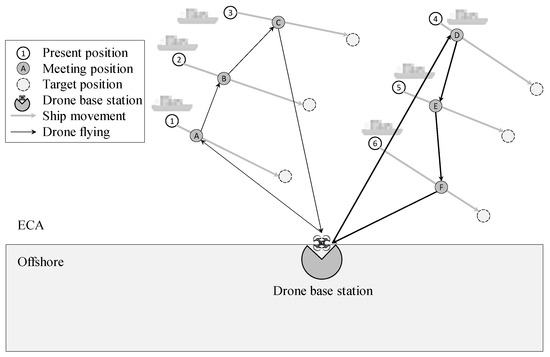
Figure 1. A conceptual diagram of the VRP-based mode.

Many factors are involved in ship pollution emission detection by drones: drone cost, endurance distance, drones, fly distance, detection efficiency, ships, efficiency, fly times, and emergency capability. The number of drones in the fleet will impact these factors. Changing the number of drones in the base station significantly affects the waiting time and detection sequence of ships in ECA. For example, more drones in the fleet may increase detection efficiency while incurring higher drone investment costs.

4. Modeling

Using drones for ship emission detection is an innovative and effective attempt to improve traditional emission detection. To better leverage the utility of drones, we propose a drone routing problem for ship emission detection. Considering the synchronized motion of drones and ships when ships arrive in the ECA, we propose a meeting mode between drones and ships and integrate the motion constraints of drones and ships into the classic VRP, constructing an extended model for this problem.

4.1. Meeting Model between a Drone and a Moving Ship

As studied above, when the drone navigates to the ship’s predetermined “present” position, the ship will have advanced to a new location along its trajectory, as defined by its current and intended positions, as demonstrated in Figure 2. Therefore, it is advantageous to consider the movements of both the drone and ship simultaneously. We calculate the rendezvous point, considering their respective trajectories, and then direct the drone to this estimated position.

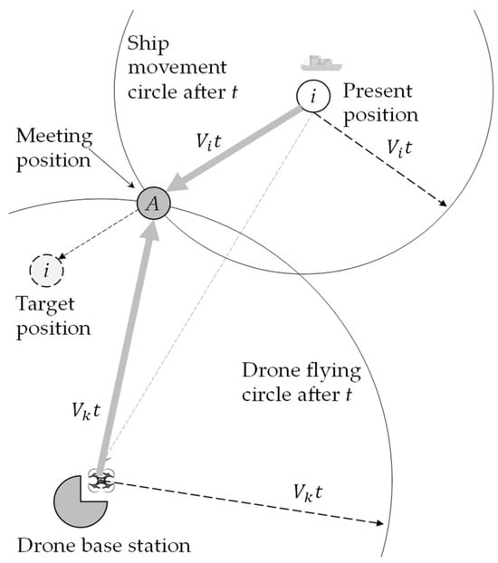
Figure 2. A meeting model for a drone and directional mobile ship.

For a ship $i$ situated at coordinates $\left(X_i,Y_i\right)$, its movement is directed toward a target location $\left(X_i,Y_i\right)$ at a speed $V_i$. Meanwhile, a drone base station k is positioned at $\left({\overline{X}}_k,{\overline{Y}}_k\right)$. If station k deploys a drone at speed ${\overline{V}}_k$ to approach ship $i$, the drone must travel for a duration $t$ to intersect with the moving ship at its target trajectory.

In Figure 2, the point of intersection between the drone and the ship is depicted. The ship moves from point $a(X_i,Y_i)$ to point $b(X_i^t,Y_i^t)$. Two circles can be drawn: one centered at $\left({\overline{X}}_k,{\overline{Y}}_k\right)$ for the drone with a radius of ${\overline{V}}_{k}t$, and another for the ship centered at $\left(X_i,Y_i\right)$ with a radius of $V_{i}t$. The meeting point is where these two circles intersect on the line ab. This intersection is calculated using model (1), where $V_i^X,V_i^Y$ are specified in Equations (2) and (3). The [Mmeet] model can be solved using Equations (4)–(10). A feasible meeting time is then ascertained by Equation (11), disregarding any negative values. The meeting coordinates $\left(x_i,y_i\right)$ are determined by the meeting time t, as calculated in (1).

$$\left\{\begin{array}{c}{x}_i=X_i+t\cdot V_i^X\\ y_i=Y_i+t\cdot V_i^Y\\ \sqrt{{\left(x_i-{\overline{X}}_k\right)}^2+{\left(y_i-{\overline{Y}}_k\right)}^2}=t\cdot {\overline{V}}_k\end{array}\right.$$

(1)

$$V_i^X=V_i\frac{X_i^t-X_i}{\sqrt{{\left(X_i-X_i^t\right)}^2+{\left(Y_i-Y_i^t\right)}^2}}$$

(2)

$$V_i^Y=V_i\frac{Y_i^t-Y_i}{\sqrt{{\left(X_i-X_i^t\right)}^2+{\left(Y_i-Y_i^t\right)}^2}}$$

(3)

$${\left(x_i-{\overline{X}}_k\right)}^2+{\left(y_i-{\overline{Y}}_k\right)}^2=t^2\cdot {\overline{V}}_k^2$$

(4)

$${\left(X_i+t\cdot V_i^X-{\overline{X}}_k\right)}^2+{\left(Y_i+t\cdot V_i^Y-{\overline{Y}}_k\right)}^2=t^2\cdot {\overline{V}}_k^2$$

(5)

$${\left(t\cdot V_i^X+X_i-{\overline{X}}_k\right)}^2+{\left(t\cdot V_i^Y+Y_i-{\overline{Y}}_k\right)}^2=t^2\cdot {\overline{V}}_k^2$$

(6)

$$\left({\left(V_i^X\right)}^2+{\left(V_i^Y\right)}^2-{\overline{V}}_k^2\right)t^2+2\left(V_i^X\left(X_i-{\overline{X}}_k\right)+V_i^Y\left(Y_i-{\overline{Y}}_k\right)\right)t+\left({\left(X_i-{\overline{X}}_k\right)}^2+{\left(Y_i-{\overline{Y}}_k\right)}^2\right)=0$$

(7)

$$a{t}^2+bt+c=0$$

(8)

$$\left\{\begin{array}{c}a={\left(V_i^X\right)}^2+{\left(V_i^Y\right)}^2-{\overline{V}}_k^2\\ b=2\left(V_i^X\left(X_i-{\overline{X}}_k\right)+V_i^Y\left(Y_i-{\overline{Y}}_k\right)\right)\\ c={\left(X_i-{\overline{X}}_k\right)}^2+{\left(Y_i-{\overline{Y}}_k\right)}^2\end{array}\right.$$

(9)

$$t=\frac{-b\pm \sqrt{b^2-4ac}}{2a}$$

(10)

The meeting position $\left(x,y\right)$ and flying time $t^{meet}$ (the valid value in (10)) can be computed for a drone at the base station $k$ and a ship $i$ by the above meeting model, denoted as follows:

$$t^{meet},x_i,y_i\leftarrow f^{\left[\mathrm{m}\mathrm{e}\mathrm{e}\mathrm{t}\right]}\left({\overline{X}}_k,{\overline{Y}}_k,X_i,Y_i,X_i^t,Y_i^t,{\overline{V}}_k,V_i\right).$$

4.2. Baseline VRP Model

The VRP represents a crucial and fundamental problem in combinatorial optimization, gathering extensive attention from numerous researchers [47,48]. In a VRP, the objective is to optimize the routes for a fleet of vehicles to minimize the total travel costs, considering a set of designated customer locations. Using a drone fleet for ship emission detection parallels a VRP scenario, where each drone embarks from a base station and sequentially visits a series of ships, ensuring a single visit per ship. Therefore, we will refer to the VRP models and establish the baseline model.

The baseline model encompasses three distinct sets: a set of ships denoted as $I=\left\{\mathrm{1,2},\cdots \right\}$, indexed by $i$; a set of drones denoted as $K=\left\{\mathrm{1,2},\cdots \right\}$, indexed by $k$; and a combined set of ships and drones denoted as $I^{+}=\left\{\mathrm{1,2},\cdots \right\}$, also indexed by $i$. The variable $C_{ij}$ represents the time taken for a drone to fly from ship $i$ to ship $j$. D denotes the total number of drones available at the station. The binary decision variable $x_{ijk}\in \left\{0,1\right\}$ is set to 1 if drone k is assigned to visit ship $j$ immediately after ship $i$, and 0 otherwise. Similarly, the binary decision variable $y_{ik}\in \left\{\mathrm{0,1}\right\}$, is 1 if drone $k$ is scheduled to visit ship $i$, and 0 otherwise. Additionally, the binary decision variable $u_{ik}$ signifies the sequential order in which ship $i$ is monitored by drone $k$. Utilizing these data and variables, the baseline model is designed to optimize the allocation of ships to drones.

$$\mathrm{m}\mathrm{i}\mathrm{n}{\sum }_{i,j,k}{C}_{ij}{x}_{ijk}$$

(11)

Subject to

$${\sum }_{k\in K}{y}_{ik}=1, \forall i\in N$$

(12)

$${\sum }_{j\in I^{+}}{x}_{ijk}=y_{ik}, \forall i\in N,k\in K$$

(13)

$${\sum }_{j\in I^{+}}{x}_{ijk}={\sum }_{j\in I^{+}}{x}_{jik}, \forall i\in I^{+},k\in K$$

(14)

$$\sum _{i\in I}{y}_{ik}\le D,\forall k\in K$$

(15)

$$u_{ik}+1\le u_{jk}+M\left(1-x_{ijk}\right), \forall i\in I^{+},j\in I,k\in K$$

(16)

$$x_{ijk},y_{ik}\in \left\{\mathrm{0,1}\right\}, \forall i,j\in I^{+},k\in K$$

(17)

$$u_{ik}>0,i\in I^{+},k\in K$$

(18)

In the baseline model, the objective function (11) represents the minimum flight distance of drones; Constraint (12) ensures that each ship must be assigned to an AGV for detection. In Constraint (13), the assignment variable ($y_{ki}$) is presented by the sequencing variable ($x_{kij}$). Namely, ship $i$is detected by drone $k$ if ship $i$ is assigned to drone $k$. Constraint (14) ensures that the in-degree and out-degree of visiting the ship are either one or zero. In Constraint (15), the number of ships detected by each drone is no more than the specific value. Constraint (16) sequences the drone operations, namely, the orders of ships the drones visited. The constraint avoids loops within a route by the order variable of a drone ($k$) visiting two ships ($i,j$). Here, $M=\left|I\right|$. When $x_{ijk}=1$, the constraint is $u_{ik}+1\le u_{jk}$, namely, the orders of visiting the ships $i,j$. Constraint (17) and Constraint (18) constrain the ranges of the variables.

4.3. Extended Model

In the baseline model, $C_{ij}$ represents the traveling time (distance or other costs and metrics) from a position $i$ to another position $j$. In other words, $C_{ij}$ is constant because the positions of $i,j$ are determined and not changed in the model. However, in the ship emission detection scenario, $i,j$ are two moving ships, and the value of $C_{ij}$ depends on the time of the drone visiting the ships. As studied in Section 3, in the ship emission detection scenario, $C_{ij}$ represents the drone’s flying time from a ship $i$ to another ship $j$. A drone visits $j$ just after visiting $i$. A route from the drone base station $k$ can be denoted by $R_k=<k,i_1,i_2,\cdots ,i_n,k>$, where $k$ represents the drone and a virtual depot, and $i_1,i_2,\cdots ,i_n$ represents the visiting sequence of ships. Apparently, $C_{i_a{j}_{a+1}}$ depends on the sequence $<k,i_1,\cdots ,i_a,i_{a+1}]$. Formally, we introduce a function $f^C\left(R_k,i,j\right)$ to present the dependence,

$$C_{ij},\left(x_j,y_j\right)\leftarrow f^C\left(R_k,i,j\right).$$

Here, $R_k=\left\{x_{ijk}=1|\forall i,j\right\}$. Thus,

$$C_{ij},\left(x_j,y_j\right)\leftarrow f^C\left(\left\{x_{ijk}=1|\forall i,j\right\},i,j\right).$$

So, we can update the baseline model and obtain an extended model.

$$\min {\sum }_{i,j,k}{C}_{ij}{x}_{ijk}$$

Subject to

((1)–(18))

$$C_{ij}=f^C\left(\left\{x_{ijk}=1|\forall i,j\right\},i,j\right).$$

(19)

In the extended model, $f^C\left(\cdot \right)$ is a complicated operator that computes the traveling time dependent on the visiting sequence of ships. So, the objective function $C_{ij}{x}_{ijk}$ is nonlinear. Although we formulate the one-station drone VRP based on a linearized one-depot VRP, the extended model is a nonlinear mathematical program. It cannot be solved by one-the-shelf MILP solvers, e.g., Cplex (www.ibm.com/products/ilog-cplex-optimization-studio/cplex-optimizer, accessed on 18 April 2024) and Gurobi (www.gurobi.com, accessed on 18 April 2024).

5. Solution Methods

We develop an SIH-based genetic algorithm to solve this problem. A sequential insert heuristics algorithm is devised to compute the meeting positions and times for a sequence of ships to be visited. The genetic algorithm is used for the iterative solution.

5.1. Sequential Insert Heuristics (SIH)

Based on the meeting model, a sequential insert heuristics algorithm is devised to compute the meeting positions and times for a sequence of ships to be visited. First, initialize the meeting times $t$ and the meeting positions $\left(x,y\right)$. The following information is available: the present and target positions and speed of the ship; the position of the drone base station and the drone’s speed; and a ship sequence to be visited by the drone. Then, by setting the iteration variable $i,$ Set $i=i_1$ to compute the first meeting time $t^{meet}$ and position$(x_i,y_i)$, update $t=t+t^{meet}$, $x=x+\left|x_i\right|,y=y+\left|y_i\right|$. If $i=k$ return $t,x,y$.

The detailed process is shown in Algorithm 1. The algorithm takes a sequence of ships as inputs to generate the times and positions meeting with the drone $k$. In the given six steps, $f^{\left[\mathrm{m}\mathrm{e}\mathrm{e}\mathrm{t}\right]}\left(\cdot \right)$ is invoked to compute the meeting time and position for the ship in the given ship sequence. Then, calculate the meeting time and position with the next ship in this sequence.

Algorithm 1 Sequential insert heuristics (SIH)
Input	$X_i,Y_i,X_i^t,Y_i^t,V_i,\forall i$: the present and target positions and speed of the ship $i$
	${\overline{X}}_k,{\overline{Y}}_k,{\overline{V}}_k$: the position of the drone base station and the drone’s speed
	$R_k= <k,i_1,i_2,\cdots ,i_n,k>$: a ship sequence to be visited by the drone from $k$
Output	$t,x,y$: The meeting times and positions
Steps
Step 1	Initialize outputs
	Set $t=\left[\right],x=\left[\right],y=\left[\right]$.
Step 2	Set the iteration variable $i$
	Set $i=i_1$;
Step 3	Compute the first meeting time and position.
	$t^{meet},x_i,y_i\leftarrow f^{\left[\mathrm{m}\mathrm{e}\mathrm{e}\mathrm{t}\right]}\left({\overline{X}}_k,{\overline{Y}}_k,X_i,Y_i,X_i^t,Y_i^t,{\overline{V}}_k,V_i\right)$.
	Update $t=t+\left[t^{meet}\right],x=x+\left[x_i\right],y=y+\left[y_i\right]$.
Step 4	Termination condition
	If $i=k$ Then, Return $t,x,y$
Step 5	Compute the next meeting time and position
	Set $j=next\left(R_k,i\right)$
	$t^{meet},x_j,y_j\leftarrow f^{\left[\mathrm{m}\mathrm{e}\mathrm{e}\mathrm{t}\right]}\left(x_i,y_i,X_j,Y_j,X_j^t,Y_j^t,{\overline{V}}_k,V_j\right)$.
	Update $t=t+\left[t^{meet}\right],x=x+\left[x_j\right],y=y+\left[y_j\right]$.
Step 6	Update the iteration variable $i$
	$i\leftarrow j$.
	Go to Step 4

Algorithm 1 can be denoted by $f^{\mathrm{S}\mathrm{I}\mathrm{H}}(·)$, as follows.

$$t,x,y\leftarrow f^{\mathrm{S}\mathrm{I}\mathrm{H}}\left(\left[X_i,Y_i,X_i^t,Y_i^t,V_i|\forall i\right],{\overline{X}}_k,{\overline{Y}}_k,{\overline{V}}_k,R_k\right)$$

By $f^{\mathrm{S}\mathrm{I}\mathrm{H}}(·)$, the meeting times $t$ and positions $(x,y)$ between a drone and a sequence of ships can be computed. This is a prerequisite for computing the drone’s and target ship’s total detection time in the following sections. The time complexity of Algorithm 1 is $O\left(n\right)$, where $n$ represents the scale of the number of ships.

5.2. SIH-Based Bi-Stage Solution Algorithm

About the VRP, we have formulated the baseline model to determine the sequence in which a drone visits ships, assuming that the ships are stationary and awaiting detection. This model is then expanded, considering the simultaneous movements of both drones and ships. Subsequently, a two-stage algorithm is developed for this purpose. The first stage involves deriving an initial solution by solving the baseline model, which does not consider the concurrent movements of drones and ships. The second stage employs Sequential Insert Heuristics—Algorithm 1 (SIH)—to translate the ship sequences from the initial solution into actual drone routes, this time factoring in the simultaneous movements of the drones and ships.

The SIH-based bi-stage solution algorithm (Algorithm 2) first solves the VRP to obtain the visit sequence $R$ of drones to ships (Step 1). Then, for each drone visit sequence in turn, the algorithm applies the SIH algorithm—$f^{\mathrm{S}\mathrm{I}\mathrm{H}}\left(\cdot \right)$—to determine the meeting times and positions of each drone visiting the ships (Step 2).

Algorithm 2 Bi-stage algorithm based on One Station VRP and sequential insert decoding ($\mathrm{M}\mathrm{P}+\mathrm{S}\mathrm{I}\mathrm{H}$)
Input	$X_i,Y_i,X_i^t,Y_i^t,V_i,\forall i$: the present and target positions and speed of the ship $i$
	${\overline{X}}_k,{\overline{Y}}_k,{\overline{V}}_k$: the position of the drone base station and the drone’s speed
	$R=\left\{R_k=<k,i_1,i_2,\cdots ,i_n,k>|\forall k\right\}$: a ship sequence to be visited by the drone $k$, obtained by solving [VRP].
Output	$t,x,y$: The meeting times and positions
Steps
Step 1	Solve [VRP].
	$t,R\leftarrow f^{\left[\mathrm{V}\mathrm{R}\mathrm{P}\right]}\left(I,K,C_{ij},Q_k\right)$.
Step 2	For each $R_k$ in $R$
Step 2.1	$t^k,x^k,y^k\leftarrow f^{\mathrm{S}\mathrm{I}\mathrm{H}}\left(\left[X_i,Y_i,X_i^t,Y_i^t,V_i|\forall i\right],{\overline{X}}_k,{\overline{Y}}_k,{\overline{V}}_k,R_k\right)$.
Step 3	Return ${\sum }_{k}last\left(t^k\right)$, $\left[t^k,x^k,y^k|\forall k\right]$

In summary, the first stage (Step 1) solves the baseline model—a mathematical program—to obtain an initial solution, thus denoted by “MP”; in the second stage (Step 2), Algorithm 1 (Sequential Insert Heuristics) is used to convert this initial solution into a solution meeting the constraints in the extended model. So, Algorithm 2 is denoted by $f^{\mathrm{M}\mathrm{P}+\mathrm{S}\mathrm{I}\mathrm{H}}$, as follows,

$$t,x,y\leftarrow f^{\mathrm{M}\mathrm{P}+\mathrm{S}\mathrm{I}\mathrm{H}}\left(\left[X_i,Y_i,X_i^t,Y_i^t,V_i|\forall i\right],\left\{{\overline{X}}_k,{\overline{Y}}_k,{\overline{V}}_k,R_k|\forall k\right\}\right).$$

In Algorithm 2, the second stage can improve the first stage’s solution, while its optimality is constrained by the first stage, which does not consider the simultaneous movements of drones and ships.

5.3. SIH-Based Genetic Algorithm

As a population-based optimization algorithm, the genetic algorithm (GA) is widely used in routing and scheduling problems [49]. During the solving process, the GA first encodes a chromosome string, imitating the biological evolution process, and performs selection, crossover, and mutation to generate chromosomes that are different from and superior to their parents. The new chromosomes are then subjected to the same operations of selection, crossover, and mutation, and this iteration continues until the optimal solution is found in the population. This study encoded ships as a sequence in the chromosome genes, representing their numeric order. The decoding process utilizes a sequential insertion algorithm (Algorithm 1) to translate these sequences into drone detection routes, thereby establishing the meeting positions and times.

The characteristics of the problem are integrated into the GA encoding and decoding techniques. As outlined in Algorithm 2, the solution is encoded in the form of a sequence of ships. The decoder then utilizes this sequence to calculate the specific time and position for the drone’s detection of each ship. The GA devised in this study can be denoted by $f^{\mathrm{G}\mathrm{A}}$ with three sets of algorithmic hyperparameters ($Hparams$) and two problem-related parameters ($Ships,Drones$). Executing $f^{\mathrm{G}\mathrm{A}}$ can produce the meeting time and position for each ship, the assigned drone, and the drones’ visiting sequences of ships.

$$\begin{gathered} \left[R_k,t^k,x^k,y^k|\forall k\right]\leftarrow f^{\mathrm{G}\mathrm{A}}\left(Ships,Drones,Hparams\right) \\ Ships=\left[X_i,Y_i,X_i^t,Y_i^t,V_i|\forall i\right] \\ Drones=\left\{{\overline{X}}_k,{\overline{Y}}_k,{\overline{V}}_k|\forall k\right\} \\ Hparams=\left[P^m,P^x,P^s,P^g,\cdots \right] \end{gathered}$$

5.3.1. The Chromosome Presentation

In this study, the drones used are homogenous, and investment-related decisions predetermine the number. The chromosome consists of a sequence of ship identifiers. For example, a chromosome encoded as integers for 12 ships is as follows: $9\to 8\to 12\to 10\to 1\to 4\to 6\to 5\to 2\to 3\to 11$. The sequence is a permutation of the ships’ identifiers, $\mathrm{1,2},\cdots ,12$. The sequence indicates the priorities of ships to be considered for the assignments of ships to drones and the ships’ emission detection orders. The decoding algorithm (Section 5.3.3) will determine the assignments of ships to drones and each drone’s visiting orders to the ships.

5.3.2. The Decoding Algorithm

The decoding algorithm transforms genetic information generated by GAs into solutions for the given problem. This study uses a real-number encoding scheme. Given a chromosome (a sequence of ships), the ships to be inspected are divided into subsequences for drones using either the drone-by-drone sequence division strategy ($\mathrm{D}\mathrm{r}\mathrm{o}\mathrm{n}\mathrm{e}\mathrm{B}\mathrm{y}\mathrm{D}\mathrm{r}\mathrm{o}\mathrm{n}\mathrm{e}$) or the ship-by-ship sequence division strategy ($\mathrm{S}\mathrm{h}\mathrm{i}\mathrm{p}\mathrm{B}\mathrm{y}\mathrm{S}\mathrm{h}\mathrm{i}\mathrm{p}$). Then, Algorithm 2 (SIH) can decode each subsequence into a feasible solution with determined meeting times and positions for drones and ships.

In summary, the decoding scheme consists of two stages. First, the ships are assigned to drones based on the priorities determined by the chromosome. This stage is entitled “sequence to subsequences” in Section 5.3.3. Second, the ships assigned to a drone constitute a subsequence of ships, which can be used to compute the meeting times and positions by Algorithm 2. In Algorithm 3, the two steps are formulated. The first stage (Step 2 of Algorithm 3) elucidated above is denoted by $divide\left(x,K\right)$. In the second stage (Step 3 of Algorithm 3), the meeting times and positions are computed by $f^{SIH}\left(\cdot \right)$ for each route generated by the first stage.

Algorithm 3 Decoding algorithm
Input	$x$: A chromosome of a sequence of ships
	$divide\left(x,K\right)$: an operator to divide $x$ into $\left|K\right|$ sub-sequences for the stations
	$X_i,Y_i,X_i^t,Y_i^t,V_i,\forall i$: the present and target positions and speed of ship $i$
	${\overline{X}}_k,{\overline{Y}}_k,{\overline{V}}_k$: the position of the drone base station and the drone’s speed
Output	$t$: the total flying time
	$\left[t^k,x^k,y^k|\forall k\right]$: The meeting times and positions of the drones
Steps
Step 1.	Initialize the total flying time.
	$t=0$.
Step 2	Divide the ship sequence into sub-sequences (see Algorithms 4 and 5)
	$R=\left\{R_k|k\in K\right\}\leftarrow divide\left(x,K\right)$.
Step 3	For each $R_k$ in $R$:
	$t^k,x^k,y^k\leftarrow f^{SIH}\left(\left[X_i,Y_i,X_i^t,Y_i^t,V_i|\forall i\right],{\overline{X}}_k,{\overline{Y}}_k,{\overline{V}}_k,R_k\right)$.
	$t=t+t^k$;
Step 4	Return $t,R,\left[t^k,x^k,y^k|\forall k\right]$

5.3.3. Sequence-to-Subsequence Division Strategies

Sequence-to-subsequence division strategies divide a sequence into subsets under specific principles and rules. Section 5.3.3 introduces two methods, namely, $\mathrm{D}\mathrm{r}\mathrm{o}\mathrm{n}\mathrm{e}\mathrm{B}\mathrm{y}\mathrm{D}\mathrm{r}\mathrm{o}\mathrm{n}\mathrm{e}$ and $\mathrm{S}\mathrm{h}\mathrm{i}\mathrm{p}\mathrm{B}\mathrm{y}\mathrm{S}\mathrm{h}\mathrm{i}\mathrm{p}$.

The $\mathrm{D}\mathrm{r}\mathrm{o}\mathrm{n}\mathrm{e}\mathrm{B}\mathrm{y}\mathrm{D}\mathrm{r}\mathrm{o}\mathrm{n}\mathrm{e}$ strategy involves computing the average number of ships that each drone needs to inspect, given a known sequence of drones performing ship pollution inspections and the number of drones available. This average value, denoted by $n$, is used to group about $n$ ships as a batch and assign them to the same drone. Thus, the algorithmic hyperparameters are given as follows: $Hparams=\left[P^m,P^x,P^s,P^g,decode=\mathrm{D}\mathrm{r}\mathrm{o}\mathrm{n}\mathrm{e}\mathrm{B}\mathrm{y}\mathrm{D}\mathrm{r}\mathrm{o}\mathrm{n}\mathrm{e}\right]$. Algorithm 4 gives an implementation of the $\mathrm{D}\mathrm{r}\mathrm{o}\mathrm{n}\mathrm{e}\mathrm{B}\mathrm{y}\mathrm{D}\mathrm{r}\mathrm{o}\mathrm{n}\mathrm{e}$ strategy.

Algorithm 4 Drone-by-drone sequence division strategy ($\mathrm{D}\mathrm{r}\mathrm{o}\mathrm{n}\mathrm{e}\mathrm{B}\mathrm{y}\mathrm{D}\mathrm{r}\mathrm{o}\mathrm{n}\mathrm{e}$)
Input	$x$: A chromosome of a sequence of ships
	$K$: the set of drones
Output	$\left[R_k=<k,i_1,i_2,\cdots ,i_n,k>,\forall k\right]$: the sequences for the drones
Steps
Step 1.	Compute the maximum number of ships visited by a drone.
	$n=⌊\left|x\right|/\left|K\right|⌋$.
Step 2.	Set the sub-sequence for each drone base station.
	$R_k=<k,x_{n\left(k-1\right)+1},\cdots ,x_{nk},k>,\forall k\in K\backslash \left\{\left|K\right|\right\}$.
	$R_k=<k,x_{n\left(k-2\right)+1},\cdots ,x_{\left|x\right|},k>,k=\left|K\right|$.
Step 3.	Return $\left\{R_k|\forall k\right\}$

The $\mathrm{S}\mathrm{h}\mathrm{i}\mathrm{p}\mathrm{B}\mathrm{y}\mathrm{S}\mathrm{h}\mathrm{i}\mathrm{p}$ strategy is an alternative approach to the sequence-to-subsequence division strategies. Under the $\mathrm{S}\mathrm{h}\mathrm{i}\mathrm{p}\mathrm{B}\mathrm{y}\mathrm{S}\mathrm{h}\mathrm{i}\mathrm{p}$ strategy, ships are sequentially assigned to their corresponding drones based on a regular arithmetic progression of the detected ship order. Algorithm 5 implements the $\mathrm{S}\mathrm{h}\mathrm{i}\mathrm{p}\mathrm{B}\mathrm{y}\mathrm{S}\mathrm{h}\mathrm{i}\mathrm{p}$ strategy with $Hparams=\left[P^m,P^x,P^s,P^g,decode=\mathrm{S}\mathrm{h}\mathrm{i}\mathrm{p}\mathrm{B}\mathrm{y}\mathrm{S}\mathrm{h}\mathrm{i}\mathrm{p}\right]$.

Algorithm 5 Ship-by-ship sequence division strategy ($\mathrm{S}\mathrm{h}\mathrm{i}\mathrm{p}\mathrm{B}\mathrm{y}\mathrm{S}\mathrm{h}\mathrm{i}\mathrm{p}$)
Input	$x$: A chromosome of a sequence of ships
	$K$: the drone base stations
Output	$\left[R_k=<k,i_1,i_2,\cdots ,i_n,k>,\forall k\right]$: the sequences for the drones
Steps
Step 1.	Compute the maximum number of ships visited by a drone.
	$n=⌈\left|x\right|/\left|K\right|⌉$.
Step 2.	Set the sub-sequence for each drone base station.
	$R_k=<x_k,\cdots ,x_{nk}|\forall i\in \left\{\mathrm{1,2},\cdots ,n\right\},\exists x_{nk}>,\forall k$.
	$R_k=<k,R_k,k>,\forall k$.
Step 3.	Return $\left\{R_k|\forall k\right\}$

6. Numerical Experiments

This study analyzes the optimization problem of routing a fleet of drones for ship pollution emission detection in ECAs. To validate the effectiveness of the devised models (Section 4) and the GA and its invoking sub-algorithms (Section 5), experimental studies were conducted using Python programming language on a computer with 11th Gen Intel(R) Core (TM) i5-11300H configuration (Intel Corporation, Santa Clara, CA, USA).

6.1. Dataset Generation

In this study, the drone’s speed is fixed at $V_0=25$m per second. Ships within the ECA navigate at speeds uniformly distributed between 10 and 20 knots, roughly equivalent to $V_i~Uniform\left[10,20\right]$ meters per second. Here, $Uniform\left[\mathrm{a},\mathrm{b}\right]$ represents a uniform distribution with the lower and upper limits $a,b$, respectively. The ECA is considered to be located at the Yangtze River estuary, spanning an area of 20 km by 10 km. To abstract from specific real-world locations, this virtual area represents a generic ECA, emphasizing methodological generalizability. The drone’s endurance range varies depending on battery technology, with different types having different capabilities. It is assumed that the drone’s endurance is sufficient for this study, which may influence the setup of ships and the virtual area.

Datasets are generated with the following specifications: The drone base station is positioned at coordinates (0, 0). For each ship, the present and target positions are generated within the $20\times 10$ ($\mathrm{k}\mathrm{m}\times \mathrm{k}\mathrm{m}$) range. The position farther from the drone base station is designated as the present position, while the closest is the target. The pair of present and target positions determine the ship’s direction of movement. The dataset is named in the format $\mathrm{“}\mathrm{K}\mathrm{k}\mathrm{N}\mathrm{n}\mathrm{V}\mathrm{v}\mathrm{X}\mathrm{x}\mathrm{Y}\mathrm{Y}\mathrm{”}$, where K indicates the number of drones at the base station, N the number of ships, V is the drone’s flying speed, X is the horizontal range, and Y the vertical range. For instance, “K2N5V25X20Y10” denotes an ECA spanning $20\times 10 \mathrm{k}{\mathrm{m}}^2$ with two drones at the base station tasked to detect emissions from five ships, and the drones traveling at a speed of $25 \mathrm{m}/\mathrm{s}$.

6.2. Algorithmic Parameter Tuning

The hyperparameters of GA include the number of population iterations ($G$), the population size ($\rho$), the crossover rate ($\alpha$), and the mutation probability ($\beta$). The parameter-tuning experiments used the dataset “K3N30X20Y10V25”. The numerical values of the algorithm parameters are determined through parameter-tuning experiments, where each parameter is adjusted and, others are fixed, and the values that produce the best results are selected.

Figure 3 depicts the optimal values of the GA for various combinations of crossover and mutation probabilities. These two parameters jointly influence the computational efficiency and performance of the GA. The results reveal that a crossover rate of 0.8 and a mutation probability of 0.7 produce the best optimization outcomes. The gray area in Figure 4 shows the parameter combination with the highest objective values.

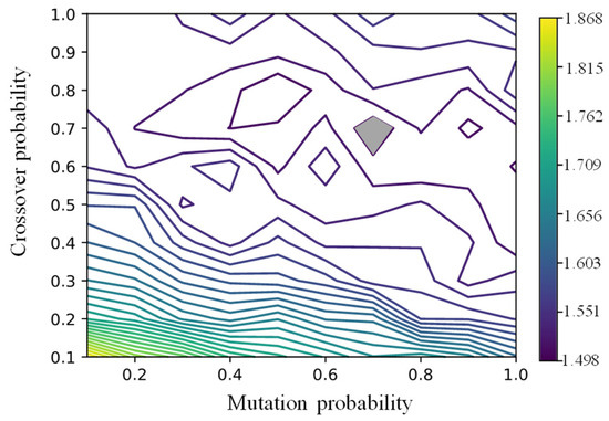
Figure 3. Objectives of various mutation and crossover probabilities.

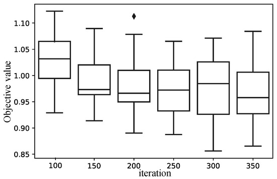
Figure 4. Distributions of objectives for different iterations.

As shown in Figure 4, the mean and distribution of the detection time for multiple drones and ships were investigated for the iterations of the GA. As indicated by the results, we can choose the settings of 250 iterations.

Table 4 shows the impact of population size on the optimal value of the GA. The analysis indicates that the smallest objective function value of the optimal solution is obtained when the population size is 45. As the population size increases, the objective function value remains almost constant while the computation time increases.

Table 4. Average objective values and computing times for various population sizes.

Population Size ($\mathit{G}$)	Best Objective	Computation Time
35	1.354	4.332
40	1.335	4.953
45	1.319	5.515
50	1.330	6.142
55	1.329	6.731
60	1.317	7.329

These results demonstrate the vital role of parameter tuning and iteration adjustment in achieving optimal performance for the GA. Based on the results, the following settings are obtained: $(G,\rho ,\alpha ,\beta )=(250,45,0.7,0.8)$.

6.3. Demonstration of the Models and Algorithms

The dataset “K2N10V10X20Y10” demonstrates the effectiveness of the proposed models and the GAs by using four solutions, as presented in Figure 5. For the demonstration purpose, the present positions of the ships are all set to $\left(0,y_i\right)$ and $y_i$ is distributed from 5 to 10 uniformly. Moreover, the target positions of the ships share the same values of $y_i$. Notably, the devised model and algorithms do not require the ship movement tracks to be paralleled horizontally. So, the ships should move horizontally.

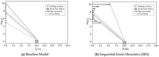
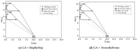
Figure 5. Demonstrations of four solution methods.

In Figure 5a, the ships are presumed to be stationary, not moving, and just waiting for emission detection. Therefore, the meeting positions are still located at $\left(0,y_i\right)$. In Figure 6b, the bi-stage SIH is used. In the first stage, the ships are presumed to be stationary, and the baseline model is used to obtain the assignments of ships to the two drones and the sequence of ships for each drone. So, in Figure 5b, the assignments and sequences of ships to each drone are the same as in Figure 5a. However, the second stage algorithm [SIH] changes the meeting positions and times. In Figure 5b, the movements of ships can be observed. In Figure 5c,d, the $\mathrm{S}\mathrm{h}\mathrm{i}\mathrm{p}\mathrm{B}\mathrm{y}\mathrm{S}\mathrm{h}\mathrm{i}\mathrm{p}$ and $\mathrm{D}\mathrm{r}\mathrm{o}\mathrm{n}\mathrm{e}\mathrm{B}\mathrm{y}\mathrm{D}\mathrm{r}\mathrm{o}\mathrm{n}\mathrm{e}$-based GAs are executed to generate demonstrative results. In these two figures, we can observe no differences. However, when the algorithms are repeated 50 times, the average objectives will incur minor differences, as presented in Table 5. The two decoding strategies will also incur discrepancies in convergence speeds and quality, as shown in Figure 6. The $\mathrm{D}\mathrm{r}\mathrm{o}\mathrm{n}\mathrm{e}\mathrm{B}\mathrm{y}\mathrm{D}\mathrm{r}\mathrm{o}\mathrm{n}\mathrm{e}$ strategy can achieve better solutions while lowering convergency performance more than the $\mathrm{S}\mathrm{h}\mathrm{i}\mathrm{p}\mathrm{B}\mathrm{y}\mathrm{S}\mathrm{h}\mathrm{i}\mathrm{p}\mathrm{s}\mathrm{t}\mathrm{r}\mathrm{a}\mathrm{t}\mathrm{e}\mathrm{g}\mathrm{y}$.

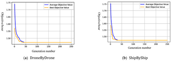
Figure 6. Trace plots of the GAs with $\mathrm{D}\mathrm{r}\mathrm{o}\mathrm{n}\mathrm{e}\mathrm{B}\mathrm{y}\mathrm{D}\mathrm{r}\mathrm{o}\mathrm{n}\mathrm{e}$ and $\mathrm{S}\mathrm{h}\mathrm{i}\mathrm{p}\mathrm{B}\mathrm{y}\mathrm{S}\mathrm{h}\mathrm{i}\mathrm{p}$.

Table 5. The objective values for four different solution approaches.

Solution Method	Objective	Using Meeting Model?
Baseline Model	0.7607	No
Sequential Insert Heuristics (SIH)	0.7515	Yes
GA
$\mathrm{D}\mathrm{r}\mathrm{o}\mathrm{n}\mathrm{e}\mathrm{B}\mathrm{y}\mathrm{D}\mathrm{r}\mathrm{o}\mathrm{n}\mathrm{e}$	0.7429	Yes
$\mathrm{S}\mathrm{h}\mathrm{i}\mathrm{p}\mathrm{B}\mathrm{y}\mathrm{S}\mathrm{h}\mathrm{i}\mathrm{p}$	0.7445	Yes

6.4. Comparisons of the Division Strategies

The impacts of dataset sizes on the division strategies are investigated in Figure 7. The solution methods, $[\mathrm{G}\mathrm{A}+\mathrm{D}\mathrm{r}\mathrm{o}\mathrm{n}\mathrm{e}\mathrm{B}\mathrm{y}\mathrm{D}\mathrm{r}\mathrm{o}\mathrm{n}\mathrm{e}]$ and $[\mathrm{G}\mathrm{A}+\mathrm{S}\mathrm{h}\mathrm{i}\mathrm{p}\mathrm{B}\mathrm{y}\mathrm{S}\mathrm{h}\mathrm{i}\mathrm{p}],$ are executed for the datasets with different numbers of drones ($K$) and ships ($\left|I\right|$), $K=\mathrm{2,3},$ and $\left|I\right|=10,15,\cdots ,50$. With the same number of ships to be detected, the total time for detecting ship pollutants is significantly shorter when using three drones compared to that when using two drones. However, under the same drone quantity condition, adopting the $\mathrm{D}\mathrm{r}\mathrm{o}\mathrm{n}\mathrm{e}\mathrm{B}\mathrm{y}\mathrm{D}\mathrm{r}\mathrm{o}\mathrm{n}\mathrm{e}$ strategy results in shorter drone flight times than when using the ShipByShip strategy. As described in Section 5.3.3, the $\mathrm{D}\mathrm{r}\mathrm{o}\mathrm{n}\mathrm{e}\mathrm{B}\mathrm{y}\mathrm{D}\mathrm{r}\mathrm{o}\mathrm{n}\mathrm{e}$ strategy prioritizes scheduling drone visits to ships based on the number of ships a drone can access, resulting in a sequence of nearby visits. In contrast, the $\mathrm{S}\mathrm{h}\mathrm{i}\mathrm{p}\mathrm{B}\mathrm{y}\mathrm{S}\mathrm{h}\mathrm{i}\mathrm{p}$ strategy assigns each ship to a corresponding drone. Compared with the $\mathrm{D}\mathrm{r}\mathrm{o}\mathrm{n}\mathrm{e}\mathrm{B}\mathrm{y}\mathrm{D}\mathrm{r}\mathrm{o}\mathrm{n}\mathrm{e}$ strategy, the ShipByShip strategy may require the detection of ships that are further apart from each other, and as ships and drones move synchronously, the flight time during the drone’s visit to a ship increases when the ship being visited is farther away.

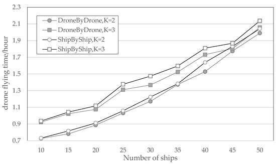
Figure 7. Comparisons of the $\mathrm{D}\mathrm{r}\mathrm{o}\mathrm{n}\mathrm{e}\mathrm{B}\mathrm{y}\mathrm{D}\mathrm{r}\mathrm{o}\mathrm{n}\mathrm{e}$ strategy and $\mathrm{S}\mathrm{h}\mathrm{i}\mathrm{p}\mathrm{B}\mathrm{y}\mathrm{S}\mathrm{h}\mathrm{i}\mathrm{p}$ strategy.

6.5. Sensitivities of Ships and Drones’ Speeds

The speeds of both drones $V_0$ and ships $V_i$ are contingent upon technological advancements and investments. Increasing the speeds of ships and drones results in higher energy expenditures and augmented emissions. Additionally, technological limitations can restrict the maximum achievable speeds of drones. Accelerating drone speeds might necessitate innovation and further investment. In the subsequent analysis, we explore how variations in the speeds of drones and ships affect the total operational time.

Table 6 presents the sensitivity of the ships’ speeds ($V_i$) by varying them −5% and 5% and the sensitivity of the drones’ speeds ($V_i$) by varying them −5% and 5%. From the information in Table 6, we can see that the increase or decrease in the shipping speed does not show an apparent correlation regularity on the effect of the objective function, while the rise in the drone flight speed can effectively decrease the value of the objective function; the decline in the drone flight speed will make the value of the objective function grow larger. As presented in Figure 7, improving the flight speed of drones is probably more effective for optimizing the detection time of multi-drone ship pollution emissions.

Table 6. Sensitivity of the ships’ speeds ($V_i$) and drones’ speeds ($V_k$).

			${\mathit{V}}_{\mathit{i}}$			${\mathit{V}}_{\mathit{k}}$
Stations	Ships	(100 − 5)%	100%/h	(100 + 5)%	(100 − 5)%	100%/h	(100 + 5)%
2	10	−0.04	0.76	−0.20	4.70	0.76	−2.86
2	15	−0.07	0.83	−3.48	3.82	0.83	−7.11
2	20	−2.80	0.93	−2.14	2.75	0.93	−3.66
2	25	1.97	1.04	1.54	5.58	1.04	2.44
2	30	−1.24	1.22	−8.40	4.32	1.22	−15.50
2	35	4.69	1.28	6.75	9.48	1.28	−10.90
2	40	−1.14	1.51	−2.24	2.98	1.51	−11.74
2	45	5.01	1.63	−2.54	6.58	1.63	3.31
2	50	−3.27	2.00	−2.54	−2.42	2.00	−6.83
3	10	−0.13	0.95	0.24	5.24	0.95	−5.04
3	15	2.87	1.08	4.27	6.63	1.08	−5.29
3	20	0.04	1.12	1.25	11.79	1.12	0.69
3	25	2.32	1.32	5.72	10.56	1.32	−3.78
3	30	−2.78	1.49	1.73	1.86	1.49	−7.58
3	35	−1.31	1.68	−2.77	−2.18	1.68	−14.29
3	40	2.48	1.75	4.64	7.15	1.75	−10.20
3	45	−2.31	2.02	−9.46	−0.62	2.02	−7.87
3	50	2.79	2.25	−6.38	−0.60	2.25	−8.05

As presented in Figure 8, it is evident that the drones’ speed significantly impacts the flight time required to complete ship-pollution-monitoring tasks. The effect of drone speed on flight time was analyzed for two and three drones, with task numbers N ranging from 10 to 50. The results show that increasing drone speed leads to a noticeable decrease in flight time, whereas decreasing drone speed leads to a significant increase in flight time. Figure 9 reveals that under the same conditions of drone quantity, $V_i\left(1-5\mathrm{\%}\right)$, $V_i$, and $V_i\left(1+5\mathrm{\%}\right)$ almost overlap. This indicates that changes in ship speed do not significantly impact the flight time required for drones to complete ship-pollution-monitoring tasks.

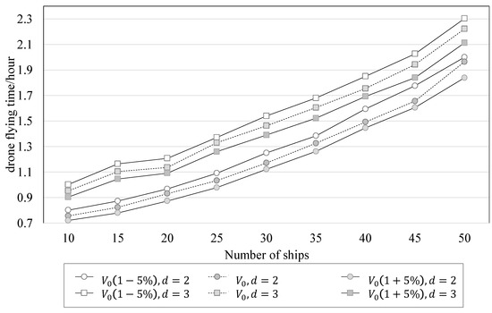
Figure 8. Sensitivity analysis of drones’ speed.

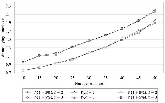
Figure 9. A diagram of ships’ speed sensitivity analysis.

6.6. Discussions and Managerial Implications

Using drones for ship pollution monitoring in ECA is an innovative way to monitor ship emissions at sea, and it offers higher monitoring efficiency than traditional monitoring methods. The establishment of ECA has set clear targets and regulations for ship emission reduction in specific areas, but practical implementation of these policies requires efficient regulatory methods and execution capabilities. To achieve effective regulation, it is necessary to optimize the deployment of drones for ship monitoring tasks. In this study, we formulate the problem of efficient and reasonable ship emission detection as a multi-drone routing optimization problem.

We draw the following conclusions as managerial implications based on the experimental results.

(1)

The optimization of drone flight routing for ship emission detection is a dynamic problem involving the simultaneous movement of drones and ships. The proposed meeting model can appropriately characterize the dynamic problem. The model is an extension and theoretical increment to the static VRP problem. In addition, the meeting model complements the study of operations research theory on dynamic problems. In practice, compared to single drones, multi-drone and ship meeting models based on the VRP model can overcome the difficulties of low detection efficiency and long flight distances. Experiments have verified their advantages in applications.

(2)

Regarding detection efficiency, the DroneByDrone strategy has an advantage over the ShipByShip strategy in terms of performance. The reason is that with drones traveling at much higher speeds than ships, the DroneByDrone strategy prioritizes the drone detection sequence, thereby reducing the detection time. In addition, in the meeting problem, fast-moving objects should be used as the entry point for algorithm design. Therefore, the DroneByDrone strategy should be prioritized to handle the drone routing problem. However, the meeting model is nonlinear, and it is not easy to find an exact solution. Thus, linearization methods need further research to save costs.

(3)

Our research focuses on the scheduling problem of drones at the operational level, with the understanding that coordination mechanisms and information systems are vital determinants of operational performance. First, an effective drone scheduling system must dynamically track the positions of ships using data acquired from AIS receivers. Second, drone base stations must exchange scheduling information and integrate their schedules into a centralized, top-level scheduling system. This integration facilitates the global deployment of drones. Third, local ECA authorities should collaborate in sharing the schedules for ship emission detection and the resulting data, ensuring comprehensive monitoring and management.

7. Conclusions

The adverse effects of ship emissions on the ecological environment and human health in coastal areas have prompted a need for innovative ship emission detection methods. In this regard, we investigated the optimization problem of drone routing in ship emission detection. Firstly, effective detection methods are necessary for the ECA to achieve good ship emission monitoring and control effects, thereby reducing the impact of ship emissions on people’s health in the coastal areas. Traditional detection methods suffer from low efficiency and cumbersome procedures. Using drones for ship emission detection is an innovative and effective attempt to improve traditional emission detection. To better leverage the utility of drones, we propose a multi-drone routing optimization problem for ship emission detection. Secondly, considering the synchronized motion of drones and ships when ships arrive in the ECA, we propose a meeting mode between drones and ships and integrate the motion constraints of drones and ships into the classic VRP, constructing an extended model for this problem. Thirdly, we develop an SIH-based genetic algorithm to solve this problem. The sequence insertion algorithm determines the meeting time and location of drones and ships, and the genetic algorithm is used for the iterative solution. Finally, taking the Yangtze River Delta ECA as an example, we develop a dataset generation method and conduct experiments to demonstrate and study the proposed model, algorithm, and sensitivity analysis.

Our study proposes an innovative and practical approach to ship emission detection using drones and develops a multi-drone routing optimization model and an SIH-based genetic algorithm for solving it. The experimental results demonstrate the effectiveness and feasibility of the proposed method, which can be applied to other ECA or environmental monitoring tasks. The baseline Model (Section 4.2) can obtain routes while not considering dynamic simultaneous movements of ships and drones; it, coupled with SIH, can constitute the bi-stage solution algorithm. Further, a GA can use SIH as a decoding algorithm with two strategies to allocate ships to drone routes, DroneByDrone, and ShipByShip. The bi-stage and the GAs (with DroneByDrone or ShipByShip) can solve the drone routing problem, while the bi-stage is not competitive compared with the latter two methods.

In future research, this study can be expanded in several ways:

(1)

The base station for drone flights is currently fixed and singular. Future research could explore the possibility of having multiple base stations in an ECA and optimizing the selection of base station locations in conjunction with drone detection routing to minimize drone detection routing and achieve better management and economic value. Additionally, the genetic algorithm based on sequence insertion used in this study is effective but cannot guarantee optimality. Future research could develop more efficient algorithms to solve this problem.

(2)

Implementing machine learning and artificial intelligence techniques could be explored to improve the accuracy and efficiency of the drone detection system. This could involve training models to identify patterns in drone flight routing and predict potential breaches of the ECA. Additionally, the use of advanced sensors and imaging technologies could be investigated to enhance the system’s detection capabilities.

(3)

The potential for integrating the drone detection system with other security systems could be explored. For example, the system could be integrated with perimeter intrusion detection or video surveillance systems to provide a comprehensive security solution. This would require careful consideration of data integration and sharing protocols to ensure seamless integration and optimal performance.

References

- Liu, J.; Law, A.W.-K.; Duru, O. Abatement of atmospheric pollutant emissions with autonomous shipping in maritime transportation using Bayesian probabilistic forecasting. Atmos. Environ. 2021, 261, 118593. [Google Scholar] [CrossRef]
- Tokuslu, A. Estimating greenhouse gas emissions from ships on four ports of Georgia from 2010 to 2018. Environ. Monit. Assess. 2021, 193, 385. [Google Scholar] [CrossRef] [PubMed]
- Wan, Z.; Zhang, Q.; Xu, Z.; Chen, J.; Wang, Q. Impact of emission control areas on atmospheric pollutant emissions from major ocean-going ships entering the Shanghai Port, China. Mar. Pollut. Bull. 2019, 142, 525–532. [Google Scholar] [CrossRef] [PubMed]
- Wan, Z.; Zhou, X.; Zhang, Q.; Chen, J. Influence of sulfur emission control areas on particulate matter emission: A difference-in-differences analysis. Mar. Policy 2021, 130, 104584. [Google Scholar] [CrossRef]
- Zhang, Q.; Liu, H.; Wan, Z. Evaluation on the effectiveness of ship emission control area policy: Heterogeneity detection with the regression discontinuity method. Environ. Impact Assess. Rev. 2022, 94, 106747. [Google Scholar] [CrossRef]
- Jiang, B.; Wang, X.; Xue, H.; Li, J.; Gong, Y. An evolutionary game model analysis on emission control areas in China. Mar. Policy 2020, 118, 104010. [Google Scholar] [CrossRef]
- Sun, Y.; Yang, L.; Zheng, J. Emission control areas: More or fewer? Transp. Res. Part D Transp. Environ. 2020, 84, 102349. [Google Scholar] [CrossRef]
- Chang, Y.-T.; Park, H.; Lee, S.; Kim, E. Have Emission Control Areas (ECAs) harmed port efficiency in Europe? Transp. Res. Part D Transp. Environ. 2018, 58, 39–53. [Google Scholar] [CrossRef]
- Tian, X.; Yan, R.; Qi, J.; Zhuge, D.; Wang, H. A Bi-Level Programming Model for China’s Marine Domestic Emission Control Area Design. Sustainability 2022, 14, 3562. [Google Scholar] [CrossRef]
- Chang, Y.-T.; Roh, Y.; Park, H. Assessing noxious gases of vessel operations in a potential Emission Control Area. Transp. Res. Part D Transp. Environ. 2014, 28, 91–97. [Google Scholar] [CrossRef]
- Okada, A. Benefit, cost, and size of an emission control area: A simulation approach for spatial relationships. Marit. Policy Manag. 2019, 46, 565–584. [Google Scholar] [CrossRef]
- Dong, G.; Tae-Woo Lee, P. Environmental effects of emission control areas and reduced speed zones on container ship operation. J. Clean. Prod. 2020, 274, 122582. [Google Scholar] [CrossRef]
- Fan, L.; Yu, Y.; Yin, J. Impact of Sulphur Emission Control Areas on port state control’s inspection outcome. Marit. Policy Manag. 2022, 50, 1–16. [Google Scholar] [CrossRef]
- Ma, D.; Ma, W.; Jin, S.; Ma, X. Method for simultaneously optimizing ship route and speed with emission control areas. Ocean Eng. 2020, 202, 107170. [Google Scholar] [CrossRef]
- Chen, L.; Yip, T.L.; Mou, J. Provision of Emission Control Area and the impact on shipping route choice and ship emissions. Transp. Res. Part D Transp. Environ. 2018, 58, 280–291. [Google Scholar] [CrossRef]
- Ma, W.; Hao, S.; Ma, D.; Wang, D.; Jin, S.; Qu, F. Scheduling decision model of liner shipping considering emission control areas regulations. Appl. Ocean Res. 2021, 106, 102416. [Google Scholar] [CrossRef]
- Li, L.; Gao, S.; Yang, W.; Xiong, X. Ship’s response strategy to emission control areas: From the perspective of sailing pattern optimization and evasion strategy selection. Transp. Res. Part E Logist. Transp. Rev. 2020, 133, 101835. [Google Scholar] [CrossRef]
- Šilas, G.; Rapalis, P.; Lebedevas, S. Particulate Matter (PM1, 2.5, 10) Concentration Prediction in Ship Exhaust Gas Plume through an Artificial Neural Network. J. Mar. Sci. Eng. 2023, 11, 150. [Google Scholar] [CrossRef]
- Zhang, Z.; Zheng, W.; Cao, K.; Li, Y.; Xie, M. Simulation Analysis on the Optimal Imaging Detection Wavelength of SO2 Concentration in Ship Exhaust. Atmosphere 2020, 11, 1119. [Google Scholar] [CrossRef]
- Bui, K.Q.; Perera, L.P. Advanced data analytics for ship performance monitoring under localized operational conditions. Ocean Eng. 2021, 235, 109392. [Google Scholar] [CrossRef]
- Guo, J.; Guo, L. Research on SOX online detection system of marine diesel engine based on LabVIEW. J. Mar. Sci. Technol. 2022, 27, 1179–1191. [Google Scholar] [CrossRef]
- Rapalis, P.; Šilas, G.; Žaglinskis, J. Ship Air Pollution Estimation by AIS Data: Case Port of Klaipeda. J. Mar. Sci. Eng. 2022, 10, 1950. [Google Scholar] [CrossRef]
- Zhou, C.; Huang, H.; Liu, Z.; Ding, Y.; Xiao, J.; Shu, Y. Identification and analysis of ship carbon emission hotspots based on data field theory: A case study in Wuhan Port. Ocean Coast. Manag. 2023, 235, 106479. [Google Scholar] [CrossRef]
- Georgoulias, A.K.; Boersma, K.F.; van Vliet, J.; Zhang, X.; Zanis, P.; de Laat, J. Detection of NO2 pollution plumes from individual ships with the TROPOMI/S5P satellite sensor. Environ. Res. Lett. 2020, 15, 124037. [Google Scholar] [CrossRef]
- Czermański, E.; Cirella, G.T.; Oniszczuk-Jastrząbek, A.; Pawłowska, B.; Notteboom, T. An Energy Consumption Approach to Estimate Air Emission Reductions in Container Shipping. Energies 2021, 14, 278. [Google Scholar] [CrossRef]
- Zhang, Z.; Zheng, W.; Cao, K.; Li, Y.; Xie, M. An improved method for optimizing detection bands of marine exhaust SO2 concentration in ultraviolet dual-band measurements based on signal-to-noise ratio. Atmos. Pollut. Res. 2022, 13, 101479. [Google Scholar] [CrossRef]
- Beirle, S. Estimate of nitrogen oxide emissions from shipping by satellite remote sensing. Geophys. Res. Lett. 2004, 31, L18102. [Google Scholar] [CrossRef]
- Peng, X.; Huang, L.; Wu, L.; Zhou, C.; Wen, Y.; Chen, H.; Xiao, C. Remote detection sulfur content in fuel oil used by ships in emission control areas: A case study of the Yantian model in Shenzhen. Ocean Eng. 2021, 237, 109652. [Google Scholar] [CrossRef]
- Kuzniar, M.; Pawlak, M.; Orkisz, M. Comparison of Pollutants Emission for Hybrid Aircraft with Traditional and Multi-Propeller Distributed Propulsion. Sustainability 2022, 14, 15076. [Google Scholar] [CrossRef]
- Anand, A.; Wei, P.; Gali, N.K.; Sun, L.; Yang, F.H.; Westerdahl, D.; Zhang, Q.; Deng, Z.Q.; Wang, Y.; Liu, D.G.; et al. Protocol development for real-time ship fuel sulfur content determination using drone based plume sniffing microsensor system. Sci. Total Environ. 2020, 744, 140885. [Google Scholar] [CrossRef]
- Paradiso, R.; Roberti, R.; Laganá, D.; Dullaert, W. An Exact Solution Framework for Multitrip Vehicle-Routing Problems with Time Windows. Oper. Res. 2020, 68, 180–198. [Google Scholar] [CrossRef]
- Dell’Amico, M.; Montemanni, R.; Novellani, S. Matheuristic algorithms for the parallel drone scheduling traveling salesman problem. Ann. Oper. Res. 2020, 289, 211–226. [Google Scholar] [CrossRef]
- Salama, M.R.; Srinivas, S. Collaborative truck multi-drone routing and scheduling problem: Package delivery with flexible launch and recovery sites. Transp. Res. Part E-Logist. Transp. Rev. 2022, 164, 102788. [Google Scholar] [CrossRef]
- Xu, J.; Liu, C.; Shao, J.; Xue, Y.; Li, Y. Collaborative orchard pesticide spraying routing problem with multi-vehicles supported multi-UAVs. J. Clean. Prod. 2024, 458, 142429. [Google Scholar] [CrossRef]
- Roberti, R.; Ruthmair, M. Exact Methods for the Traveling Salesman Problem with Drone. Transp. Sci. 2021, 55, 315–335. [Google Scholar] [CrossRef]
- Gentili, M.; Mirchandani, P.B.; Agnetis, A.; Ghelichi, Z. Locating platforms and scheduling a fleet of drones for emergency delivery of perishable items. Comput. Ind. Eng. 2022, 168, 108057. [Google Scholar] [CrossRef]
- Mukhamediev, R.I.; Yakunin, K.; Aubakirov, M.; Assanov, I.; Kuchin, Y.; Symagulov, A.; Levashenko, V.; Zaitseva, E.; Sokolov, D.; Amirgaliyev, Y. Coverage Path Planning Optimization of Heterogeneous UAVs Group for Precision Agriculture. IEEE Access 2023, 11, 5789–5803. [Google Scholar] [CrossRef]
- Wang, Y.; Wang, Z.; Hu, X.; Xue, G.; Guan, X. Truck-drone hybrid routing problem with time-dependent road travel time. Transp. Res. Part C-Emerg. Technol. 2022, 144, 103901. [Google Scholar] [CrossRef]
- Schermer, D.; Moeini, M.; Wendt, O. A hybrid VNS/Tabu search algorithm for solving the vehicle routing problem with drones and en route operations. Comput. Oper. Res. 2019, 109, 134–158. [Google Scholar] [CrossRef]
- Poikonen, S.; Golden, B. Multi-visit drone routing problem. Comput. Oper. Res. 2020, 113, 104802. [Google Scholar] [CrossRef]
- Amorosi, L.; Puerto, J.; Valverde, C. Coordinating drones with mothership vehicles: The mothership and drone routing problem with graphs. Comput. Oper. Res. 2021, 136, 105445. [Google Scholar] [CrossRef]
- Tamke, F.; Buscher, U. A branch-and-cut algorithm for the vehicle routing problem with drones. Transp. Res. Part B-Methodol. 2021, 144, 174–203. [Google Scholar] [CrossRef]
- Huang, S.-H.; Huang, Y.-H.; Blazquez, C.A.; Chen, C.-Y. Solving the vehicle routing problem with drone for delivery services using an ant colony optimization algorithm. Adv. Eng. Inform. 2022, 51, 101536. [Google Scholar] [CrossRef]
- Jung, H.; Kim, J. Drone scheduling model for delivering small parcels to remote islands considering wind direction and speed. Comput. Ind. Eng. 2022, 163, 107784. [Google Scholar] [CrossRef]
- Miguel Leon-Blanco, J.; Gonzalez, P.L.; Andrade-Pineda, J.L.; Canca, D.; Calle, M. A multi-agent approach to the truck multi-drone routing problem. Expert Syst. Appl. 2022, 195, 116604. [Google Scholar] [CrossRef]
- Zeng, F.; Chen, Z.; Clarke, J.-P.; Goldsman, D. Nested vehicle routing problem: Optimizing drone-truck surveillance operations. Transp. Res. Part C-Emerg. Technol. 2022, 139, 103645. [Google Scholar] [CrossRef]
- Braekers, K.; Ramaekers, K.; Van Nieuwenhuyse, I. The vehicle routing problem: State of the art classification and review. Comput. Ind. Eng. 2016, 99, 300–313. [Google Scholar] [CrossRef]
- Pillac, V.; Gendreau, M.; Gueret, C.; Medaglia, A.L. A review of dynamic vehicle routing problems. Eur. J. Oper. Res. 2013, 225, 1–11. [Google Scholar] [CrossRef]
- Potvin, J.Y. State-of-the Art Review Evolutionary Algorithms for Vehicle Routing. Inf. J. Comput. 2009, 21, 518–548. [Google Scholar] [CrossRef]
Disclaimer/Publisher’s Note: The statements, opinions and data contained in all publications are solely those of the individual author(s) and contributor(s) and not of MDPI and/or the editor(s). MDPI and/or the editor(s) disclaim responsibility for any injury to people or property resulting from any ideas, methods, instructions or products referred to in the content. |
© 2024 by the authors. Licensee MDPI, Basel, Switzerland. This article is an open access article distributed under the terms and conditions of the Creative Commons Attribution (CC BY) license (https://creativecommons.org/licenses/by/4.0/).