1. Introduction
With the continuous evolution of maritime logistics, the integration of intelligence and technology has gained significant attention. Within this domain, intelligent navigation plays a pivotal role, and vessel navigation situational awareness has emerged as a critical element. In recent years, inland waterway transport has experienced rapid development, resulting in the accumulation of a substantial repository of foundational data resources. These resources encompass various aspects, such as channel surveying, lock scheduling, operational vessel information, AIS data, radar images, and more. However, the intricate nature of inland waterways, characterized by complex shorelines, winding channels, high vessel traffic densities, and frequent vessel encounters, poses substantial constraints on situational awareness, especially on perception data association and fusion. In addition, inland intelligent ship navigation systems primarily focus on intelligent ships as the central element [
1]. The key to intelligent ships lies in the association of multi-source data in navigation situational awareness [
2]. Conducting research on the association of perception data in inland vessel navigation is essential for enhancing intelligent situational awareness. Therefore, this research endeavor contributes to the advancement of industrial technology in inland intelligent vessels.
In maritime navigation situational awareness, perception data primarily originate from various sensors, such as radar, AIS, remote sensing satellites, and BeiDou [
3], which is a global navigation satellite system (GNSS) similar to other GNSS systems like GPS (Global Positioning System) and GLONASS (Global Navigation Satellite System). BeiDou provides precise positioning, navigation, and timing services to users worldwide and especially prevails in passenger ships and fishing ships in China. Radar is one of the primary sensor technologies for improving navigation safety. While small plastic or wooden boats without AIS systems may not have as strong a radar signature as metal-hulled vessels, radar is still capable of detecting plastic or wooden vessels, such as fishing boats, within a certain range, typically up to 3 km. Multi-source data invariably contain a variety of noise and interruptions in trajectory continuity that arise from signal disruptions, introducing uncertainties in navigation situational awareness. Therefore, achieving more precise target association and perception is of the utmost importance when dealing with multi-source trajectory data. Singer introduced the nearest-neighbor method, which employs a distance gating approach to eliminate spurious targets. This algorithm measures the similarity between different trajectories, enabling the determination of trajectory associations [
4]. Bar- Shalom et al. proposed a probabilistic data association approach for trajectory association in single-target scenarios [
5]. These methods are characterized by their simplicity and low computational loads. However, their performance tends to degrade in areas with complex traffic patterns and high levels of noise [
6].
In addressing the intricate and multi-track fusion scenarios present in maritime surveillance data, Ming et al. introduced a weighted trajectory fusion algorithm leveraging local information entropy for the integration of AIS and X-band radar data [
7]. And, based on fuzzy theory, Liu proposed a trajectory association method for AIS and surface wave radar (SWR) based on a fuzzy dual-threshold approach. This method utilizes fuzzy membership to quantify the degree of association between trajectories and employs dual-threshold detection to determine associated trajectory pairs [
8]. In addition to AIS and SWR data, synthetic aperture radar (SAR) data and satellite images are employed to facilitate trajectory association for the objective of ship traffic monitoring in open seas [
9,
10]. With the advancement of deep learning, relevant techniques have also been applied to ship trajectory association. Jin et al. integrated track and scene features to estimate the probability of track association by deep learning [
11]. Simulation results reveal the method’s superior scene adaptability and association accuracy compared to traditional approaches. And Yang et al. developed a multi-target association algorithm for AIS–radar tracks using a graph matching-based deep neural network [
12]. The above-mentioned method primarily relies on shore-based equipment and is commonly applied in vessel perception data association research in coastal areas and validated through simulation to assess its effectiveness in real-world scenarios. However, the navigational environment in inland waterways is significantly distinct, exhibiting intricate shorelines, convoluted channels, and diverse inland electronic interference factors. Consequently, the practical applicability of these methods in such environments necessitates further validation.
In inland waterways, closed-circuit television (CCTV) is prevalent in management to enhance traffic situational awareness and monitor abnormal vessel behavior due to its remote and real-time capabilities [
13]. Guo et al. incorporated a dynamic time warping algorithm that calculates the similarity of AIS- and CCTV-based vessel trajectories to improve vessel traffic surveillance in inland waterways [
14]. Huang et al. established a ship information fusion model based on CCTV images and AIS data, specifically focusing on the tracking of ships [
15]. By employing the YOLOv3 algorithm, Gan et al. presented a vision-based data fusion approach for enhancing environmental awareness in ship navigation [
16]. In addition to the fusion of CCTV and AIS data, it is also employed for radar data integration to facilitate ship target detection. Liu proposed a method of multi-scale matching vessel recognition (MSM-VR) by fusing CCTV and marine radar to ensure navigation safety [
17]. CCTV surveillance systems are susceptible to adverse weather conditions, such as rain, fog, and strong winds. These conditions can result in blurred or obstructed visibility, thereby potentially compromising their detection performance. However, advanced CCTV systems with multi-spectral or thermal imaging technology often outperform human vision, particularly in challenging visibility conditions and nighttime operations. Additionally, their capabilities for accurately measuring distances and sizes are limited, making the recognition of distant or smaller vessels challenging. As a result, the identification of remote or compact vessels may prove to be a challenging task.
Maritime ship track association methods are mainly based on statistical methods and fuzzy mathematics, including the nearest-neighbor (NN) method, fuzzy double thresholds, fuzzy comprehensive functions, etc. Nearest-neighbor data association is a relatively simple method and mainly suitable for situations in which there is little noise and scenarios with a small number of targets [
18]. Due to factors such as random noise and the inconsistent detection ranges of different sensors, there is ambiguity in the similarity between their tracks, and fuzzy mathematics has been applied to judge track associations [
19,
20]. However, existing vessel navigation perception techniques, primarily designed for coastal and open-water areas, require validation and refinement for inland waterway applications. Furthermore, inland waterways primarily emphasize the fusion of video images and AIS data, which have the capability to detect objects not discernible by radar or lacking AIS data, while research into AIS and radar trajectory association methods for shipborne perception systems is lacking. Moreover, AIS and radar systems are usually mandatory equipment for vessels according to maritime regulations, so it is essential to enhance the accuracy and reliability of vessel position and motion information to compensate for the limitations of each system and provide more accurate vessel positions, aiding in real-time adjustment of course and speed to maintain safe distances at sea. Therefore, this study focuses on vessel association of shipborne data in inland waterway vessels by leveraging trajectory features. By employing machine learning and harnessing trajectory information, this research endeavors to enhance the precision and efficacy of vessel situational awareness, thereby contributing to the safety and intelligence of inland waterway navigation. There are two specific contributions of this paper:
We propose a novel classifier approach that incorporates trajectory characteristics to solve data association issues in inland waterways.
We propose a dataset construction method to build positive and negative sample datasets for data association using labeled shipborne perception data.
The rest of the paper is organized as follows: the methodology is introduced in
Section 2, the computation of trajectory features is detailed in
Section 3, the dataset construction is described in
Section 4, and the experiments conducted for the method analysis and validation are described in
Section 5.
2. Methods
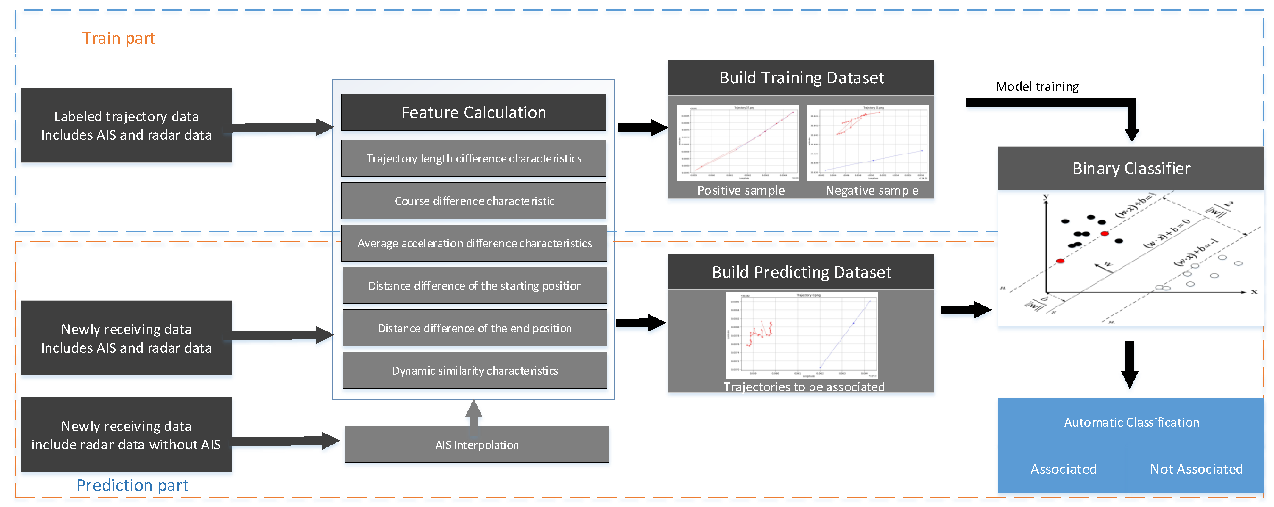
This paper employs a binary classification method based on trajectory features to achieve ship target association from AIS and radar data in intelligent navigation perception systems, as illustrated in
Figure 1. The approach encompasses trajectory feature calculation, positive and negative sample dataset construction, and support vector machine (SVM) model development. Initially, trajectory feature calculation is performed on the training dataset. Subsequently, a training set is constructed with radar and AIS trajectory features extracted from the targets, encompassing both positive and negative samples. Then, trajectory feature calculation is performed on the prediction dataset to establish the features of the trajectories that require association. Finally, an SVM model is built using the constructed dataset for training and predicting newly received AIS and radar data. In cases where AIS data are missing, interpolated AIS data along with radar data are utilized to make predictions.
2.1. SVM Model
Ship radar and AIS are two prevalent ship monitoring technologies that capture ship position and movement data via radio waves and signals. However, the integration of data from these two distinct sources poses a noteworthy challenge stemming from their unique characteristics and inherent incompleteness. The Support Vector Machine (SVM), a supervised learning algorithm, was originally proposed by Vladimir Vapnik [
21]. Since its inception, it has undergone continuous development and refinement, emerging as a prominent algorithm in machine learning with wide-ranging applications in pattern recognition, classification, and regression tasks. This section will delve into the fundamental principles of the SVM and explore its utilization in the association and classification of ship radar and AIS track data.
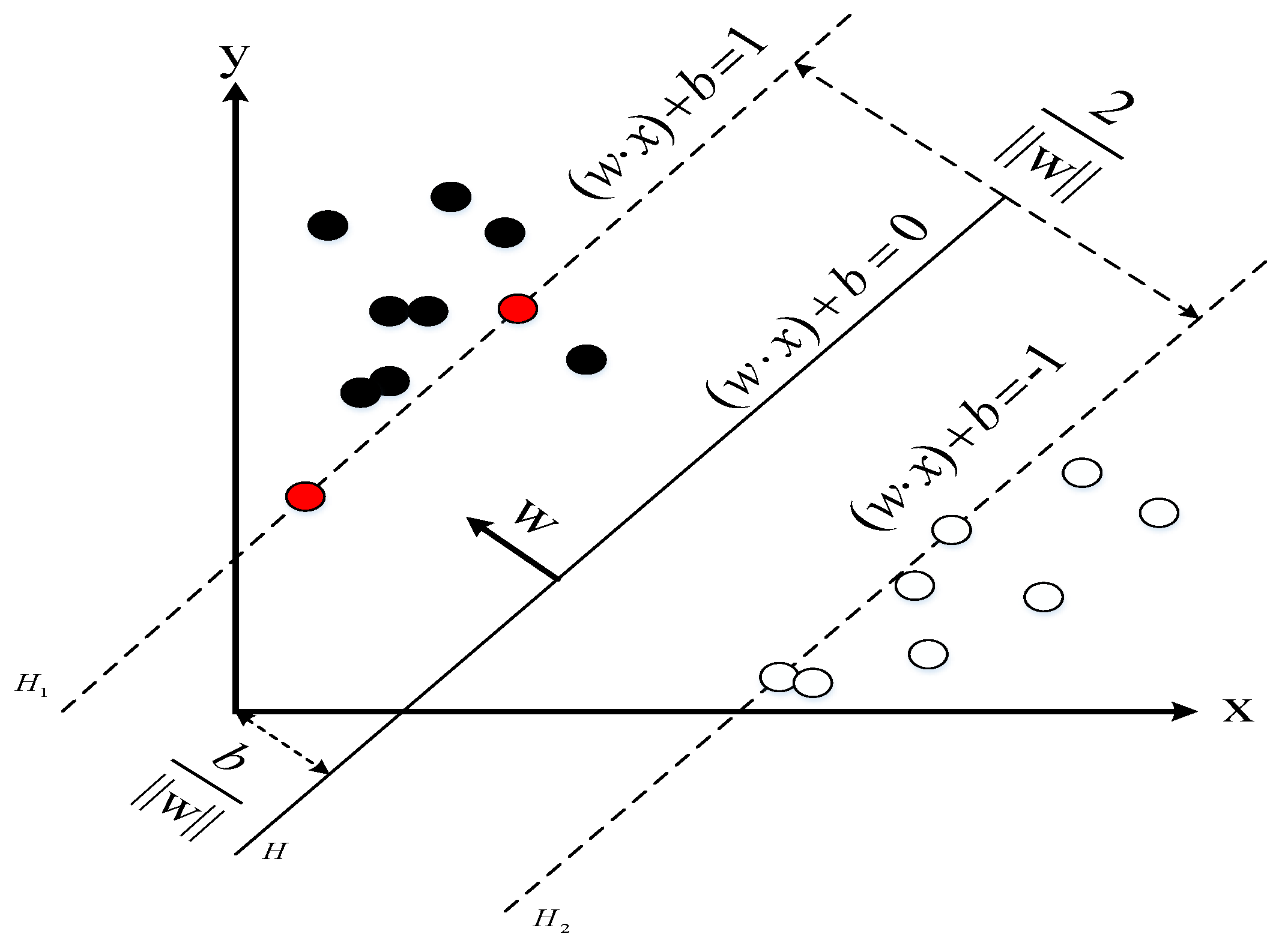
The core idea of the SVM is to find the optimal hyperplane that effectively separates different classes of samples in a feature space. In the case of linear separability, a hyperplane exists that perfectly separates two classes of samples and maximizes the margin, as shown in
Figure 2.
The training set is set to the following form:
represents the input feature vector, and represents the corresponding class label.
The hyperplane can be represented by a linear equation, , where w is the weight vector, x is the feature vector, and b is the bias. For any sample point (, ), the relationship between its class label and the hyperplane can be expressed as .
When the training data are linearly inseparable, a non-linear SVM can be learned by using the kernel function to transform the data and combining it with the margin maximization method. The main components include margin maximization, kernel functions, and the solution of the SVM.
2.2. Margin Maximization
The objective of the SVM is to ascertain a hyperplane that maximizes the margin, that is, the distance between samples of different classes. The distance between two different samples and the hyperplane is defined as the sum of the distances from each sample to the hyperplane. The optimization problem to maximize the distance can be formulated as a convex optimization problem.
The norm of the weight vector, denoted as , represents the magnitude of the weight vector, while represents the bias term. The label of the i-th sample point is denoted as , and the corresponding feature vector is denoted as . The objective of the optimization problem is to maximize the margin, which refers to the distance between the hyperplane and the two class sample points. Maximizing the margin helps improve the generalization ability of the classifier and its accuracy for new samples.
Meanwhile, the constraint ensures that each sample point is classified on the correct side. These constraints require all sample points to meet the correct classification requirements, thereby ensuring that the margin is not affected by misclassified samples.
2.3. Kernel Function
In practical applications, the data may be linearly non-separable, making it impossible to directly use a linear hyperplane for classification. To address this issue, the concept of kernel functions is introduced to map the data to a higher-dimensional feature space, making them linearly separable in the new feature space.
A kernel function is a function used to calculate the inner product between two sample points in the feature space. Common kernel functions include linear kernels, polynomial kernels, and radial basis function (RBF) kernels. By introducing kernel functions into the optimization problem of the SVM, non-linear decision boundaries can be obtained. For linearly non-separable cases, we can modify the optimization problem to the following form:
In the above formula, the constraint condition is softened by introducing slack variables to allow some samples to be misclassified. With , the slack variables, , represent the degree to which the training set is incorrectly classified. A larger slack variable indicates a higher degree of misclassification.
2.4. Solving the Support Vector Machine
The optimization problem of the SVM is a convex optimization problem, which can be transformed into a dual problem through Lagrange duality.
By constructing the Lagrange function:
where
is the Lagrange multiplier vector, the dual problem can be formulated as follows:
Solving the dual problem yields the optimal weight vector, w, and the bias term, b. In addition, according to the KKT (Karush–Kuhn–Tucker) conditions, only the Lagrange multipliers of the support vectors, , are non-zero, and they are located on the margin boundary, which determines the position of the optimal hyperplane.
In the practical association of AIS and radar track data, optimization algorithms such as SMO (Sequential Minimal Optimization) and QP (Quadratic Programming) are used to solve the dual problem and obtain the optimal solution for the support vector machine. In the context of ship radar and AIS track data association, the SVM demonstrates effective handling of high-dimensional and complex data, thereby enhancing the accuracy and reliability of vessel perception data association.
3. Trajectory Characteristic Calculation
Track characteristics denote the meaningful information extracted from various data sources, such as ship radar and AIS, which aid in the association of track data and the understanding of ship movement patterns. When calculating track characteristics, it is essential to preprocess the ship’s movement data and extract relevant characteristics. This preprocessing involves tasks like data cleaning, denoising, and handling missing data to guarantee the accuracy and completeness of the input data. Subsequently, by extracting features like speed, direction, turning rate, acceleration, and trajectory similarity from ship radar and AIS data, a feature vector representing the ship’s trajectory can be established. The following content explains the method of constructing each characteristic.
3.1. Trajectory Length Difference Characteristics
The utilization of the characteristics of length difference between radar tracks and AIS tracks aims to compare any discrepancies in the length of target trajectories captured by the two distinct data sources. By calculating the overall lengths of the radar track and the AIS track, the consistency of the target trajectory information across the different data sources can be evaluated. The length difference characteristic,
Lendiff, is expressed by the following formula:
where
Len(Radar_Trajectory) represents the length of the radar trajectory sample within a certain time span and
(AIS_Trajectory) represents the length of the AIS trajectory sample within a certain time span. If the difference in length between radar and AIS trajectories is small, this indicates that the target observed by the two data sources is more likely to be the same target, and vice versa. The length difference feature serves as a valuable indicator in detecting variations in trajectory length between radar and AIS data, which, in turn, aids in determining whether a target is associated with both data sources.
3.2. Course Difference Characteristic
Course denotes the direction of a ship’s movement trajectory relative to the ground, and we exclusively utilized course over ground for our analysis. The characteristics of course differences between radar tracks and AIS tracks are employed to compare any discrepancies in the course of targets observed by the two distinct data sources. By quantifying the difference between the average courses of radar tracks and AIS tracks, we can evaluate the consistency of target course information across diverse data sources. The course difference characteristic,
, can be expressed by the following formula:
where Course(Radar_Trajectory) signifies the course of the radar trajectory and Course(AIS_Trajectory) denotes the course of the AIS trajectory. If the difference in course is minimal, this implies that the target detected by the two data sources is highly likely to be the same target. Conversely, significant differences in the course information could indicate inconsistencies.
3.3. Average Acceleration Difference Characteristics
The characteristics comparing the average acceleration difference between radar tracks and AIS tracks are employed to analyze any discrepancies in the acceleration of targets detected by the two distinct data sources. Acceleration pertains to the rate of change in ship target speed with respect to time, and the acceleration range varies among different ships. During the construction of the dataset, we standardize the sample length to align with the temporal span of three AIS data points, ensuring consistency across samples. Consequently, the initiation time for calculating acceleration corresponds to the timestamp of the first AIS data point, while the termination time corresponds to that of the third AIS data point. Then, the average acceleration of AIS and radar data is computed within this designated timeframe. By calculating the difference between the average acceleration of radar track points and AIS track points, we can assess the consistency of target acceleration information across diverse data sources. Acceleration difference characteristics, Avg_Accelration, can be expressed by the following formula:
where
represents the acceleration of radar trajectory point
,
represents the acceleration of AIS trajectory point
,
n is the number of data points in the radar trajectory, and
m is the number of data points in the AIS trajectory. If the average acceleration difference is small, this indicates that the target accelerations observed by the two data sources are relatively consistent, indicating that the two observed trajectories are likely to be from the same target.
3.4. The Distance Difference in Starting Positions
The characteristics of the initial-position distance differences between radar tracks and AIS tracks are employed to compare any discrepancies in distance between the starting positions of targets observed by the two distinct data sources. By quantifying the differences in the distance between the initial points of radar tracks and AIS tracks, we can evaluate the consistency of targets’ initial-position information across diverse data sources. The distance difference characteristics of the starting position can be expressed by the following formula:
where
Pstart_Radar represents the starting-position point of the radar trajectory and
Pstart_AIS represents the starting-position point of the AIS trajectory. If the initial-position distance difference is small, this indicates that the target’s starting positions observed by the two data sources are relatively consistent, indicating that the two observed trajectories are likely to be from the same target.
3.5. The Distance Difference in End Positions
The feature of the end-position distance difference between radar tracks and AIS tracks serves as a crucial metric to compare the variance in the distance between the end positions of a target tracked by the two distinct data sources. By quantifying the distance difference between the end points of a radar track and an AIS track, we can assess the conformity of the target’s end-position information across different data sources.
where
Pend_Radar represents the end point of the radar trajectory and
Pend_AIS represents the end point of the AIS trajectory. If the end-position distance difference is small, this indicates that the target’s starting positions observed by the two data sources are relatively consistent, indicating that the two observed trajectories are likely to be from the same target.
3.6. Dynamic Similarity Characteristics
Dynamic time warping (DTW) is a method used to compare the similarity between two time series, which is widely applied in trajectory feature calculation. By treating a radar trajectory and an AIS trajectory as time series, the similarity between them can be calculated using the DTW algorithm, which allows us to quantitatively measure the dynamic similarity between the two trajectories.
Given two time series of radar and AIS trajectories, X = {x_1, x_2, …, x_m} and Y = {y_1, y_2, …, y_n}, where x_i and y_j represent the elements at timepoints i and j, respectively, firstly, construct an m x n cumulative distance matrix D, where D[i][j] represents the distance between the first i elements of sequence X and the first j elements of sequence Y. This distance can be calculated based on Euclidean distance metrics.
Secondly, compute the optimal path through dynamic programming to find the best alignment between sequence X and sequence Y.
where dist(x
i, y
j) denotes the distance between the sequence elements x
i and y
j. Finally, the DTW similarity between sequence X and sequence Y can be obtained by accumulating the lower-right element, D[m][n], of the distance matrix, D.
The primary advantage of DTW similarity lies in its ability to handle scenarios in which the lengths of time series are inconsistent and the speeds vary. In ship trajectory analysis, the speeds of ships may vary and the sampling frequencies of radar and AIS data may differ, leading to a mismatch between the two trajectories in the time dimension. The DTW algorithm utilizes dynamic programming to determine the optimal time alignment, effectively addressing these challenges and enabling more accurate similarity assessments.
This characteristic holds a crucial role in ship trajectory matching and association problems. By comparing the DTW similarity among diverse target trajectories, it aids in determining whether the radar and AIS data correspond to the identical ship target, thereby facilitating data association and consistency analysis.
4. Trajectory Dataset Construction
The aim of trajectory dataset construction is to extract the trajectory characteristics, as previously described, from labeled radar and AIS trajectory data. By extracting these features from labeled radar and AIS trajectory data and creating positive and negative samples, we can effectively train an SVM classifier, which facilitates the automatic classification and association of unlabeled data. These samples include both positive and negative instances, with positive samples comprising radar and AIS trajectory features labeled as the same target and negative samples consisting of radar and AIS trajectory features labeled as different targets. To maintain sample consistency, we standardized the sample length to correspond to the time span of three AIS data points. In the end, to address the issue of imbalanced distribution between positive and negative samples, we conducted imbalanced preprocessing to create the final dataset for model training.
4.1. Data Preprocessing
The AIS data of ships in a navigation environment are collected by the on-board AIS terminal, and then the location information of surrounding ships is extracted through protocol analysis. Due to the quality problem of AIS data, they usually need to be polished in historical data analysis. However, to mimic real-time scenarios, in which AIS reports sent from other ships are decoded and applied for association directly, raw AIS data are collected in the dataset construction. When vessels are not equipped with an AIS device, they can only be detected by radar. And, in data association, radar data will not match any AIS data. Therefore, track data from radar will be used for collision avoidance and radar data will be employed to build the negative samples.
Radar data preprocessing mainly includes shoreline elimination, connected component detection, and coordinate transformation. Firstly, to acquire radar targets, it is necessary to eliminate shorelines from the original radar images to obtain radar images solely containing the navigation areas of ships. Eliminating shorelines can remove the influence of riverbank objects on radar target detection. Based on the acquired shoreline positions, the intersection of the radar image and the area enclosed by the shoreline can be taken to eliminate the shoreline.
Subsequently, connected component detection is performed on these images to extract the targets of ships. In this paper, the two-pass scanning method [
22] was chosen for connected component detection. Through two scans, the connected components in an image can be detected, thereby identifying the radar targets within these connected components, as shown in
Figure 3. Then, ship objects are filtered according to the pixel values of each of the connected components.
Finally, in the domain of waterway transportation, the trajectory data generated by radar and AIS exhibit different data formats, which requires the transformation of coordinates. The conversion of radar polar coordinates to AIS coordinates fundamentally involves transforming the geodetic coordinate system into the polar coordinate system. The radar coordinate system operates in a polar fashion, with the radar device as its origin, measuring both distance,
, and rotational angle,
. Meanwhile, AIS target position data
are originally in the form of longitude and latitude in the geodetic coordinate system. Therefore, to integrate AIS and radar data effectively, conversion from the polar coordinates of radar to geodetic coordinates is necessary, as demonstrated by the equation below:
where (lon_r, lat_r) denote the geodetic coordinates of the radar data, (lon_o, lat_o) denote the coordinates of the radar device, θ represents the relative angle, d signifies the radar detection distance, and R denote the radius of the Earth.
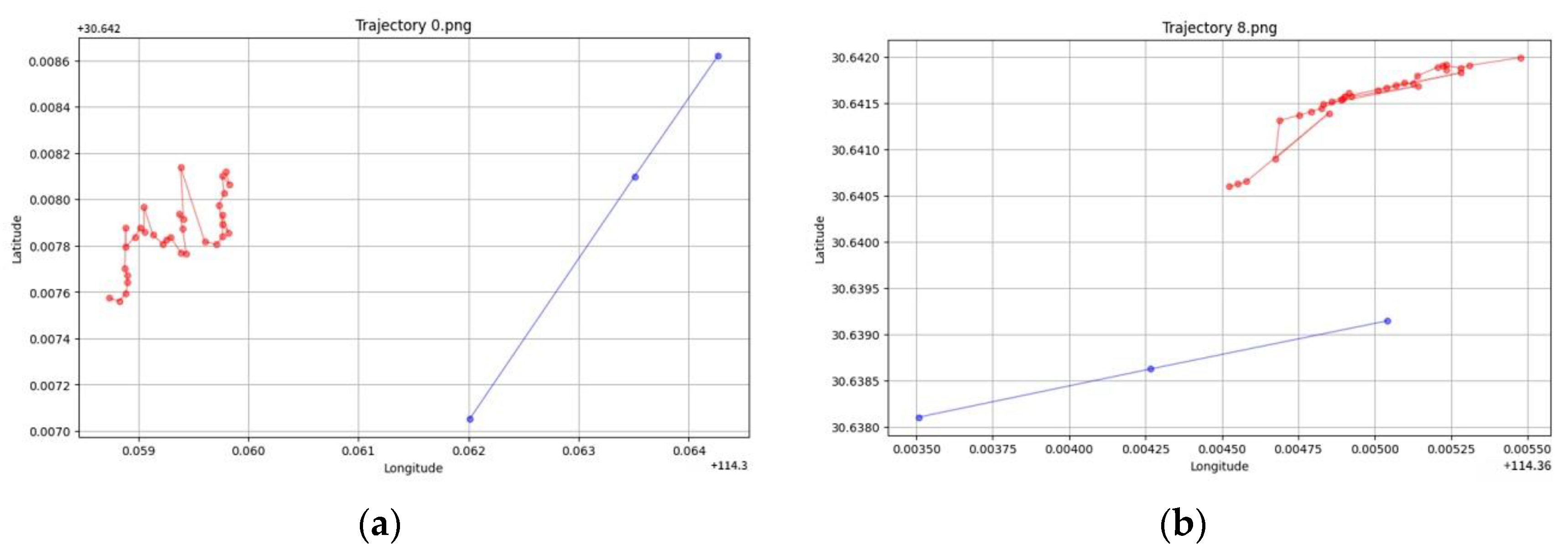
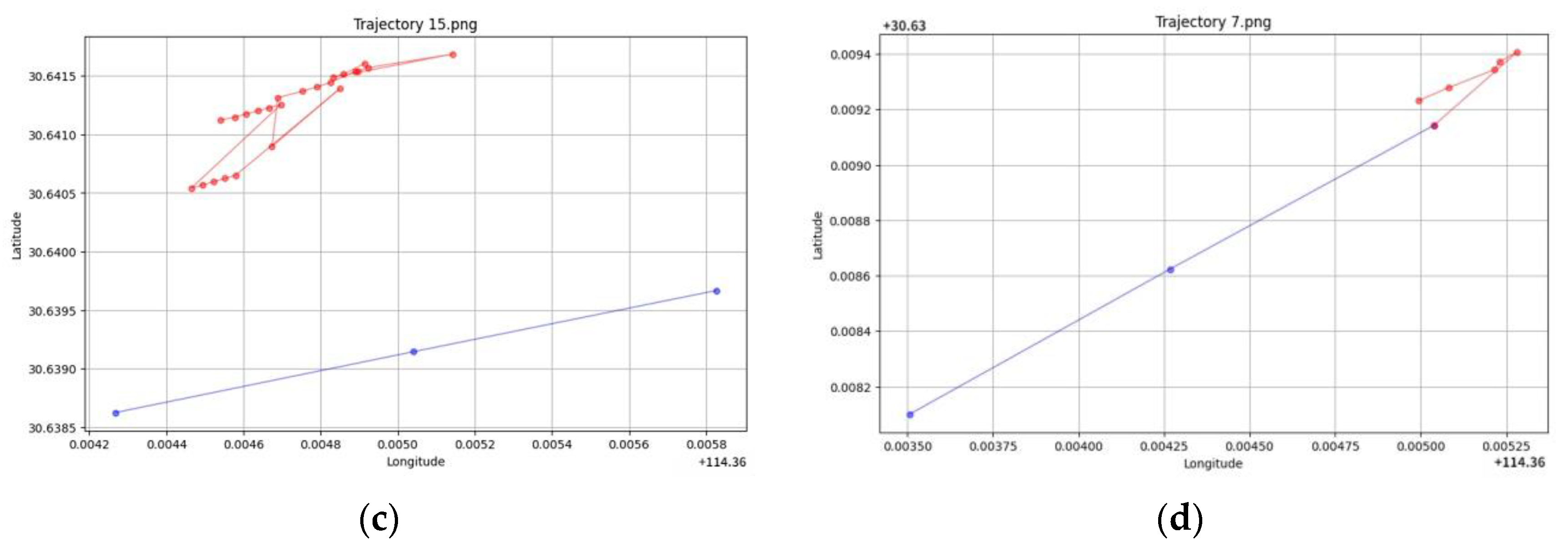
4.2. Positive Sample Construction
The process of constructing positive samples aims to establish a feature model for the target vessel, allowing the radar and AIS trajectory features belonging to the same target to be correctly associated. The specific steps are as follows:
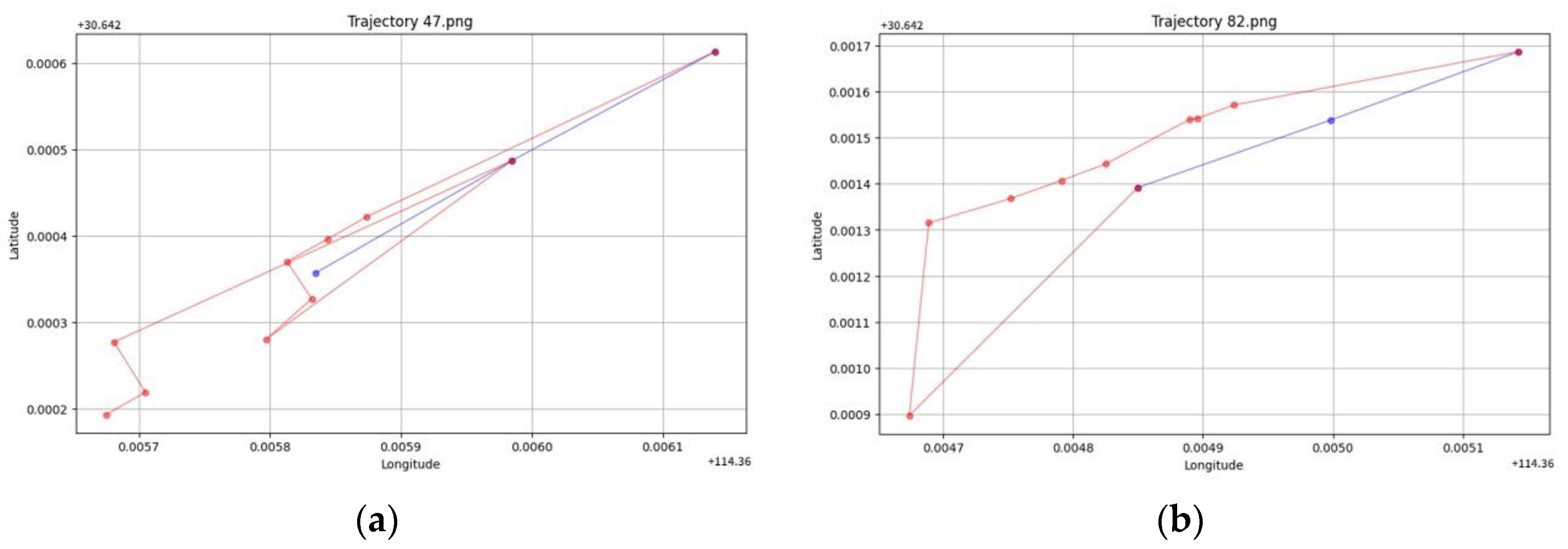
Step 1—Data Preparation: Initially, manual labeling of radar and AIS trajectory data is performed. These data encompass vessel motion information along with labeling information, indicating which radar and AIS trajectories correspond to the same vessel. For each pair of radar and AIS trajectories labeled as the same target, they are combined to form a positive sample trajectory pair, facilitating subsequent trajectory feature calculations. Positive sample trajectories are illustrated in
Figure 4.
Step 2—Time Alignment: Due to potential differences in the sampling frequency of radar and AIS data, there may be time discrepancies in the sample’s time dimension. To ensure data continuity and consistency, time alignment is carried out when constructing positive samples. Typically, the radar’s sample length is set to match the time span of three consecutive AIS data points, which helps mitigate issues related to inconsistent time intervals.
Step 3—Feature Extraction: Trajectory features, such as distance differences, course differences, and average acceleration differences, are extracted from radar and AIS data. These features reflect crucial characteristics of vessel motion, aiding in the establishment of ship identification and association models.
Step 4—Sample Labeling: For each constructed positive sample, a label of “1” is assigned, indicating that they belong to the same target vessel. These labels serve as training data for supervised learning, assisting the model in comprehending the characteristics of the target vessel.
4.3. Negative Sample Construction
The process of negative sample construction aims to establish a feature model capable of distinguishing between different vessels. Negative samples are composed of radar and AIS trajectory features labeled as different targets, assisting the model in understanding the trajectory differences between various vessels from AIS and radar data. The detailed procedure for negative sample construction is as follows:
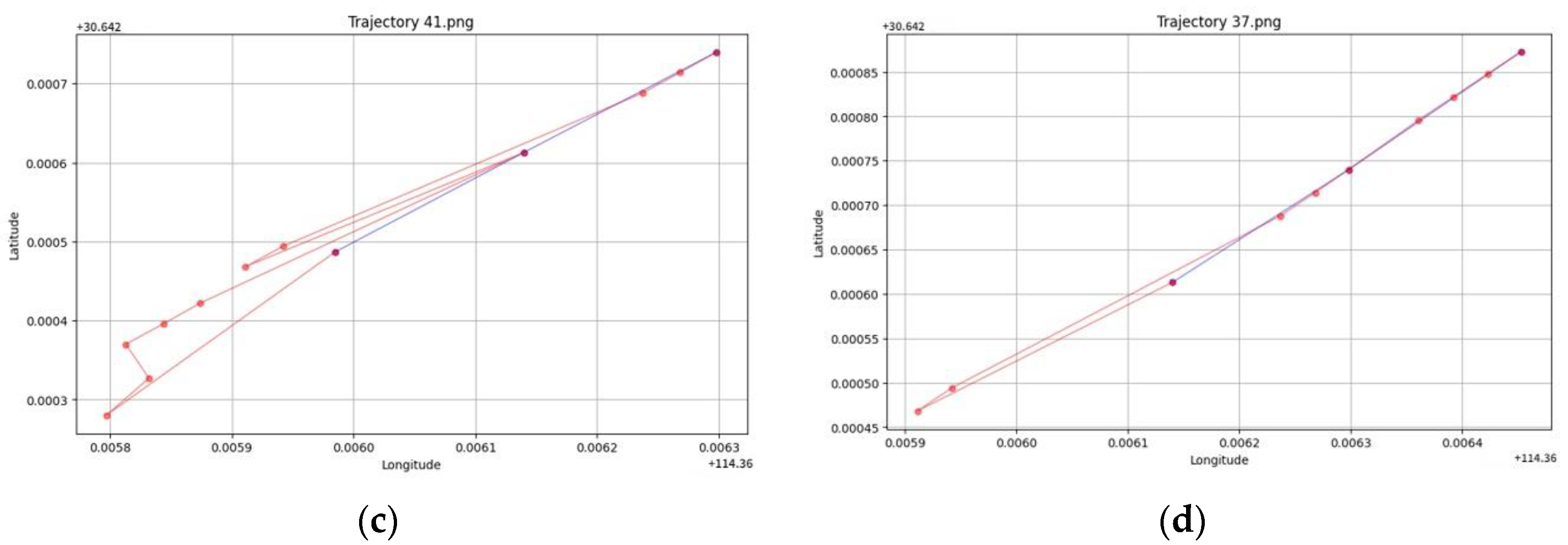
Step 1—Data Preparation: In contrast to the positive sample construction process, we initially select radar and AIS trajectory data that are not labeled as the same target during the same time interval. These datasets contain vessel motion information and labeling information, indicating which radar and AIS trajectories correspond to different target vessels. For each pair of radar and AIS trajectories labeled as different targets, they are combined to form a negative sample trajectory pair. Negative sample trajectory pairs are illustrated in
Figure 5.
Step 2—Time Alignment: Similar to the positive sample construction process, time alignment is crucial for radar and AIS trajectories to guarantee the synchronization of heterogeneous data within a consistent temporal interval.
Step 3—Feature Extraction: Similar to the process of constructing positive samples, trajectory features, such as distance differences, course differences, and average acceleration differences, are extracted from radar and AIS trajectory data. These features serve to characterize the differences in AIS and radar data between different vessels.
Step 4—Sample Labeling: For each constructed negative sample, a label of “0” is assigned, indicating that the features of this negative sample trajectory pair belong to different vessels.
4.4. Imbalanced Preprocessing
The process involves combining the constructed positive sample set with the negative sample set to create a comprehensive dataset. In tasks associated with associating ship radar and AIS data, the number of positive samples representing the same target vessel trajectories is relatively limited, while the number of negative samples corresponding to different target vessels is more substantial. Given that the SVM algorithm is significantly affected by sample distribution within the dataset, this imbalance can potentially lead to a reduction in the model’s performance during both training and testing phases. This is primarily because the model tends to favor predicting the class with a higher sample count while neglecting the one with fewer samples.
To guarantee the precision and resilience of model training, it is paramount to ensure a balanced distribution of both positive and negative samples across the entire dataset. In this research, we harness the SMOTE (Synthetic Minority Over-Sampling Technique) algorithm to synthesize additional samples, thereby augmenting the minority class representation and mitigating the imbalance in sample category distribution. The generation of these synthetic samples occurs within the feature space and leverages the inherent similarity among samples in the minority class, thereby improving the original data’s class distribution imbalance. Consequently, this effectively addresses the problem of sample category imbalance, enhancing the model’s performance and generalization capabilities.
5. Experiments and Results
5.1. Data Sources
In our experiments, we employed radar and AIS trajectory data collected from the perception-integrated system installed on the vessel “HANG DAO 1 HAO” within the Yangtze River inland waterway. The shipborne perception system incorporates SIMRAD solid-state radar, which is widely used in maritime field. The detection range of the radar is between 1/32 nm and 36 nm. The AIS device used in the system meets the relevant standards of AIS Class B and can receive data related to ship navigation safety in real time. The dataset encompasses radar and AIS data for various target vessels, along with corresponding labeling information, as shown in
Figure 6 and illustrated in
Table 1. In the figures, own ship is the “HANG DAO 1 HAO” vessel with the MMSI 413835537, and the straight lines in front of the vessel icons represent their headings. This dataset was collected under sunny weather conditions with high visibility. The AIS data contained data decoded from AIS reports with static and dynamic information. Radar data included radar IDs, labeled MMSIs (Maritime Mobile Service Identities), and the other features were the same as in the AIS dataset, which had 9307 records with labels. From this dataset, we extracted several sample features, including distance differentials, course differentials, average acceleration differentials, starting-point distance differentials, end-point distance differentials, and DTW similarity features. To facilitate our experiments, we divided the constructed dataset into training and testing sets in a 7:3 ratio, allowing for comprehensive testing and evaluation of our proposed methods. This division ensured the independence of the test data from the training data, enabling us to assess the effectiveness and performance of our approaches accurately. The utilization of real-world ship monitoring data from the Yangtze River inland waterway added authenticity and applicability to our experimental framework, contributing to the robustness and relevance of our research outcomes.
5.2. Evaluation Criteria
Experimental evaluation metrics were utilized to assess the performance of the SVM model in the task of associating ship radar and AIS trajectories, specifically its ability to accurately identify AIS and radar trajectories as belonging to the same vessel. The primary experimental evaluation metrics were precision, recall, and F1 score.
Precision: Precision refers to the proportion of samples that are predicted as “true” by a model and are indeed true positives. It is particularly relevant when dealing with binary classification problems, where the goal is to classify instances into one of two classes, typically referred to as the positive class and the negative class. Here, a high precision value indicates that the model is good at identifying the heterogeneous data belonging to one vessel and does not make many false-positive errors.
Recall: Recall refers to the ratio of positive samples correctly predicted by a model to true-positive samples. Specifically, in the present study, recall is defined as the number of true-positive classifications (correctly identified instances of data from the same vessel) divided by the sum of true positives and false negatives. It indicates the model’s capacity to capture and correctly classify data instances that truly belong to the same vessel, which is essential in vessel tracking, navigation, and various maritime applications. A high recall score means that the model is effective at finding and classifying most of the heterogeneous data belonging to the same vessel, reducing the risk of missing important information.
F1 Score: The F1 score is a metric used in classification tasks, including the classification of AIS and radar data belonging to one vessel [
23]. It is a valuable measure that combines both precision and recall into a single value to provide a more comprehensive evaluation of a model’s performance, especially in scenarios with imbalanced class distributions. The F1 score is calculated as follows:
F1 scores range from 0 to 1, with a high F1 score suggesting, here, that the model achieves a balance between correctly classifying data as belonging to one vessel while minimizing the risk of missing relevant data points. Therefore, we can conduct a comprehensive evaluation of the model’s performance on the ship radar and AIS trajectory association task in the test dataset using F1 scores. High precision, recall, and F1 score will substantiate the capability of our proposed method to accurately discern whether AIS and radar trajectories pertain to the same target.
5.3. Results
In inland waterways, where there is a high density of traffic flow, frequent cross encounters, and substantial diversity in vessel trajectories, the challenge of data association becomes particularly intricate and complex. Therefore, we conducted experiments categorized into four groups: vessels moving with the same heading, vessels moving close together with the same heading, vessel encounter scenarios, and multiple vessel encounter scenarios. These experiments allowed us to conduct a comparative analysis of the performance of the ship radar and AIS trajectory data association method based on the SVM in different scenarios.
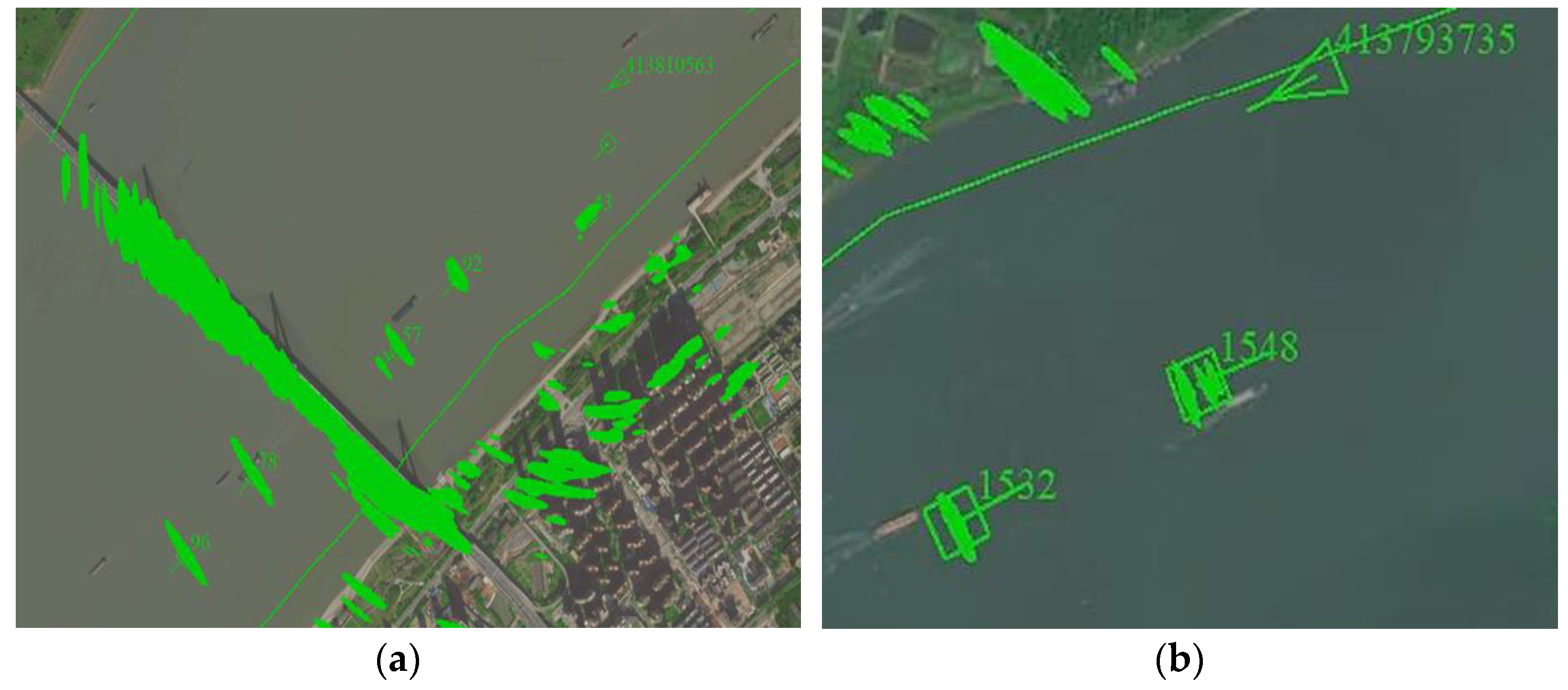
- (1)
Vessels moving with the same heading
The purpose of this experimental group was to explore situations in which vessels move in the same direction, observed by both radar and AIS. Specifically, we selected two typical situations within this group for analysis. We extracted and processed the data to obtain a total number of 174 trajectory samples for further analysis. In this situation, the vessels’ movements are in the same direction, albeit with noticeable distances between them, as illustrated by target 92 and target 57 in
Figure 7a and target 1532 and target 1548 in
Figure 7b. The experiment aimed to confirm the effectiveness and accuracy of our approach in addressing these same-direction forward- and backward-movement scenarios.
An F1 score of 0.96 signifies a balanced trade-off between precision and recall delivering accurate classification results. The model effectively discriminates between the radar and AIS trajectories of the target vessels, aligning precisely with the actual labels.
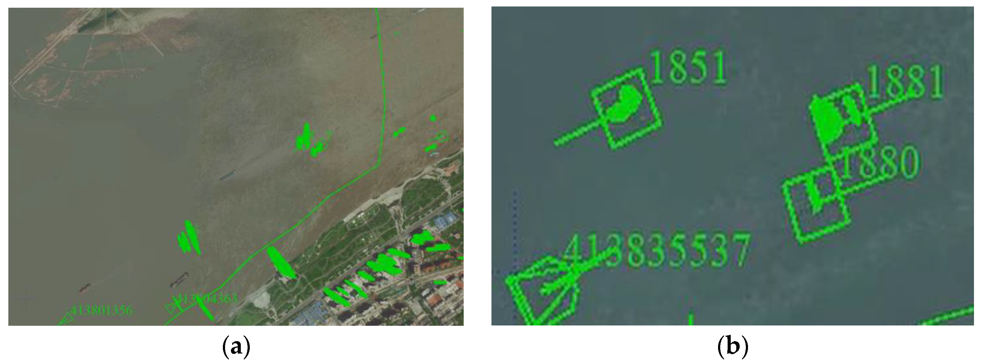
- (2)
Vessels moving close together with the same heading
This experimental grouping was designed to replicate scenarios in which vessels closely follow the same course and are ready to overtake in both radar image and AIS data. Specifically, we selected two typical situations within this group for analysis. We extracted and processed the data to obtain a total number of 415 trajectory samples for further analysis, as illustrated by target 7 and target 8 in
Figure 8a and target 1880 and target 1881 in
Figure 8b. In this case, multiple vessels are navigating near each other while maintaining a consistent direction of movement. This suggests a scenario in which the vessels may be in the process of overtaking one another, with one vessel gradually moving past another while maintaining a similar course. In these circumstances, the radar and AIS trajectories of the target vessels displayed distinct temporal and spatial similarities and were characterized by minimal differences in distance, heading, and speed.
Through calculations, we obtained an F1 score of 0.95. These results signify the performance of the data association method in the scenarios in which vessels 7 and 8 were moving close together in the same direction.
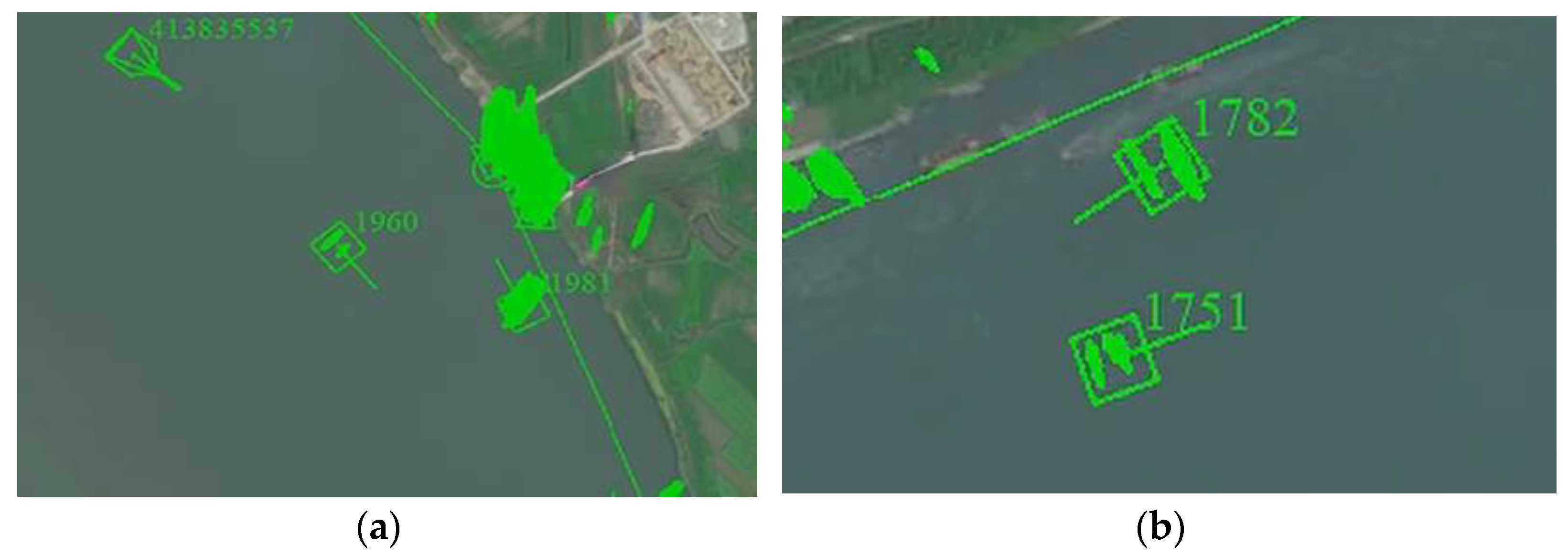
- (3)
Vessel encounter scenarios
In this group, we considered scenarios in which target vessels encounter each other in both radar image and AIS data. An encounter refers to a situation in which vessels approach each other in close proximity or along intersecting paths. Specifically, we selected two typical situations within this group for analysis. We extracted and processed the data to obtain a total number of 77 trajectory samples for further analysis. In such cases, the trajectories of the target vessels may exhibit significant differences in terms of distance and heading, as illustrated by the trajectories of vessels 1960 and 1981 in
Figure 9a and target 1751 and target 1782 in
Figure 9b. This experiment was designed to evaluate the performance of our method in situations involving vessel encounters.
By computation, an F1 score of 0.98 was obtained, indicating that the proposed method for associating ship radar and AIS trajectory data performs accurately in scenarios in which vessels encounter each other.
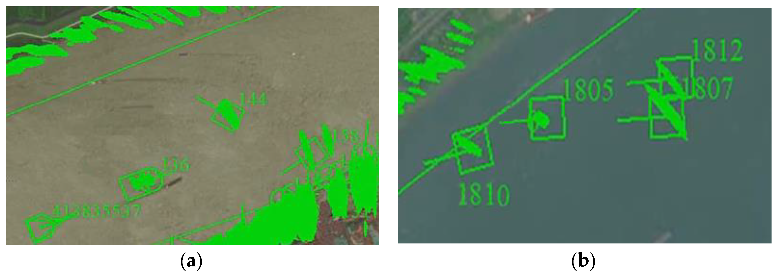
- (4)
Multiple vessel encounter scenarios
In this set of experiments, we explored scenarios in which multiple vessels simultaneously encounter one another in both radar image and AIS data. Specifically, we selected a typical situation within this group for analysis. We extracted and processed the data to obtain a total number of 230 trajectory samples for further analysis. Multiple-target association requires simultaneous associations across multiple sets of radar and AIS trajectories, as depicted by the examples involving vessels 158, 144, and 136 in
Figure 10a and vessels 1805, 1807, 1810, and 1812 in
Figure 10b. The experiments aimed to investigate the applicability and efficiency of our proposed association method in multi-target scenarios.
Through calculations, we obtained an F1 score of 0.97. These results confirmed the performance of the classifier-based association method in the scenario involving vessels encountering one another, which indicates the model’s ability to distinguish between different vessels in multiple vessel encounter scenarios.
6. Discussion
We conducted a comparison with the nearest-neighbor method to provide a more comprehensive evaluation of our classifier approach. The comparison results are presented in
Table 2,
Table 3,
Table 4 and
Table 5, which detail the evaluation metrics for the different scenarios. For scenarios involving vessels moving with the same heading (
Table 2,
Table 3 and
Table 4), both our classifier approach and the NN method demonstrated high precision, recall, and F1 score values. In the multiple vessel encounter scenarios (
Table 5), our classifier approach consistently achieved higher precision, recall, and F1 score values than the NN method, highlighting its robustness and effectiveness in identifying vessel encounters.
Our analysis focused on a representative set of data collected by on-board perception systems in several classical scenarios, including overtaking and encounters. In these simpler scenarios, both existing NN models and the proposed model exhibited satisfactory trajectory association performance. This is attributable to the relatively straightforward nature of these scenarios, in which ship movement patterns are more uniform and thus easier for models to associate. However, when confronted with more complex scenarios, such as multiple vessel encounters, the proposed method demonstrated its distinct advantage. In multiple vessel encounter scenarios, multiple vessels interact within a limited space, resulting in more intricate and variable trajectory characteristics. In the multiple vessel encounter scenario (
Table 5), the nearest-neighbor method exhibited a precision, recall, and F1 score of 0.86. Compared to our classifier approach, the NN method demonstrated a lower performance across all evaluation metrics in this scenario. The NN method, which relies solely on proximity-based matching, may struggle to accurately identify and associate trajectories in such dense and intricate scenarios. And this is attributable to the complexity of the situation, in which distinguishing between multiple overlapping vessel trajectories poses a challenge. In contrast, because it utilizes a comprehensive set of features derived from trajectory characteristics, which enable it to capture nuanced patterns and relationships in the data, our classifier approach ensures accurate identification of positive instances.
Overall, while both methods performed well, the results shown in
Table 5 highlight the superior performance of our classifier approach, particularly in scenarios involving multiple vessel encounters. Incorporating multiple trajectory characteristics to solve data association issues makes it more reliable than approaches like the NN method which just take trajectory distance into account. However, its accuracy relies heavily on the training dataset, which may not effectively generalize to complex or open-sea scenarios not adequately represented in the training data mainly obtained from an inland waterway. And as we focused on the association method for AIS and radar data, cases in which radar or AIS are not employed were not considered in this study. Furthermore, the data primarily originated from a single vessel’s perception system, and the scenarios selected were relatively limited, potentially affecting the model’s generalization capabilities. In future research, we aim to collect a more diverse and extensive dataset, encompassing data from various types of vessels, different weather conditions, and across diverse geographical locations. This will enhance the model’s performance and generalization.
Meanwhile, video sensors play a crucial role in enhancing vessel perception, especially in challenging visibility conditions and nighttime operations, where AIS and radar may fall short. After the inclusion of video, we can extend our approach to utilize target detection algorithms to identify vessels present in a video at first. Subsequently, coordinate transformation can be performed to align the coordinates of detected vessels with AIS and radar. Furthermore, leveraging the calibrated relationships between video targets and those identified by radar and AIS, positive and negative sample sets could be constructed for vessel trajectory features in video data. These sample sets will serve as the basis for training a data association classifier, enabling the correlation of vessel perception data from video, AIS, and radar sources. Sensor fusion techniques allow us to leverage the strengths of each sensor type while compensating for their individual limitations. By combining AIS, radar, and video sensor data, we can enhance the accuracy and reliability of vessel motion perception.
7. Conclusions
In this study, a trajectory characteristic-based SVM binary classifier approach is proposed to achieve effective association between ship radar image and AIS data. Based on the data captured from a perception system installed on a vessel named “HANG DAO 1 HAO”, we extracted trajectory characteristics of different vessels from radar and AIS data. Then, positive and negative training sets were constructed to feed them into the classifier for association analysis. The research results demonstrate that the trajectory characteristic-based SVM binary classifier excels in ship radar and AIS data association. Through a series of experiments that included two typical situations for each of the following: overtaking, encounters, and multi-target groups, which are common situations in inland waterway traffic contexts, this research substantiated the method, which achieved an F1 score greater than 0.95, with the aim of enhancing the precision and reliability of ship monitoring and navigation information.
In a future study, more diverse and extensive datasets will be collected to enhance the model’s performance and generalization. This could involve using data from different types of vessels, varying weather conditions, and different geographical locations. Moreover, the integration of data from other sources, such as CCTV or BEIDOU data, which have the ability to detect objects without radar or AIS data in challenging visibility conditions, will be applied to expand and compensate for the detection capacities of current ship monitoring and navigation. And in future work, data fusion methods, such as covariance intersection, will be implemented after data association to provide more accurate position information about surrounding vessels and enhance maritime situational awareness.


