Modelling the Dynamics of Outbreak Species: The Case of Ditrupa arietina (O.F. Müller), Gulf of Lions, NW Mediterranean Sea

Abstract

An outbreak species exhibits extreme, rapid population fluctuations that can be qualified as discrete events within a continuous dynamic. When outbreaks occur they may appear novel and disconcerting because the limiting factors of their dynamics are not readily identifiable. We present the first population hybrid dynamic model that combines continuous and discrete processes, designed to simulate marine species outbreaks. The deterministic framework was tested using the case of an unexploited benthic invertebrate species: the small, serpulid polychaete Ditrupa arietina. This species is distributed throughout the northeast Atlantic Ocean and Mediterranean Sea; it has a life cycle characterised by a pelagic dispersive larval stage, while juveniles and adults are sedentary. Sporadic reports of extremely high, variable densities (from <10 to >10,000 $ind.m^{-2}$) have attracted attention from marine ecologists for a century. However, except for one decade-long field study from the Bay of Banyuls (France, Gulf of Lions, Mediterranean Sea), observations are sparse. Minimal formulations quantified the processes governing the population dynamics. Local population continuous dynamics were simulated from a size-structured model with a null immigration–emigration flux balance. The mathematical properties, based on the derived hybrid model, demonstrated the possibilities of reaching an equilibrium for the population using a single number of recruits per reproducer. Two extrapolations were made: (1) local population dynamics were simulated over 180 years using North Atlantic Oscillation indices to force recruitment variability and (2) steady-state population densities over the Gulf of Lions were calculated from a connectivity matrix in a metapopulation. The dynamics reach a macroscopic stability in both extrapolations, despite the absence of density regulating mechanisms. This ensures the persistence of D. arietina, even when strong, irregular oscillations characteristic of an outbreak species are observed. The hybrid model suggests that a macroscopic equilibrium for a population with variable recruitment conditions can only be characterised for time periods which contain several outbreak occurrences distributed over a regional scale.

1. Introduction

Species populations fluctuate continuously, but the intervention of a discrete event, whether internal (e.g., reproduction, migrations) or external (e.g., heat waves, flooding, emersion/immersion cycles, harvesting), may disrupt the continuous dynamic causing step-wise change(s) of state. To an observer, this state change can appear sudden and unexpected [1]. This pattern of change characterises a population irruption or outbreak. Species outbreaks have complex dynamics with cycles that can be periodic or aperiodic and which may be triggered, or not, by an identified external factor [2]. They pose a major challenge in ecological theory because there is an apparent lack of regulation by density-dependence, food resources, or predation on the population which are the norm in finite systems [2]. Authors have looked for many different explanations for outbreaks, including periodicities in observed cycles [3], links to life history traits [4], and indirect disturbances in the trophic chain [5]. However, these have provided only partial explanations after outbreaks occur; their complexity has largely escaped predictive approaches (see review of knowledge gaps for the crown-of-thorns starfish [6]).

A plausible explanation for this lack of success is that the population dynamics models used are ill-suited to simulating the dynamics involved. Existing modelling techniques designed for population dynamics emphasise different features—size distribution, fecundity, continuous or discrete spatial distributions, interactions, etc.)—to the detriment of general aspects, and very few explicitly treat the interactions between a discrete event (the outbreak, per se) with the underlying continuous population dynamics. Hybrid model frameworks seem necessary to simulate ecological systems characterised by multiple scales of variations, especially for simulating population outbreaks. Hybrid models are commonly used in engineering problems (e.g., thermostats or car braking systems), but are much more rarely seen in ecology, possibly because of the difficulties to analyse their mathematical properties [7].

Our aim here is to formulate a simple hybrid model without any limitations and to explore if the dynamic of an outbreak can be represented from only the species demography, distribution observations, and information about environmental trends. A small, invertebrate species, Ditrupa arietina was selected to test the model with. It is widely distributed in soft substrates of coastal ecosystems in the northeastern Atlantic Ocean and the Mediterranean Sea (Figure 1; [8,9,10]. It has a pelagic, dispersive larval stage, with sedentary juvenile and adult forms. There are sparse reports of extremely high densities occurring throughout its distribution area (see review in [8]). Because this species does not have any economic value, nor does it directly affect human activities, detecting the negative impact of an outbreak is not used as a criterion (e.g., [11]). Instead the focus of this study is on the mathematical properties of the population dynamic to infer the population irruption pattern. D. arietina is an interesting example to treat because of all the different ways its population fluctuations have been interpreted as evidence of ecological processes, without the influence of management issues generated by other species’ outbreaks. The pattern of intermittent, patchy high densities has led to D. arietina being:

• included in a benthic index assemblage [12], used in European water quality assessments [13];
• interpreted as having a particular interest for carbon cycling [14] because they build an external tube made of CaCO₃;
• treated as an example of a spatially distributed metapopulation [15] in which the pelagic larval stage and hydrodynamic transport ensure dispersion and mixing at regional scales [16,17]. This highlighted possible links between climate patterns on hydrodynamic conditions that could modify the distribution of the species and its preferred habitat to different extents.

Two of these uses (i.e., 1 and 2, above) clearly depend on a quantitative understanding of the population dynamics involved, while the third use would be improved by an explicit treatment of the population irruption over the spatial domain. In each case, a better understanding of whether a population irruption is expected, or not, is important to the reliability of these uses.

The objective of this article is to quantify, from all available information, the population dynamics of D. arietina in the Bay of Banyuls-sur-Mer (France), emphasising the complexity of the dynamics that allows outbreaks to occur. For this, several related mathematical models were formulated: (1) to simulate the dynamics of the size-structured population of D. arietina in the bay, (2) to hindcast the dynamics of the population at scale of centuries, and (3) at the spatial scale of the Gulf of Lions (${10}^{3}k{m}^2$). The models are minimal and do not take into account any limitation functions. Their mathematical properties were studied to investigate conditions of persistence or extinction of the local population, and different hypotheses are discussed for local and regional scales by comparing simulations and observations from the Bay of Banyuls locality with other data collected throughout the Gulf of Lions [18]. This study is seen as a new starting point to producing better quantification of species’ outbreak episodes relative to other processes.

Figure 1. Study area in the context of the overall distribution of D. arietina occurrences along the northeastern Atlantic and Mediterranean coasts, post-1800. Data from: OBIS [10] (median year = 2006; 6696 instances in map area of 6765 total) and 20 additional locations from two new sources (Koehler [19], Hartley [8]). The violin plot shows the limited time range of the observations (>99% are from the past 70 years) and most of these are from surveys in Norwegian waters (5365 instances between 1990 and 2021). Banyuls Bay is at the extreme western edge of the study area, near the French–Spanish border. No population genetics studies on this species have been reported in the region shown.

Figure 1. Study area in the context of the overall distribution of D. arietina occurrences along the northeastern Atlantic and Mediterranean coasts, post-1800. Data from: OBIS [10] (median year = 2006; 6696 instances in map area of 6765 total) and 20 additional locations from two new sources (Koehler [19], Hartley [8]). The violin plot shows the limited time range of the observations (>99% are from the past 70 years) and most of these are from surveys in Norwegian waters (5365 instances between 1990 and 2021). Banyuls Bay is at the extreme western edge of the study area, near the French–Spanish border. No population genetics studies on this species have been reported in the region shown.

2. Materials and Methods

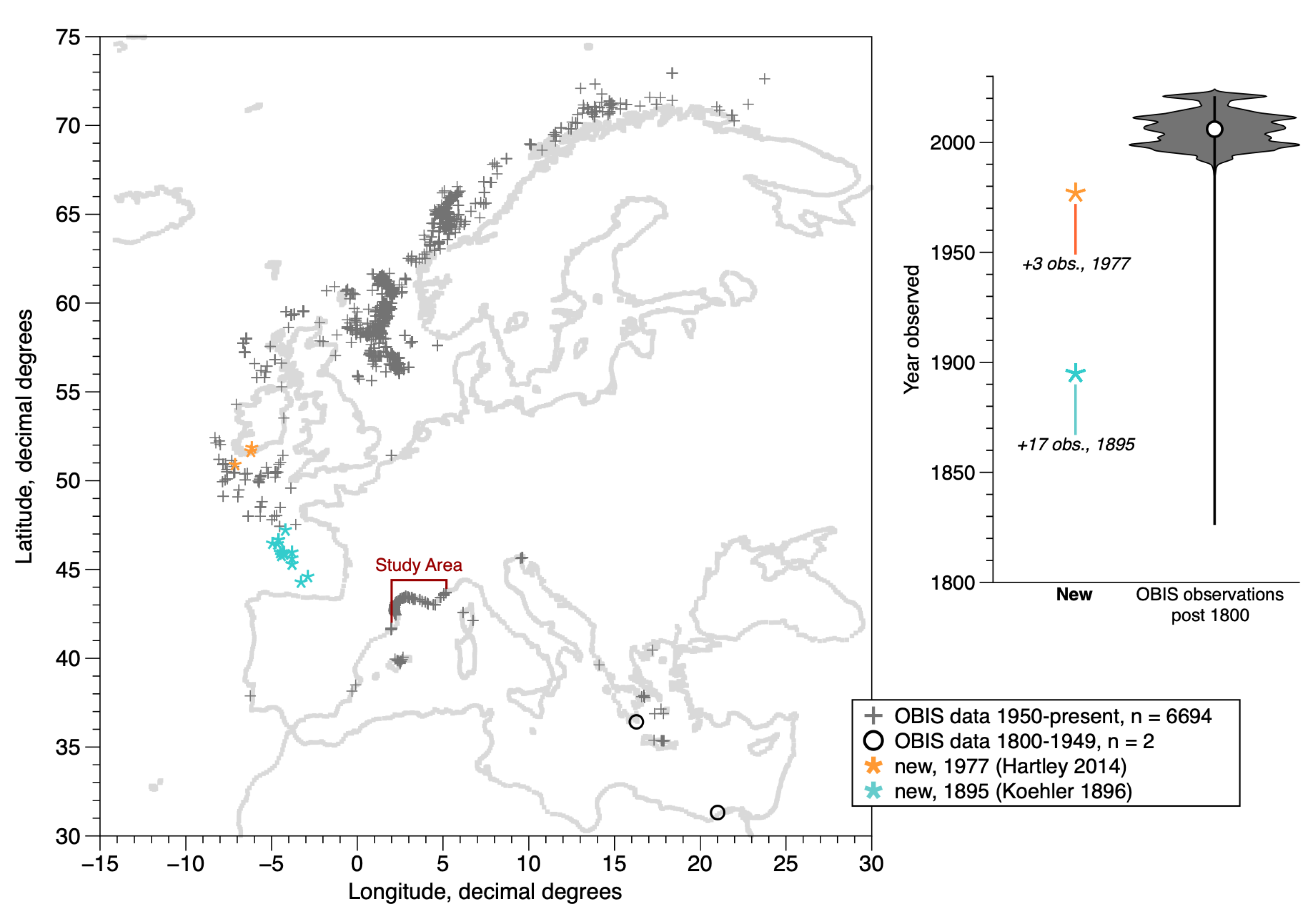
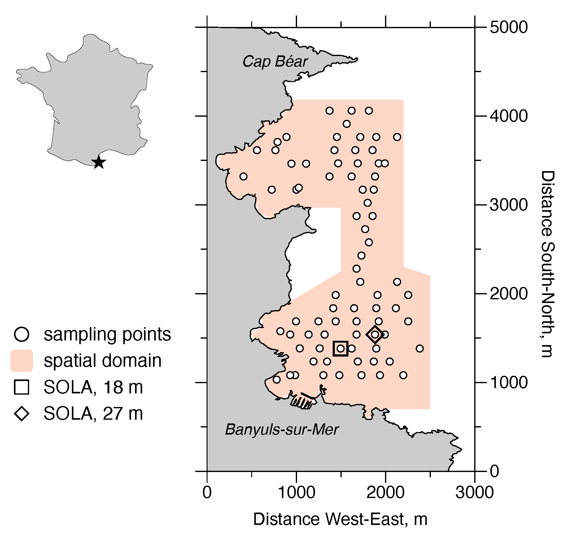
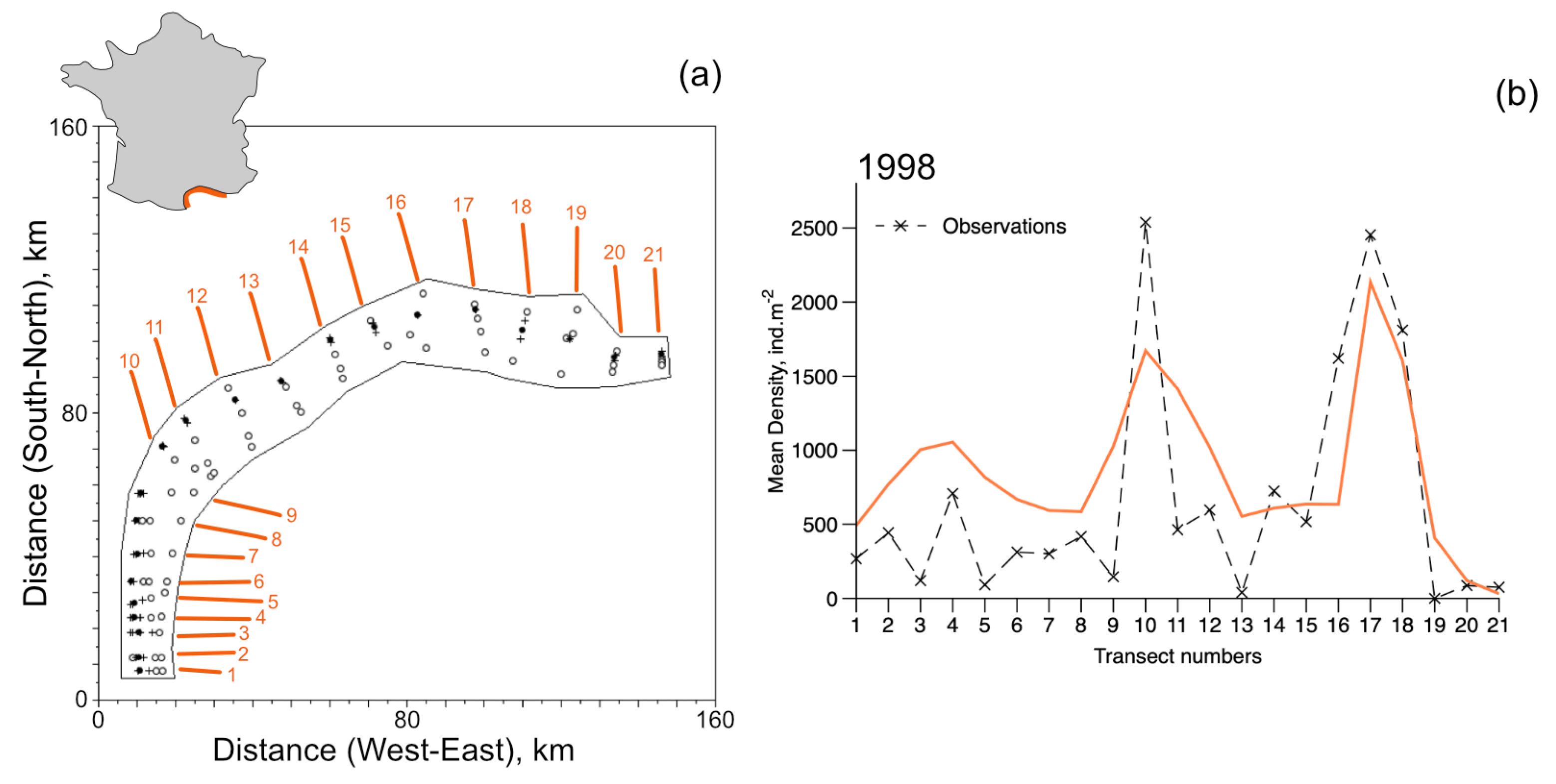
2.1. Brief Description of the Species Distribution and Field Studies

Ditrupa arietina is a short-lived (2 yr lifespan, post recruitment [20]) suspension feeder [21] with a distinctive conical tube shell (<60 $mm$ long) that lives on the surface of fine-grained sediment substrates instead of digging in. D. arietina occurs in shallow to moderate depths (generally <200 m) throughout the northeastern Atlantic and Mediterranean Sea (Figure 1). Most observations in the OBIS database [10] are recent; it is not possible to determine the fraction of live specimens or empty shells in these data. This is an issue because the organism is susceptible to transport by bottom currents under some hydrodynamic regimes [22] and shells are sometimes described as partly fossilised (e.g., [19]). The study area represented with the model is in the southern part of the distribution (Gulf of Lions; Figure 1). Three sources of data were available in the study area: a ten-year survey of the D. arietina population at one point in the Bay of Banyuls-sur-Mer, eight spatial surveys in the same bay during the same time period [1,16,20,23], and two large-scale benthic diversity surveys completed in the Gulf of Lions [18,24]. Two recent studies of benthic biodiversity [25,26] have also analysed these datasets.

The ecology of D. arietina was studied intensively in the 1990s and early 2000s in the Bay of Banyuls-sur-Mer, France, Gulf of Lions (42°30.00′ N; 003°08.50′ E; Banyuls Bay, hereafter). Banyuls Bay is a small open embayment situated at the southern end of the Gulf of Lions, near the French–Spanish border (Figure 2). Water renewal depends strongly on the local water circulation which is influenced by a specific wind regime [16]. The main water circulation outside the bay is oriented north–south, and the water depth increases from west to east. The isobath at $38m$ was used as a boundary for the bay at the eastern edge. The bay surface used in calculations is about $6k{m}^2$ (orange area, Figure 2) corresponds to a volume of ca. $0.15k{m}^3$. Sediments range from fine sands to muddy-sands (about 25% of particles with an equivalent diameter less than $40\mu m$).

Banyuls Bay hosts a high benthic species diversity [12] with low population densities [27]; population densities of dominant species rarely exceed 50 $ind.m^{-2}$. During a benthic macrofauna species survey in the early 1990s, D. arietina was found at very high densities of tens of thousands of individuals per square meter [1]. This caught the attention of researchers because the species had not been identified during a similar inventory carried out several decades earlier in the late 1960s [24,28]. The modelling uses observations collected from the field sampling campaign initiated in Banyuls Bay (Figure 2 after the high density observations [1]. During the nine-year time period (between June 1994 and June 2003) D. arietina population densities were recorded every two weeks at the permanent station in the bay (Figure 2, “SOLA”) [20]. The tube size (length of the straight axis between the opening and the opposite end of the tube, $mm$), biomass (flesh dry weight, in g), and the CaCO₃ biomass (in g), were measured on all post-metamorphosis individuals, after hand sorting [1,14,20]. The tube is assumed to be made only from calcite.

In addition to the biweekly sampling at one station, a series of synoptic spatial samplings of the population densities were conducted in the Bay eight times, between 1996 and 2003, for a set of 78 stations (Figure 2). The spatial samplings were analysed with standard geostatistics (quantification of variograms and interpolation on the sampling domain by point kriging; estimates made with GS+ software (v. 10, 2014, Gamma Design Software LLC, Plainwell, MI, USA) These distributions were then used to estimate the frequency distribution of densities as a function of water depth, z, in m. The probability density model chosen to represent the frequency distribution was a skew-normal distribution:

$$f\left(z\right)={\displaystyle \frac{e^{-{\displaystyle \frac{y^2}{2}}}}{\omega \pi }}{\int }_{-\infty }^{\lambda y}{e}^{-{\displaystyle \frac{x^2}{2}}}dx$$

(1)

with $y={\displaystyle \frac{z-\xi }{\omega }}$, dimensionless, where $\xi$ is the location parameter in m, $\omega$ is the scaling parameter in m, and $\lambda$ is the skew parameter, dimensionless. When $\lambda =0$, the normal distribution is unskewed, when $\lambda >0$, it is left-skewed and when $\lambda <0$, it is right-skewed. These three parameters were estimated using a direct search algorithm (simplex) and a Pearson ${\chi }^2$ test for the goodness-of-fit [29].

2.2. Modelling

The modelling proceeded in two stages. First a continuous model that simulates the population dynamics of the example species is described. Then, a hybrid model is formulated in which large, discrete recruitment events represent species’ outbreaks. All the models described in the next sections were coded in SciLab (v. 2024.0.0. https://www.scilab.org/ (accessed on 27 October 2023)), an open-source numerical computational tool.

2.2.1. Continuous Model

The basic continuous model was designed to simulate the dynamics of the abundance of the population of D. arietina in Banyuls Bay. The population is structured by size, s (in $mm$), representing the length of the straight axis between the opening and the opposite end of the tube. The state variable, $n(s,t)$ (in number of individuals), represents the abundance distributed according to the size s [30]. The dynamics are governed by the processes of growth, mortality, and recruitment; it was formulated in a minimal way as:

$$\left\{\begin{array}{ccc}{\displaystyle \frac{\partial n(s,t)}{\partial t}}+{\displaystyle \frac{\partial g\left(s\right)n(s,t)}{\partial s}}\hfill & =\hfill & -m\left(s\right)n(s,t)\hfill \\ \\ n(s_0,t)\hfill & =\hfill & r\left(t\right)\hfill \end{array}\right.$$

(2)

where $g\left(s\right)$ is a growth function (in $mm.da{y}^{-1}$), $m\left(s\right)$ is a mortality function (in $da{y}^{-1}$), and $r\left(t\right)$ is a recruitment function (in number of recruited individuals). The function $g\left(s\right)$ is described by a linear ordinary differential equation:

$$g\left(s\right)={\displaystyle \frac{ds}{dt}}=\gamma \left(s_{max}-s\right)$$

(3)

where $s_{max}$ is the mean asymptotic maximum size of individuals (length in $mm$) and $\gamma$ is a mean individual growth rate (in ${day}^{-1}$). The mortality function is expressed by $m\left(s\right)=\mu$, where $\mu$ is a constant mortality rate (in ${day}^{-1}$). The recruitment at time $s_0$ was simulated by the following continuous function:

$$r\left(t\right)={\displaystyle \frac{\rho }{\sigma \sqrt{2\pi }}}{e}^{-{\displaystyle \frac{{(t-t_c)}^2}{2{\sigma }^2}}}{\int }_{s_{rep}}^{+\infty }n(s,t-t_r)ds$$

(4)

where $\rho$ is the number of recruits per reproductive individual, and $\sigma$ is the dispersion of recruits around the central date of the recruitment period, $t_c$; $\sigma$ is an indicator of the duration of the recruitment phase, that is ca. 1 month. The $s_{rep}$ is the average length at which an individual becomes a potential reproducer. $t_r$ represents the duration of the larval stage, equal to ca. 1 month [20].

Equation (2), with processes described in Equations (3) and (4), was integrated numerically according to an implicit finite difference method ensuring the numerical stability:

$$n_s^t=-{\displaystyle \frac{\Delta t}{2\Delta s}}{g}_{s-\Delta s}{n}_{s-\Delta s}^{t+\Delta t}+n_s^{t+\Delta t}(1+\mu \Delta t)+{\displaystyle \frac{\Delta t}{2\Delta s}}{g}_{s+\Delta s}{n}_{s-\Delta s}^{t+\Delta t}$$

(5)

The numerical scheme is illustrated in Figure 3. The size, s, is defined between $s_0$ (recruitment size) and $s_{lim}$ (limit size in the population chosen to respect $s_{lim}>>s_{max}$), and t is defined between $t_0$ and $+\infty$. $\Delta t$ and $\Delta s$ are the size and time steps, respectively. The resulting tridiagonal matrices were computed using Thomas’ algorithm [31].

2.2.2. Hybrid Modelling

A steady-state estimate of the number of recruits per reproducer was made by formulating from Equation (3), a hybrid model framework. The number of recruits per reproducer, $\rho$, cannot be estimated directly from the data series, because samples of individuals at recruitment size ($s_0=1mm$) were too variable. Hence, ${\rho }^{★}$ was estimated with the constraint that the population of D. arietina is maintained in a state of equilibrium between two consecutive periods of recruitment. The continuous Equation (3) was reformulated into a two state-variable model, one representing the subpopulation of juveniles, J (in number of individuals) and the other, the subpopulation of adults, A (in number of individuals). Introducing $N=J+A$, the model becomes:

$$\left\{\begin{array}{ccc}{\displaystyle \frac{dN}{dt}}\hfill & =\hfill & -\mu N\hfill \\ \\ {\displaystyle \frac{dA}{dt}}\hfill & =\hfill & +c(N-A)-\mu \left(A\right)\hfill \end{array}\right.$$

(6)

where c is a transfer (or maturation) rate, which is the growth function, $g\left(s\right)$, integrated from $s_0$ and $s_{rep}$. The average size at first reproduction, $s_{rep}$, is equal to $s_{rep}=18mm$ according to Charles et al. [20].

The continuous system in Equation (6) has an analytical solution calculated on a time interval T, $T\in {\mathbb{R}}^{+★})$, between two consecutive recruitments:

$$\left\{\begin{array}{ccc}{N}_{t+T}\hfill & =\hfill & \alpha N_t\hfill \\ \\ A_{t+T}\hfill & =\hfill & \alpha \beta A_t+\alpha (1-\beta )N_t\hfill \end{array}\right.$$

(7)

where $\alpha =exp(-\mu T)$ and $\beta =exp(-cT)$.

The discrete transition between two periods, which represents the recruitment, was calculated at the end of the period T, as:

$$N_{t+T}=N_{t+T}+\rho A_{t+T}=\alpha N_t+\rho A_{t+T}$$

(8)

where $\rho$ is the number of recruits per reproducer at time, $t+T$. This hybrid model assumes that the duration of the peak of the recruitment phase is so short compared to the time between two recruitment periods that recruitment can be considered as instantaneous at the scale of the overall population dynamics. The equilibrium is expressed by $N_t=N_t+T=N^{★}$. Therefore, as $\left(\alpha \beta \right)<1$ the time series $A_{t+T}=f(A_t,N^{★})$ converges to the solution $A^{★}=N^{★}\alpha (1-\beta )/(1-\alpha \beta )$, and ${\rho }^{★}$ can be estimated from this steady-state solution as:

$${\rho }^{★}={\displaystyle \frac{(1-\alpha \beta )(1-\alpha )}{\alpha (1-\beta )}}$$

(9)

which does not depend on the steady-states, $A^{★}$ and $N^{★}$. Moreover, with the order of magnitude of parameter estimates, $\left(\alpha \beta \right)$ appeared to be very small compared to $\alpha$ when $\Delta t>365$ days. Therefore, the calculation of ${\rho }^{★}$ can be simplified to ${\rho }^{★}=(1-\alpha )/\alpha$, which depends mainly on the estimated value of the mortality rate and on the value of T.

Finally, a macroscopic equilibrium can only be calculated for the population at a long duration between an initial and final time value. This means that when the interval between two consecutive recruitments changes, steady-state can only be calculated on a time interval defined between the first and the last recruitment periods of the time series. So, using the approximation $\left(\alpha \beta \right)<<\alpha$ to describe the dynamics of $N_t$, and introducing $\{T_i,i=1,I\}$, a series of fluctuating periods between two recruitments, ${\rho }^{★}$ can be approximated by:

$${\rho }^{★}=\sqrt[n]{e^{m{\sum }_{i=1}^I{T}_i}}-1$$

(10)

2.3. Extrapolations of the Hybrid Model

2.3.1. Long-Term Local Extrapolation for Hindcasting

The first extrapolation challenge was to hindcast a long-term population trend. Assuming that the storm regime is a predominant factor to explain the recruitment variability [16,24], an indicator of storm occurrences was defined using the North Atlantic Oscillation index [32] (abbreviated NAOi; data from [33]). The NAOi was designed to characterise climate variations in the North Atlantic basin; however, it is also a good indicator of the meteorological disturbances in the north of Europe [34,35]. Index values are calculated as a deviation from the average difference of pressure between the anticyclone of the Azores (measured in Lisbon), and the depression over Iceland (measured in Reykjavik); this provides a long time series from instrumental observations well-suited for the hindcasting challenge. The North Atlantic Oscillation (NAO) determines the storm trajectory on European coasts; when the NAOi is positive, storms are deviated northwards, and when it is negative, storms move along southern trajectories, impacting directly the northwest coast of the Mediterranean Sea.

Since the NAOi is a climate index, it has been calculated on a monthly basis extending back to 1821; this series was used to explore variations in recruitment success and the population dynamics of D. arietina within the study area (Figure 1). An averaged NAOi was calculated each year, from 1821 to 2004, in three different cases: for the full year, for the first part of the year (January to the end of June) when most of the reproduction and recruitment occur, and for the three months when most of the larval dispersal and recruitment occur (April, May, and June). In all three cases, recruitment was considered as possible in Banyuls Bay only when the NAOi was positive.

2.3.2. Spatial, Steady-State Extrapolation for Regional Scale Trends

The second extrapolation challenge was to use the model to estimate densities of D. arietina at the regional scale of the Gulf of Lions. In this extrapolation, the local population of Banyuls Bay is considered part of a metapopulation, similar to an earlier study [17]. In order to estimate the link between subpopulations (i.e., the local populations) in a metapopulation, a system that dispatches the contribution to the recruitment among K connected sites was developed. When the metapopulation system is considered as closed, based on Equation (8), the hybrid model is formulated as:

$$N_l(t+T)=\alpha N_l\left(t\right)+\rho \sum _{k=1}^K{\kappa }_{l,k}{A}_k(t+T)$$

(11)

where ${\kappa }_{l,k}$ is the exchange rate of recruits between all sites k to the site l (i.e., the proportion of adults A in site k each producing $\rho$ recruits at time t). The retention rate is given when $k=l$ by ${\kappa }_{l,l}$. At steady state:

$$N_l^{★}=\alpha N_l^{★}+\rho \sum _{k=1}^K{\kappa }_{l,k}{A}_k^{★}$$

(12)

When the system is considered open, still based on Equation (8), the hybrid model is formulated as:

$$N_l(t+T)=\alpha N_l\left(t\right)+\rho \sum _{k=1}^K{\kappa }_{l,k}{A}_k(t+T)+E_l$$

(13)

where $E_l$ is a vector of external inputs, for each site, l, considered as constant. At steady state:

$$N_l^{★}=\alpha N_l^{★}+\rho \sum _{k=1}^K{\kappa }_{l,k}{A}_k^{★}+E_l$$

(14)

For both systems, open and closed, locally, $A_k^{★}=N_k^{★}\alpha (1-\beta )/(1-\alpha \beta )$, $k=\{1,K\}$. In the first case of a closed system, at equilibrium, the total quantity of individuals in the metapopulation must remain, by definition, constant. This is achieved if:

$$det\left((1-\alpha )\mathbf{I}-\rho {\displaystyle \frac{\alpha (1-\beta )}{(1-\alpha \beta )}}\kappa \right)=0$$

(15)

where $\mathbf{I}$ is the identity matrix ($K\times K$), and $\kappa$ is the connectivity matrix ($K\times K$). The condition is fulfilled if $\rho ={\rho }^{★}$ (as calculated in Equations (10) or (11)).

In the case of an open system, a steady state, independent of the initial conditions is calculated as:

$${\mathbf{N}}^{★}={\left((1-\alpha )\mathbf{I}-\rho {\displaystyle \frac{\alpha (1-\beta )}{(1-\alpha \beta )}}\kappa \right)}^{-1}\mathbf{E}$$

(16)

where ${\mathbf{N}}^{★}$ is the vector of steady-state abundance or density and $\mathbf{E}$ is the vector ($K\times 1$) of external inputs, in abundance or density.

It is worth noting that the case of the closed system in Equation (11) would be equivalent to the local system (Equation (8)) because there are no external exchanges (or inputs and outputs). For the open system case in Equation (16), and in contrast to the local model, the steady-state vector ${\mathbf{N}}^{★}$ does not depend on a steady-state value for the recruitment (${\rho }^{★}$). In other words, the steady-state value of recruitment will be modulated by the value of the recruitment rate.

To constrain the simulations, and determine the order of magnitude of $\rho$, we used a dataset of D. arietina densities collected in 1998 along 21 transects covering the Gulf of Lions [12,18]. The connectivity matrix was determined in the simplest way, by considering Sichel dispersal kernels [36] along the north–south current, with a global constant current speed equal to $0.05m.s^{-1}$ to calculate the dispersion distance during the larval stage.

3. Results

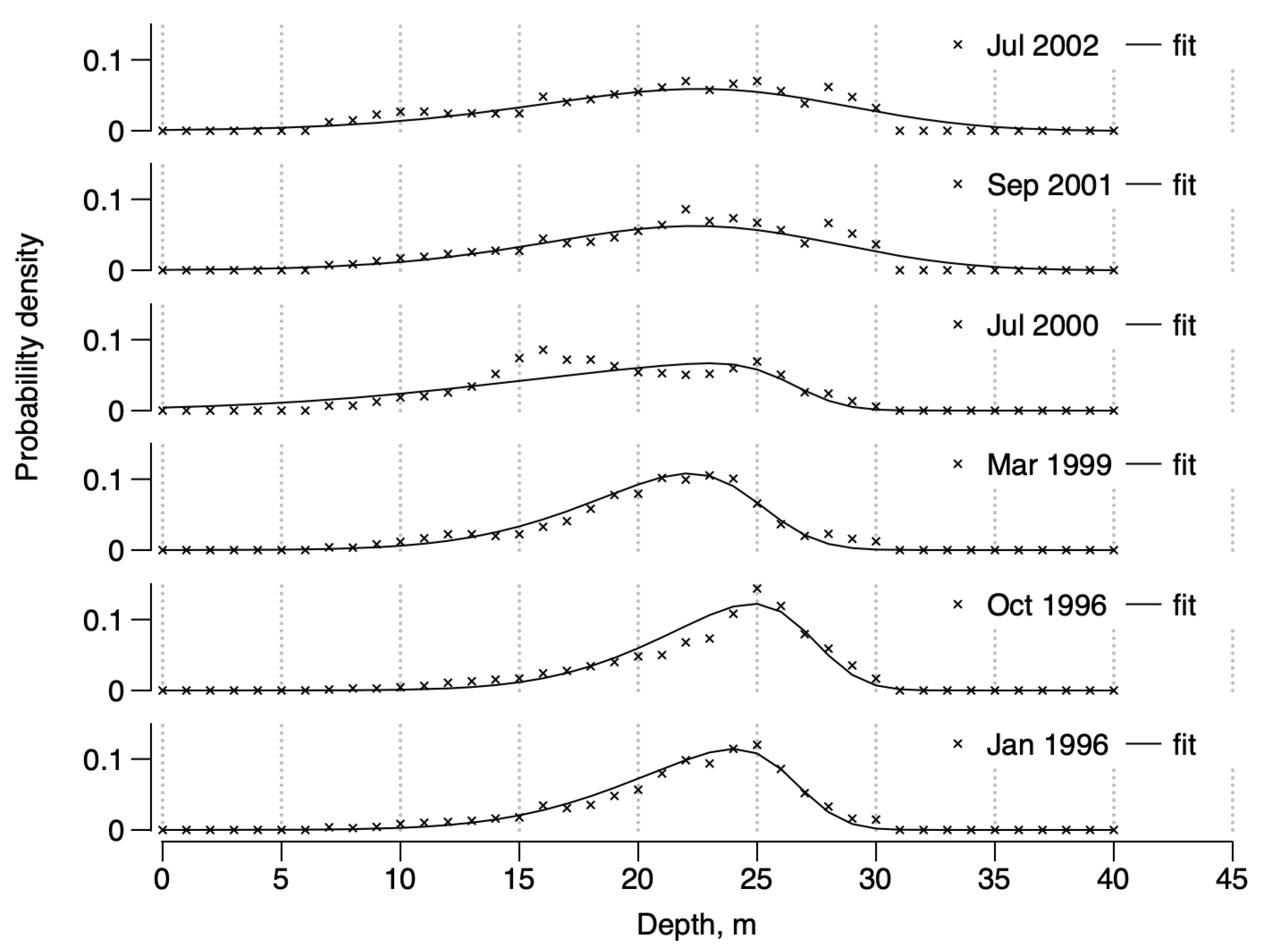
3.1. Spatial Structures of the Population Densities of D. arietina in Banyuls Bay

Empirical semi-variograms were calculated to characterize the spatial distribution structure of the bathymetry and densities (

Table 1. Basic statistics and semi-variogram model fitted to the spatial observations collected at 8 different times on 78 stations, before interpolating the data on a 50 × 50 m grid by kriging. Reported here are the units, number of observation points, minimum values, maximum values, means, variances, the models fitted to the empirical semi-variogram (Gau = Gaussian, Sph = Spherical, Exp = Exponential), the modes (Iso = Isotropic, Ani = Anisotropic), the nuggets $C_0$, the sills $C_0+C_S$, the ranges (in m), and the slopes and ordinates at origin of the cross-validation curve (XV-SLP and XV-OAO).

	z	Jan. 1996	Oct. 1996	Jan. 1998	Mar. 1999	Jul. 2000	Sep. 2001	Jul. 2002	Sep. 2003
Unit	m	$nb.m^{-2}$	$nb.m^{-2}$	$nb.m^{-2}$	$nb.m^{-2}$	$nb.m^{-2}$	$nb.m^{-2}$	$nb.m^{-2}$	$nb.m^{-2}$
Nb pts	76	78	78	78	78	78	78	78	78
Min	4	0	0	0	0	0	0	0	0
Max	32	3550	3000	25	2395	1895	5940	1685	280
Mean	21	491	325	2	174	381	597	245	12
Variance	61	504,245	316,133	17	154,064	271,005	1,200,771	157,037	1665
Model	Gau	Sph	Sph	-	Sph	Sph	Exp	Exp	-
Mode	Ani	Iso	Iso	-	Iso	Iso	Iso	Iso	-
$C_0$	0.1	104,000	100	15	100	1800	1000	100	1611
$C_0+C_S$	121	524,000	314,400	-	135,100	267,900	1,330,000	159,700	-
Range (m)	>1600	524	275	-	308	368	543	549	-
XV-SLP	-	0.925	0.996	-	0.957	1.086	0.893	0.905	-
XV-OAO	-	−12.76	−44.48	-	−36.65	−94.52	−43.95	−18.07	-

). Three models—spheric, exponential, and Gaussian—were fitted to the empirical semi-variogram data. Regarding bathymetry, the best fit was obtained with an anisotropic Gaussian model. The sill of the variogram ($121.00$) is twice the empirical variance ($61.23$) and the effective minimum range exceeds the limit of the active lag distance ($1600m$), with an anisotropic factor equal to ca. 4 on a 90° axis. These results indicate that the changes in bathymetry are very gradual and continuous, oriented, and intrinsically non stationary. Therefore, no kriging was applied and an Inverse Distance Weighted (IDW) interpolation was performed instead.

For population densities, the analysis of two spatial surveys (January 1998 and September 2003) did not permit any structure to be identified, thus no kriging interpolation was performed. Densities were very low and the distribution in both cases was found to be random over the sampling domain (i.e., the semi-variogram is reduced to a pure nugget effect).

For the remaining six surveys in Table 1 there were identifiable structures. In all cases, semi-variograms were isotropic. The calculated sills were close to the empirical variance, assuming that the intrinsic hypothesis of stationarity is respected. In four surveys (January 1996, October 1996, March 1999, and July 2000) the best fits were achieved with a spherical model, suggesting well-identified, dense patches. For two other surveys, in September 2001 and July 2002, the best fits were achieved with an exponential model. This suggests a more continuous structure over the domain sampled. The structures’ maximum range (i.e., the average patch radius) was ca. $550m$. In all cases, the cross-validations were good enough to perform a point ordinary kriging on the observations.

The total number of D. arietina individuals decreased from January 1996 to January 1998, then re-increased from March 1999 to September 2001, before deceasing again until September 2003 (see Table 1, “Means”). The resulting skew-normal frequency distributions of individual densities as a function of depth (z, from Equation (1)) are shown in Figure 4.

Parameter estimates (

Table 2. Parameter estimates of the skew-normal distribution linking averaged densities ($ind.m^{-2}$) to depth z in m, for each of the 8 surveys performed in Banyuls Bay between 1996 and 2003. For two surveys, January 1998 and September 2003, densities were too low and no fitting or distributions could be performed. The three fitted parameters are $\omega$, $\xi$ and $\lambda$; they were used to the calculate mean, variance, skewness, and kurtosis, see Equation (1).

	$\mathit{\omega }$	$\mathit{\xi }$	$\mathit{\lambda }$	Mean	Variance	Skewness	Kurtosis
January 1996	6.02	26.62	−3.77	21.98	14.70	−0.76	0.61
October 1996	5.48	27.32	−3.27	23.14	12.53	−0.71	0.55
January 1998	-	-	-	-	-	-	-
March 1999	6.06	25.04	−2.96	20.46	15.75	−0.66	0.50
July 2000	11.15	26.54	−6.55	17.75	46.96	−0.91	0.77
September 2001	8.21	26.85	−1.31	21.64	40.27	−0.24	0.13
July 2002	9.24	27.65	−1.60	21.40	46.29	−0.33	0.20
September 2003	-	-	-	-	-	-	-

) show that $\omega$ varied between $5.48$ and $11.15$, $\xi$ varied between $25.04$ and $27.65$, and $\lambda$ varied between $-1.31$ and $-6.55$. Hence, all distributions are right-skewed. The means of the distributions varied between $17.75$ and 23.14 m and the variances varied between $12.53$ and $15.75$ before the end of 1999, and between $40.27$ and $46.96$ thereafter, indicating a wider distribution for the depth range concerned (0–40 m). Skewness and kurtosis showed similar trends, being higher in the first part (around $-0.71$ and $0.55$, respectively) than in the second part, after year 2000 (around $-0.28$ and $0.16$, respectively). The only exception in the data series is the year 2000, which had the most pronounced skewness ($-0.91$) and kurtosis ($0.77$) values.

These results imply that, in general, the maximum density is expected at about $26m$ water depth, that the minimum depth at which D. arietina can be observed is $z_{min}=2m$, and that the maximum depth is expected to be $z_{max}=32m$. The variability in maximum values and sizes of the patches indicates, nonetheless, that they do not respond to either a proportional density distribution (sizes will remain approximately constant) or a constant density distribution (maximum values will remain approximately constant), indicating an absence of density regulation processes.

3.2. Demographic Parameters of the D. arietina Population

The parameters of the growth function, the averaged growth rate $\gamma$, and the maximum size $s_{max}$, were estimated from Medernach et al. [14] and Charles et al. [20]. Values of $\gamma$ and $s_{max}$ were, respectively, $0.0035\pm 0.0006$ (SE) $da{y}^{-1}$ and $25\pm 2$ (SE) $mm$. The mortality rate, $\mu$, was estimated from the exponential decrease in the densities during two long periods with no recruitment (June 1994 to November 1996 and November 2001 to June 2004). It was found to be equal to $0.0045\pm 0.0020$ (SE) $da{y}^{-1}$.

The size at reproduction, or maturity, was estimated to be $18\pm 1mm$ [20]. The steady-state estimate of the number of recruits per reproducer, with $\mu =0.0045da{y}^{-1}$ and $T=365days$, is ${\rho }^{★}=4.16$ recruits per reproducer (Figure 5). In other words, with a constant annual recruitment, the population of D. arietina in the Bay of Banyuls-sur-Mer can be maintained at steady state if a reproducer generates, on average, ca. 4 reliable recruits. If they produce more, the total abundance, $N_t$, increases and diverges to infinite (the model does not represent density-dependent limitations). If they produce less, the total abundance, $N_t$, decreases asymptotically to zero (corresponding to the local extinction of the population). The general form of the series is:

$$\left\{\rho =\delta {\rho }^{★},\delta \in \mathbb{R},N_{t+\Delta t}=N_t(\delta +\alpha (1-\delta )\right\}$$

(17)

where $\delta$ (dimensionless) is a multiplier of the number of recruits per reproducer at equilibrium.

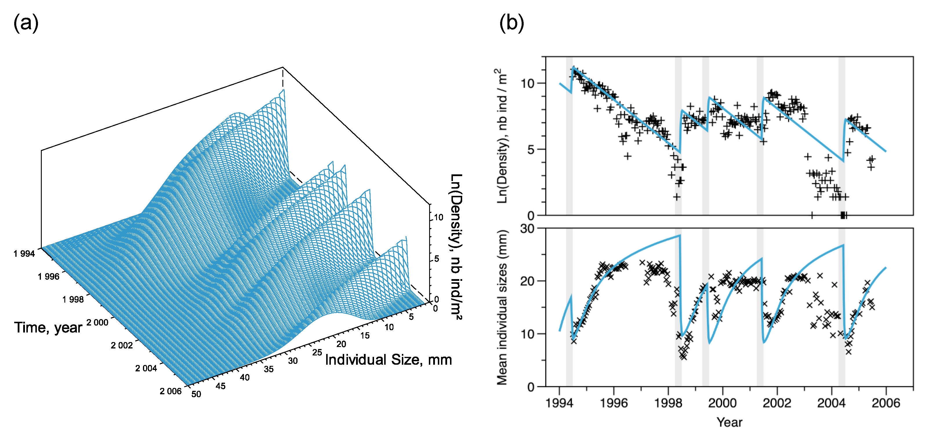
3.3. Simulating the Temporal Variations

The next step was to simulate the dynamics of the D. arietina population in Banyuls Bay, and to compare results with the data series recorded at the long term observation station located in the bay (“SOLA”, Figure 2 and Figure 6). The transition due to the relocation of the SOLA station occurred around day 1000 of the simulation, when the number of individuals in the bay was low. No step effect was detected at this time, but the data series from 1994 to 1996 were re-aligned to fit with the new $27m$ SOLA station where the 1997–2005 data series were collected. This re-alignment was conducted using the spatial surveys, where estimated abundances at the two stations can be resolved simultaneously. This provided an average conversion factor of $3.2$, i.e., the densities at $27m$ were assumed to be about three times the densities at $18m$.

Recruitment events occurred in 1994, 1998, 1999, 2001, and 2004 (Figure 6), with an average period $T=730$ days over the 10 year long observation period. Using Equation (12), the recruitment rate at equilibrium was estimated as ${\rho }^{★}=25.71$ recruits per reproducer (see Figure 5). The initial condition of the simulation, $N\left(0\right)$, that minimised the square distance between observations and simulations was equal to 12,000 $ind.m^{-2}$ with a normal size distribution of $10\pm 2.0$ (SD) $mm$, while filtering a part of the variability, the model simulates correctly the observed pattern of total abundances and the amplitude of recruitment peaks (Figure 6b). Ranges of fluctuations were large; the maximum estimated abundance value was reached in 1994 ($51ind.m^{-2}$). The minimum estimated value was reached in 1998 ($520ind.m^{-2}$); however, the model overestimated densities in 1998 and 2003–2004. It reproduced the averaged length well (Figure 6b) but slightly overestimated the maximum and minimum average lengths. Strong decreases in average animal length indicate when recruitment occurred. It also shows that the period between 2003 and 2004 was an exception with very low densities (as observed in the 2003 spatial survey) but small size individuals, followed by a large peak of recruitment in 2004, returning to a situation of better predictability.

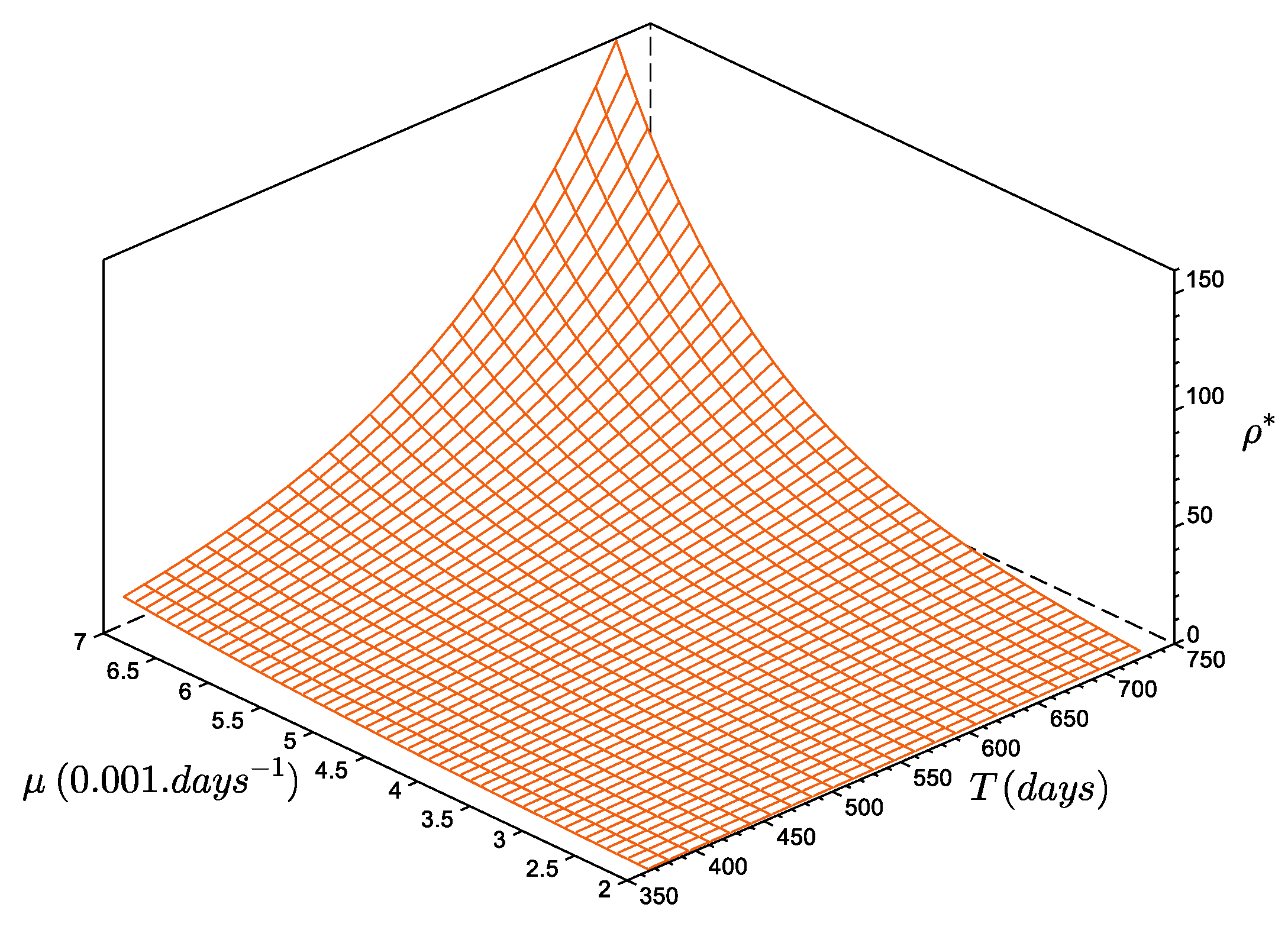
3.4. Extrapolating the Population Dynamics in Time and Space

Population density variations were first calculated over ca. 180 years, using Equation (9) applied to the estimated series of $T_i$ successive periods between two recruitments from 1824 to 2004. The initial condition for all cases was determined for the optimal simulation fitting with the 10-year survey and was equal to $1000ind.m^{-2}$ (Figure 7), corresponding to the value of the last recorded recruitment peak in 2004, and hence where all scenarios are supposed to converge at the end of the simulations.

Three long-term trends were simulated using different averaged versions of the NAOi series (1 year, 6 month, and 3 month averages). The year of maximum population density for each of the three simulations is given on Figure 7a. The simulations indicated that:

• For a yearly-averaged NAOi, the estimate for ${\rho }^{★}$ was $23.56$ recruits per reproducer. This produced a maximum density during 1930, of almost $35.{10}^{6}ind.m^{-2}$; the minimum value occurred during 1881 ($0.012ind.m^{-2}$, or about 72 individuals in the entire bay).
• If the first 6 months of the NAOi are averaged, then the $\rho *$ estimate was slightly lower ($18.43$ recruits per reproducer); this simulation reached its maximum density value in 1928, with fewer individuals: $9500ind.m^{-2}$. The minimum value was reached during 1874 ($0.007ind.m^{-2}$).
• Using a 3 month averaged NAOi (April, May, and June concerned by larval dispersal and recruitment), the highest estimate for ${\rho }^{★}$ was obtained: $47.06$ recruits per reproducer. In this case, the maximum value was reached earlier in 1914, with about $75.{10}^{9}ind.m^{-2}$; the minimum value occurred later, in 1943, i.e., after the maximum peak. This minimum was only $0.001ind.m^{-2}$, and is lower than the other two cases.

Figure 7b highlights the simulation trends corresponding to the interval when observations were made in Banyuls Bay. The simulated recruitment event in 2000 (marked in orange on Figure 7b) was not observed in the field observations (marked in blue, Figure 7b). Indeed, none of the simulations replicated the 2001 event observed. The 6 month averaged NAOi simulation predicted eight recruitment events (1994, 1995, 1998, 1999, 2000, 2002, 2003, and 2004). The last case (3 month NAOi average) predicted only four recruitment events during: 1994, 1999, 2002, and 2004.

Figure 7c,d illustrate the variations in the averaged sizes of individuals in the population. Even if simulations are not synchronous with each other, the variations are in the same ranges for all three cases. Within the time frame of the observations from Banyuls Bay, the simulation corresponding to the yearly-averaged NAOi is closest to the observations, even if it tended to overestimate values, mostly prior to actual recruitment events.

Using the metapopulation model, estimates of the sub-population densities of D. arietina in the metapopulation (Figure 8) were made at the regional scale of the Gulf of Lions. The region was divided in 21 transects, each considered as a sub-population. Simulations were performed using the 10-year series of expected recruitment in the region as it was observed in Banyuls Bay (Figure 6) until a steady state was reached (a minimum of five cycles were required to achieve equilibrium).

Steady-state estimates of densities in 1998 (post-recruitment) were compared with the averaged measured densities for each local population. All simulations use Equations (12) and (14) in both their closed and open system configurations; parameter values were identical to those used to simulate the data series collected in Banyuls Bay. The recruitment rates were chosen to be equal to the estimate at steady-state (${\rho }^{★}=25.71$).

In a closed system, because of the east-to-west circulation in the Gulf of Lions, there is a progressive accumulation of individuals from Transect 21 to 1. However, for an open system, with a flux of recruits entering at Transect 21 at a rate equal to the recruitment rate, the model reproduces quite well the observed distribution pattern (Figure 8). In particular, the series of peaks around transects 4, 10, and 17 (Figure 8b). No samples from Transect 19 had D. arietina individuals, while all simulations suggested it would be present.

4. Discussion

In this study, we explored how well the population dynamics of a species exhibiting strong abundance fluctuations would be represented by a minimal model without any regulation processes. The challenge was to build a model that could represent the dynamics of population irruptions realistically, at both a local scale (<${10}^{1}k{m}^2$) and a larger, regional scale of the metapopulation (>${10}^{3}k{m}^2$), even when few data are available. Our model mixes continuous dynamics with discrete outbreaks events without any limitation factors; this is a departure from earlier work representing the dynamics of the same species using a discrete metapopulation model with a limitation function [17].

4.1. Mathematical Properties of the Population Outbreak Models

The mathematical properties of our model were studied to demonstrate the existence of a macroscopic, positive equilibrium in the dynamics of the system. This is not trivial since the continuous model (Equation (3)) by itself would lead to extinction of D. arietina, while the discrete recruitment events monotonously and exponentially increase the population size.

The combination of continuous and discrete processes demonstrated that on long timescales and over large areas (Equation (13)), whatever the series or sequence of intervals between two consecutive recruitments are, will lead to an equilibrium as long as either:

• ${\rho }^{★}$ is fixed (Equations (10), (11) and (15)); or
• The system is controlled by an external flux of individuals from outside of the study area (Equation (16)).

The species outbreak is in a local transitory phase because it is followed by a sharp decrease in the population. But, the possibility to reach a macroscopic steady-state suggests that a pool of individuals can be maintained to create new outbreak events when conditions are fulfilled.

These mathematical properties are sufficient in our modelling study to describe the plausible dynamics of a species outbreak as it was observed and without any limitation factors. However, some simulated density values in long term simulations were estimated as too high, suggesting that in real systems, potential regulatory processes could be expressed to limit exponential increases. In the data series at our disposal such a limitation could not be identified, and consequently, cannot be accounted for.

4.2. Characteristics of the Local Population Dynamics

The large density variability, the absence of regulation mechanisms, including the apparent lack of competition with other species [1] and the absence of a pattern of proportional or constant density distributions justified that the species be qualified as an “outbreak” species [2] (Figure 4). It may also be characterised as dynamically independent from other species in the benthic community. Furthermore, the model of local population dynamics in Banyuls Bay does not imply that the population is isolated. Instead it shows that the balance is null between emigration and immigration of individuals at the larval stage before recruitment. In other words, the quantity of recruits, attributed solely to local individuals, can also arrive from outside the bay as long as local individuals are exported in the same quantity of recruits.

The primary model built to simulate the dynamic of the D. arietina population (Continuous model, Section 2.2.1) did not contain any limitation function, either by food or space resources. This model represents changes in the size distribution of individuals. In these dynamics, the crucial parameter is the size at which juveniles become reproducing adults ($s_{rep}=18$ $mm$ [20]). A direct comparison with the size structure distribution observed at the SOLA station was not possible because: (i) the variability has two components, spatial and temporal, and (ii) the parameters of growth, mortality and recruitment were not known a priori and were rebuilt using relationships published in Merdernach et al. [14]. Instead, a comparison between simulations and observations were made using an independent data series of mean individual weights (Figure 6b).

Although D. arietina is not a well-documented species, its demographic characteristics suggest that it is a pioneer species with a strong ability to colonize suitable habitats [37]. The population of D. arietina is composed of small size organisms (the average maximum size is ca. $30mm$) and a fast growth rate (maximum size is reached in ca. 1 year), and a short lifespan (2 years) [1,14]. With 9000 eggs per female on average, the fecundity is moderately high for a polychaete species [37]. The absence of regulation suggests that neither growth not mortality rates appear to be influenced by changes in environmental conditions (regulating the presence or absence of recruitment) or by the state of the population itself (low vs. high abundances). No seasonal trend was detected and the survival curves were identified between two recruitment events as decreasing exponential functions with a constant mortality rate.

The parameter ${\rho }^{★}$, which is the number of recruits per reproducer, is a steady-state estimated value interpreted in terms of demography, as a function of the mortality rate and the duration between two recruitment events (Figure 5). Values of ${\rho }^{★}$ are very small compared to the average number of eggs produced per female [20,37], even for a 3-year period of no recruitment (${\rho }^{★}=137$). This characteristic combined with an absence of regulation means the species has a high potential for proliferation: when $\rho$ is greater than ${\rho }^{★}$, the average biomass increases exponentially. Such a proliferation usually induces a density-dependent process of recruitment [38], but this was not observed during the 10-year survey, and the recruitment event of 1994, which had the highest density values, does not provide any information on potential limitations.

A large part of the inter-annual variability in population abundance was assumed to be from variations in the recruitment success (i.e., settlement of juveniles at size $s_0=1$ $mm$). This is a common property of sedentary benthic marine invertebrates, having a pelagic larval dispersion phase [39,40]. Several factors may influence the recruitment success: the larval and post-larval mortality, physical disturbance of the habitat, and competition for resources. The larval and post-larval mortality due to predation is probably one of the factors controlling recruitment here [41,42,43]. Larvae may even be consumed by adults of the same species as they filter particles in the water column without active sorting [44]. In addition, Banyuls Bay is open, subject to hydrodynamic forces that increase during storms, inducing stress at the sediment surface, and possibly preventing recruitment events [16]. Intensity and frequency of storms were therefore assumed to explain a large part of the success or the failure of the recruitment. In this situation, a storm may have two effects: (i) to increase the larval dispersion [22] and (ii) to increase mortality of juveniles that just settled. Even if some population dynamic models take into account explicitly larval and post-larval mortality [41,45], we have chosen not to do so because the sensitivity of recruitment to a small perturbation is high and could have generated larger discrepancies between observations and simulations, due to propagation of the uncertainties [40].

4.3. Influence of the NAO on Recruitment

For the local population simulation, the occurrence of recruitment events was assessed from field observations. For longer-term simulations (>10 years), it was necessary to use a proxy for recruitment, since no long time series are available and historical observations are very rare [23]. The NAO index was selected as an indirect proxy for recruitment [46] because it is a reliable indicator of the winter storms regime on the European continent [34,47]. Storms are deviated to the north when NAOi is positive, and south, over the Mediterranean basin, when the index is negative. This pattern has consequences on the ocean physics [48], and on marine systems [49].

Monthly NAOi values were averaged over different time intervals (3, 6, and 12 months) which could be considered relevant to the recruitment process [49]. Results showed that the choice of the time window over which the NAO index is averaged conditions the pattern of density variations. Comparing the last values of the simulations with data collected in Banyuls Bay, and without any other constraint than all simulations must match with the last observed peak in 2004, it was concluded that the use of the yearly averaged NAOi provided the best fit with the ten-year series. The second best fit was obtained with simulations using the 3-month averaged NAOi. Conversely, simulations using the first 6-months averaged NAOi, did not provide a good match (it generated three unobserved recruitment events).

In all extrapolations, the minimum values reached were very low, but without leading to local exclusion. Using the 3-month averaged NAOi simulated unrealistically high maximum values. To a lesser extent, this is also true of the yearly averaged NAOi. When no mechanisms of regulation are accounted for, densities are expected to fluctuate between extremes over long time simulations. Using the NAOi, the average size of all individuals fluctuated within ranges comparable to those observed in Banyuls Bay; nonetheless, all the simulations tended to overestimate the minimum and maximum observed values.

The choice of a climate index to simulate recruitment dynamics in the Mediterranean basin is not limited to the NAO [50]. There are other indices, like the Mediterranean Oscillation (MO) indices (e.g., the Western MO [51,52]) which is also suitable for the simulations. However, the NAO and MO indices are correlated [51] and changing for a regional index would not be expected to improve these simulations, but only to add more variability. Climate indices will always match imperfectly with recruitment patterns and can only be used as probabilistic estimators of recruitment occurrence [52].

4.4. Is the Population of D. arietina a Metapopulation?

Ecologically, a successful recruitment is favoured by a successful larval development [53], and during the dispersion phase (which may vary from days to months) larvae of marine invertebrates are transported passively by currents. Larvae can also choose their substratum. For example, Capitella sp. [54] prefers to colonize fine, muddy sediments enriched with organic matter, and Spisula solidissima and Mulinia lateralis inhabit coarse sand sediments preferentially [43,55]. In our case, juveniles of D. arietina build a tube made of mucus first [20], and were not observed to colonize muddy sediments, which are unfavourable for their development. However, no process of sediment selection occurs [20], and there are no unique criteria that explain the spatial distribution, even if it is partly related to depth and sediment characteristics. This lack of strong deterministic factors conditioning recruitment and the stochastic nature of the processes governing outbreak dynamics has been characterised on long time scales in continental ecology. For example, Régnière and Nealis [56] emphasised the importance of considering outbreaks in spatially distributed sites because of the difficulty to predict outbreaks based on the variability of the local recruitment.

The long-term temporal simulations of local dynamics can lead to a macroscopic stability, despite strong variations in event occurrences. This suggests that the population persistence is ensured on long time scales, even if the intervals between two recruitment events fluctuate in duration. However, calling this local dynamics does not imply the population is isolated. The recruitment rate at macroscopic equilibrium, ${\rho }^{★}$, is a constraining term which encompasses implicitly not only a balance between local recruitment and mortality, but also between the emigration and immigration of larvae.

The use of a metapopulation framework makes explicit this notion of macroscopic stability for the case of an open system. It is an extension of the local hybrid formulation adding spatial components to the local demographic processes, and leads to reformulate analytically the macroscopic steady state without to condition its existence to a single, particular fixed value of a recruitment rate at equilibrium: ${\rho }^{★}$. Therefore, an unconstrained recruitment rate $\rho$, together with the other parameters ensures the global equilibrium. By taking into account explicitly spatial processes in an open metapopulation system, this relaxes the steady-state condition imposed by using a single recruitment rate. Thus, it is the calculations performed within a larger metapopulation framework defined at the regional scale of the Gulf of Lions (Figure 8), that explicitly shows the spatial dynamics. In the specific configuration of the D. arietina metapopulation, structured by spatial exchanges oriented globally from northeast to southwest, the results show that a closed metapopulation did not make any sense; the individuals progressively accumulated to the Southwestern part of the domain, without exhibiting strong oscillations, even with a variable duration between recruitment events. Only the open-metapopulation case presents interesting outcomes; it shows not only that it is possible to reach a steady-state consistent with the observed pattern, but also that the oscillation pattern changes with time (in intensity and location), when applying a varying duration between two recruitment events. Direct optimisation of the simulations with the observations is of little use here because there was insufficient information on recruitment events in the local system. Furthermore, only one data set was available that did not overlap with the Banyuls Bay surveys [24]. The best possible hypothesis was to consider that it reflected a steady-state situation.

4.5. Implications of the Modelling

The model framework discussed in this article investigates mechanisms that explain a seemingly stochastic demographic variability as observed in real ecological systems, and which are characterised as outbreak dynamics. The most prominent feature of outbreak species dynamics is the absence of regulation. However, it is worth noting that outbreak dynamics are not a common feature for benthic systems where substrate surface area limitations usually apply. Indeed, the most common regulation factors are density-dependence [57,58] or self-organization [59], both requiring different formulations to be accounted for.

In the past, even if marine species outbreaks have not attracted a lot of attention compared to their terrestrial counterparts, some marine population changes have been reported as outbreaks, mainly because of their negative effects on societies. A classic example of this is the history of the shipworm (Teredinidae) in 18th century Europe and the subsequent political fallout it caused [60]. Ironically, shipworms cannot be classified as an outbreak species, a priori, because this taxa has a strong regulating factor, which is its density dependence on a wood substrate [61,62]. Hence, as soon as the substrate supply disappears (e.g., wooden harbour infrastructure and boat hulls) shipworm infestations slow and cease to be of concern.

Our modelling framework therefore emphasised the main characteristics of an outbreak species: the absence of sensitivity to regulating factor(s). A minimal formulation was used to simulate outbreak population dynamics with discrete recruitment periods [63]. Implementing a mechanistic approach permitted exploration of the dynamics of outbreaks based on interactions between continuous and discrete processes. In the case of the species studied here (D. arietina), the model shows that population irruptions can be described accurately with a minimal set of processes and can exhibit macroscopic stability over long time periods and large areas, without imposing any limitations (resources, density dependence, predation, etc.). The framework presented is comprehensive, and may be suitable for other marine species exhibiting population outbreaks.

Intriguingly, the plausible absence of unexpressed population regulation factors was not an issue either for the long-term or regional scale extrapolations. In other words, the situation observed at one moment, or at one place, cannot be interpreted as a consequence of either a past, or spatially distant process(es) that influence the population size. Unfortunately this also means that trying to fill in data gaps from historical, anecdotal sources is unlikely to provide information necessary for reconstructing past outbreaks because of the fragmentary, partial nature of recovered data [64] and validation challenges [65]. Paradoxically in this case, while hindcasting past fluctuations is possible, we are unlikely to uncover historical material evidence of outbreak events because the species itself has not elicited any widespread interest.

Our results also have an important implication for inclusion of outbreak species in benthic water quality indices. There are a number of studies on D. arietina that have focused on detecting statistical correlations between benthic community indices and environmental changes (e.g., [12,18,24,25,26], and references therein). The results indicate that the use of D. arietina in the calculation of benthic indices is not recommended. Environmental quality indices assume that environmental conditions act as a regulating factor on the included species, which is a false assumption for outbreak species. For D. arietina, in particular, this has already generated confusing and contradictory interpretations of different indices (see discussion in [12]).

Lastly, we noticed several knowledge gaps. During the study, it became apparent that the determinism of the recruitment step is not fully understood and that the recruitment process may even be more stochastic than deterministic. It would be desirable to improve the metapopulation boundary definition with population genetics information (e.g., [65,66]). In addition, recruitment processes controlled by integrative climate indices alone will not be accurate enough to comprehensively determine the dynamics of outbreak species without ancillary studies. Thus, systematic tests against multiple climatic indices are suggested to explain recruitment variability, even if the quest for the perfect index is illusory. Nonetheless, while our results showed that local variability is explained adequately by the NAOi, it is important to acknowledge that the simulations could not have been evaluated without the earlier comprehensive, multi-year demographic studies accomplished in Banyuls Bay. These types of surveys remain too rare because they are labour intensive and costly, yet they provide crucial information about size distributions required by population dynamics theory.

In general, even if the macroscopic steady-states are known, the predictability of the system is not guaranteed. Predictability is based on ensuring that the processes included are robust and that state variable estimates are precise. However, ecology is a lawless science [67] because a single system can be described by many possible formulations at different levels of organisation and each of them has their own sets of advantages and disadvantages [68]. But, all of them have a low final predictability. One way around this would be to implement formal forecasting methods [69]. This can be achieved using advanced data assimilation or optimal control techniques in a formalised, quantitative reasoning framework linking physiological and environmental parameters (e.g., [70,71]). This, however, requires access to long, continuous data series, including for the environmental variables hypothesised to influence the outbreaks.

5. Conclusions

This study is seen as a new starting point to improving the quantification of a species’ outbreak episodes. The model is designed to explore how marine invertebrates that have the characteristics of an outbreak species persist in their environment despite very large local fluctuations and an apparent lack of regulation mechanisms. In contrast with the majority of outbreak species models, we have explicitly formulated outbreaks as discrete processes within continuous dynamics as a hybrid dynamic model. The model’s mathematical properties were characterised in time and space to identify equilibrium conditions, which demonstrated that even if D. arietina disappears from a particular locality for a period, the population will be maintained at the larger scale of the metapopulation. This leads us to conclude that marine species outbreaks would be best studied at the relevant regional scale, not local scales, together with comprehensive demographic studies of the species in question.

References

1. Gremare, A.; Sarda, R.; Medernach, L.; Pinedo, S.; Amouroux, J.M.; Martin, D.; Nozais, C.; Charles, F. On the dramatic increase of Ditrupa arietina O.F. Müller (Annelida: Polychaeta) along both the French and the Spanish Catalan coasts. Estuarine Coast. Shelf Sci. 1998, 47, 447–457. [Google Scholar] [CrossRef]
2. Hanski, I. Density dependence, regulation and variability in animal populations. Philos. Trans. Biol. Sci. 1990, 330, 141–150. [Google Scholar] [CrossRef]
3. Condon, R.H.; Duarte, C.M.; Pitt, K.A.; Robinson, K.L.; Lucas, C.H.; Sutherland, K.R.; Mianzan, H.W.; Bogeberg, M.; Purcell, J.E.; Decker, M.B.; et al. Recurrent jellyfish blooms are a consequence of global oscillations. Proc. Natl. Acad. Sci. USA 2013, 110, 1000–1005. [Google Scholar] [CrossRef]
4. Uthicke, S.; Schaffelke, F.; Byrne, M. A boom-bust phylum? Ecological and evolutionary consequences of density variations in echinoderms. Ecol. Monogr. 2009, 79, 3–24. [Google Scholar] [CrossRef]
5. Harris, L.G.; Gibson, J.L. Contrasting decadal recruitment patterns in the sea urchin Strongylocentrotus droebachiensis in the Gulf of Maine. J. Exp. Mar. Biol. Ecol. 2023, 558, 151832. [Google Scholar] [CrossRef]
6. Pratchett, M.S.; Caballes, C.F.; Cvitanovic, C.; Raymundo, M.L.; Babcock, R.C.; Bonin, M.C.; Bozec, Y.M.; Burn, D.; Byrne, M.; Castro-Sanguino, C.; et al. Knowledge Gaps in the Biology, Ecology, and Management of the Pacific Crown-of-Thorns Sea Star Acanthaster sp. on Australia’s Great Barrier Reef. Biol. Bull. 2021, 241, 330–346. [Google Scholar] [CrossRef] [PubMed]
7. Guarini, J.M.; Sari, N.; Moritz, C. Modelling the dynamics of the microalgal biomass in semi-enclosed shallow-water ecosystems. Ecol. Model. 2008, 211, 267–278. [Google Scholar] [CrossRef]
8. Hartley, J.P. A review of the occurrence and ecology of dense populations of Ditrupa arietina (Polychaeta: Serpulidae). Mem. Mus. Vic. 2014, 71, 85–95. [Google Scholar] [CrossRef]
9. Buhl-Mortensen, L.; Ellingsen, K.E.; Buhl-Mortensen, P.; Skaar, K.L.; Gonzalez-Mirelis, G. Trawling disturbance on megabenthos and sediment in the Barents Sea: Chronic effects on density, diversity, and composition. ICES J. Mar. Sci. 2016, 73, 98–114. [Google Scholar] [CrossRef]
10. OBIS. Distribution Records of Ditrupa arietina (O. F. Müller, 1776); Ocean Biodiversity Information System; Intergovernmental Oceanographic Commission of UNESCO: Ostend, Belgium, 2023. [Google Scholar]
11. Resgalla, C.J.; Petri, L.; da Silva, B.G.T.; Brilha, R.T.; Araujo, T.C.; Almeida, M. Outbreaks, coexistence, and life cycle of jellyfish species in relation to abiotic and biological factors along a South American coast. Hydrobiologia 2019, 839, 87–102. [Google Scholar] [CrossRef]
12. Labrune, C.; Amouroux, J.M.; Sarda, R.; Dutrieux, E.; Thorin, S.; Rosenberg, R.; Gremare, A. Characterization of the ecological quality of the coastal Gulf of Lions (NW Mediterranean). A comparative approach based on three biotic indices. Mar. Pollut. Bull. 2006, 52, 34–47. [Google Scholar] [CrossRef]
13. Muxika, I.; Borja, A.; Bonne, W. The suitability of the marine biotic index (AMBI) to new impact sources along European coasts. Ecol. Indic. 2005, 5, 19–31. [Google Scholar] [CrossRef]
14. Medernach, L.; Jordana, E.; Gremare, A.; Nozais, C.; Charles, F.; Amouroux, J.M. Population dynamics, secondary production and calcification in a Mediterranean population of Ditrupa arietina (Annelida: Polychaeta). Mar. Ecol. Prog. Ser. 2000, 199, 171–184. [Google Scholar] [CrossRef]
15. Kritzer, J.P.; Sale, P.F. Metapopulation ecology in the sea: From Levins’ model to marine ecology and fisheries science. Fish Fish. 2004, 5, 131–140. [Google Scholar] [CrossRef]
16. Guizien, K.; Charles, F.; Hurther, D.; Michallet, H. Spatial redistribution of Ditrupa arietina (soft bottom Mediterranean epifauna) during a moderate swell event. Cont. Shelf Res. 2010, 30, 239–251. [Google Scholar] [CrossRef]
17. Guizien, K.; Bramanti, L. Modelling ecological complexity for marine species conservation: The effect of variable connectivity on species spatial distribution and age-structure. Theor. Biol. Forum 2014, 107, 47–56. [Google Scholar]
18. Labrune, C.; Gremare, A.; Amouroux, J.M.; Sarda, R.; Gil, J.; Taboada, S. Assessment of soft-bottom polychaete assemblages in the Gulf of Lions (NW Mediterranean) based on a mesoscale survey. Estuar. Coast. Shelf Sci. 2007, 71, 133–147. [Google Scholar] [CrossRef]
19. Koehler, R. Résultats Scientifiques de la Campagne du “Caudan” Dans le Golfe de Gascogne, Août-Septembre 1895 (1896); Fascicule 26 in Annales de l’Université de Lyon, Masson et Cie: Paris, France, 1896; p. 740. [Google Scholar]
20. Charles, F.; Jordana, E.; Amouroux, J.M.; Gremare, A.; Desmalades, M.; Zudaire, L. Reproduction, recruitment and larval metamorphosis in the serpulid polychaete Ditrupa arietina (O.F. Müller). Estuar. Coast. Shelf Sci. 2003, 57, 435–443. [Google Scholar] [CrossRef]
21. Jordana, E.; Gremare, A.; Lantoine, F.; Courties, C.; Charles, F.; Amouroux, J.M.; Vétion, G. Seasonal changes in the grazing of coastal picoplankton by the suspension-feeding polychaete Ditrupa arietina O.F. Müller). J. Sea Res. 2001, 46, 245–259. [Google Scholar] [CrossRef]
22. Guizien, K.; Brochier, T.; Duchêne, J.C.; Koth, B.S.; Marsaleix, P. Dispersal of Owenia fusiformis larvae by wind-driven currents: Turbulence, swimming behaviour and mortality in a three dimensional stochastic model. Mar. Ecol. Prog. Ser. 2006, 311, 47–66. [Google Scholar] [CrossRef]
23. Gremare, A.; Amouroux, J.M.; Vetion, G. Long-term comparison of macrobenthos within the soft bottoms of the Bay of Banyuls-sur-mer (Northwestern Mediterranean Sea). J. Sea Res. 1998, 40, 281–302. [Google Scholar] [CrossRef]
24. Labrune, C.; Grémare, A.; Guizien, K.; Amouroux, J.M. Long-term comparison of soft bottom macrobenthos in the Bay of Banyuls-sur-Mer (North-Western Mediterranean Sea): A reappraisal. J. Sea Res. 2007, 58, 125–143. [Google Scholar] [CrossRef]
25. Bonifácio, P.; Grémare, A.; Gauthier, O.; Romero-Ramirez, A.; Bichon, S.; Amouroux, J.M.; Labrune, C. Long-term (1998 vs. 2010) large-scale comparison of soft-bottom benthic macrofauna composition in the Gulf of Lions, NW Mediterranean Sea. J. Sea Res. 2018, 131, 32–45. [Google Scholar] [CrossRef]
26. Bonifacio, P.; Grémare, A.; Amouroux, J.M.; Labrune, C. Climate-driven changes in macrobenthic communities in the Mediterranean Sea: A 10-year study in the Bay of Banyuls-sur- Mer. Ecol. Evol. 2019, 9, 10483–10498. [Google Scholar] [CrossRef]
27. Moritz, C.; Loeuille, N.; Guarini, J.M.; Guizien, K. Quantifying the dynamics of marine invertebrate metacommunities: What processes can maintain high diversity with low densities in the Mediterranean Sea? Ecol. Model. 2009, 220, 3021–3032. [Google Scholar] [CrossRef]
28. Guille, A. Bionomie benthique du plateau continental de la côte catalane française IV. Densités, biomasses, et variations saisonnières de la macrofaune. Vie Milieu 1971, 22, 93–158. [Google Scholar]
29. Gupta, A.K.; T, C. Goodness-of-fit tests for the skew-normal distribution. Commun.-Stat.–Simul. Comput. 2001, 30, 907–930. [Google Scholar] [CrossRef]
30. Gros, P. Prévision à moyen terme des fluctuations des ressources halieutiques: Modèles tautologiques ou autoregenerants ? Ann. L’institut Océanogr. 1992, 68, 211–225. [Google Scholar]
31. Hirsch, C. Numerical Computation of Internal and External Flows. Fundamentals of Numerical Discretization; Wiley Series in Numerical Methods in Engineering; John Wiley and Sons: Hoboken, NJ, USA, 1989; p. 515. [Google Scholar]
32. Jones, P.D.; Jónsson, T.; Wheeler, D. Extension to the North Atlantic Oscillation using early instrumental pressure observations from Gibraltar and South-West Iceland. Int. J. Climatol. 1997, 17, 1433–1450. [Google Scholar] [CrossRef]
33. Climate Research Unit. North Atlantic Oscillation (NAO); University of East Anglia: Norwich, UK, 2017. [Google Scholar]
34. Kutzbach, J.E. Large-scale features of monthly mean northern hemisphere anomaly maps of sea-level pressure. Mon. Weather. Rev. 1970, 98, 708–716. [Google Scholar] [CrossRef]
35. Hurrell, J.W. Decadal trends in the North Atlantic Oscillation and relationships to regional temperature and precipitation. Science 1995, 269, 676–679. [Google Scholar] [CrossRef]
36. Chesson, P.; Lee, C.T. Families of discrete kernels for modeling dispersal. Theor. Popul. Biol. 2005, 67, 241–256. [Google Scholar] [CrossRef]
37. McHugh, D.; Fong, P.P. Do life history traits account for diversity of polychaete annelids? Invertebr. Biol. 2002, 121, 325–338. [Google Scholar] [CrossRef]
38. Marshall, D.J.; Keough, M.J. Effects of settler size and density on early post-settlement survival of Ciona intestinalis in the field. Mar. Ecol. Prog. Ser. 2003, 259, 139–144. [Google Scholar] [CrossRef]
39. Botsford, L.W. Physical influences on recruitment to Californa current invertebrate populations on multiple scales. ICES J. Mar. Sci. 2001, 58, 1081–1091. [Google Scholar] [CrossRef]
40. Ripley, B.J.; Caswell, H. Recruitment variability and stochastic population growth of the soft-shell clam, Mya arenaria. Ecol. Model. 2006, 193, 517–530. [Google Scholar] [CrossRef]
41. Dekshenieks, M.M.; Hofmann, E.E.; Klinck, J.M.; Powell, E.N. A modelling study of the effects of size and depth-dependent predation on larval survival. J. Plankton Res. 1997, 19, 1583–1598. [Google Scholar] [CrossRef]
42. Hiddink, J.G.; Hofstede, R.; Wolff, W.J. Predation of intertidal infauna on juveniles of the bivalve Macoma balthica. J. Sea Res. 2002, 47, 141–159. [Google Scholar] [CrossRef]
43. Weissberger, E.J.; Grassle, J.P. Settlement, first year growth, and mortality of surf clams Spisula solidissima. Estuar. Coast. Shelf Sci. 2003, 56, 669–684. [Google Scholar] [CrossRef]
44. Takasuka, A.; Oozeki, Y.; Kimura, R.; Kubota, H.; Aoki, I. Growth selective predation hypothesis revisited for larval anchovy in offshore waters: Cannibalism by juveniles versus predation by skipjack tunas. Mar. Ecol. Prog. Ser. 2004, 278, 297–302. [Google Scholar] [CrossRef]
45. Ellien, C.; Thiebaut, E.; Barnay, S.; Dauvin, J.C.; Gentil, F.; Salomon, J.C. The influence of variability in larval dispersal on the dynamics of a metapopulation in the eastern Channel. Oceanol. Acta 2004, 23, 423–442. [Google Scholar] [CrossRef]
46. Broitman, B.R.; Mieszkowska, N.; Helmuth, B.; Blanchette, C.A. Climate and recruitment of rocky shore intertidal invertebrates in the eastern North Atlantic. Ecology 2008, 89, S81–S90. [Google Scholar] [CrossRef]
47. Hurrell, J.W.; Kushnir, Y.; Ottersen, G.; Visbeck, M. An Overview of the North Atlantic Oscillation. In The North Atlantic Oscillation: Climatic Significance and Environmental Impact; Hurrell, J.W., Kushnir, Y., Ottersen, G., Visbeck, M., Eds.; Geophysical Monograph Series; American Geophysical Union: Washington, DC, USA, 2003; pp. 1–35. [Google Scholar] [CrossRef]
48. Visbeck, M.; Chassignet, E.P.; Curry, R.G.; Delworth, T.L.; Dickson, R.R.; Krahmann, G. The Ocean’s Response to North Atlantic Oscillation Variability. In The North Atlantic Oscillation: Climatic Significance and Environmental Impact; Hurrell, J.W., Kushnir, Y., Ottersen, G., Visbeck, M., Eds.; Geophysical Monograph Series; American Geophysical Union: Washington, DC, USA, 2003; pp. 113–145. [Google Scholar] [CrossRef]
49. Drinkwater, K.F.; Belgrano, A.; Borja, A.; Conversi, A.; Edwards, M.; Greene, C.H.; Ottersen, G.; Pershing, A.J.; Walker, H. The Response of Marine Ecosystems to Climate Variability Associated with the North Atlantic Oscillation. In The North Atlantic Oscillation: Climatic Significance and Environmental Impact; Hurrell, J.W., Kushnir, Y., Ottersen, G., Visbeck, M., Eds.; Geophysical Monograph Series; American Geophysical Union: Washington, DC, USA, 2003; pp. 211–234. [Google Scholar] [CrossRef]
50. Criado-Aldeneuva, F.; Soto-Navarro, J. Climatic Indices over the Mediterranean Sea: A Review. Appl. Sci. 2020, 10, 5790. [Google Scholar] [CrossRef]
51. Martin-Vide, J.; Lopez-Bustins, J.A. The Western Mediterranean Oscillation and rainfall in the Iberian Peninsula. Int. J. Climatol. 2006, 26, 1455–1475. [Google Scholar] [CrossRef]
52. Lopez-Bustins, J.A.; Arbiol-Roca, L.; Martin-Vide, J.; Barrera-Escoda, A.; Prohom, M. Intra-annual variability of the Western Mediterranean Oscillation (WeMO) and occurrence of extreme torrential precipitation in Catalonia (NE Iberia). Nat. Hazards Earth Syst. Sci. 2020, 20, 2483–2501. [Google Scholar] [CrossRef]
53. Perkins, P.J.; Daniel, K. Variation in larval growth can predict the recruitment of a temperate, seagrass-associated fish. Oecologia 2006, 147, 641–649. [Google Scholar] [CrossRef]
54. Grassle, J.P.; Butman, C.; Mills, S. Active habitat selection by Capitella sp. I Larvae II. Multiple choice experiments in still water and flume flows. J. Mar. Res. 1992, 50, 717–743. [Google Scholar] [CrossRef]
55. Snelgrove, P.V.R.; Butman, C.A.; Grassle, J.P. Hydrodynamic enhancement of larval settlement in the bivalve Mulinia lateralis (Say) and the polychaete Capitella sp. I. in microdepositional environments. J. Exp. Mar. Biol. Ecol. 1993, 168, 71–109. [Google Scholar] [CrossRef]
56. Régnière, J.; Nealis, V.G. Ecological mechanisms of population change during outbreaks of the spruce budworm. Ecol. Entomol. 2007, 32, 461–477. [Google Scholar] [CrossRef]
57. Clare, D.S.; Spencer, M.; Robinson, L.A.; Frid, C.L.J. Species densities, biological interactions and benthic ecosystem functioning: An in situ experiment. Mar. Ecol. Prog. Ser. 2016, 547, 149–161. [Google Scholar] [CrossRef]
58. Savage, A.A. Density dependent and density independent relationships during a twenty-seven year study of the population dynamics of the benthic macroinvertebrate community of a chemically unstable lake. Hydrobiologia 1996, 335, 115–131. [Google Scholar] [CrossRef]
59. Weerman, E.J.; van de Koppel, J.; Eppinga, M.B.; Montserrat, F.; Liu, Q.X.; Herman, P.M.J. Spatial self-organization on intertidal mudflats through biophysical stress divergence. Am. Nat. 2010, 176, E15–E32. [Google Scholar] [CrossRef] [PubMed]
60. Serruys, M.W. The Societal Effects of the Eighteenth Century Shipworm Epidemic in the Austrian Netherlands (c. 1730–1760). J. Hist. Environ. Soc. 2022, 6, 95–127. [Google Scholar] [CrossRef]
61. Charles, F.; Coston-Guarini, J.; Guarini, J.M.; Fanfard, S. Wood decay at sea. J. Sea Res. 2016, 114, 22–25. [Google Scholar] [CrossRef]
62. Charles, F.; Garrigue, J.; Coston-Guarini, J.; Guarini, J.M. Estimating the integrated degradation rates of woody debris at the scale of a Mediterranean coastal catchment. Sci. Total Environ. 2022, 815, 152810. [Google Scholar] [CrossRef] [PubMed]
63. Gibson, G.D.; Chia, F.S. Contrasting reproductive modes in two sympatric species of Haminaea (Opisthobranchia: Cephalaspidea). J. Molluscan Stud. 1991, 57, 49–60. [Google Scholar] [CrossRef]
64. Swetnam, T.W.; Allen, C.D.; Betancourt, J.L. Applied historical ecology: Using the past to manage for the future. Ecol. Appl. 1999, 9, 1189–1206. [Google Scholar] [CrossRef]
65. McKelvey, K.S.; Aubry, K.B.; Schwartz, M.K. Using anecdotal occurrence data for rare or elusive species: The illusion of reality and a call for evidentiary standards. BioScience 2008, 58, 549–555. [Google Scholar] [CrossRef]
66. Ben Chehida, Y.; Stelwagen, T.; Hoekendijk, J.P.A.; Ferreira, M.; Eira, C.; Torres-Pereira, A.; Nicolau, L.; Thumloup, J.; Fontaine, M.C. Harbor porpoise losing its edge: Genetic time series suggests a rapid population decline in Iberian waters over the last 30 years. Ecol. Evol. 2023, 13, e10819. [Google Scholar] [CrossRef]
67. Coston-Guarini, J. Epistemic Values of Historical Information in Marine Ecology and Conservation [2016BRES0124]. Ph.D. Thesis, Université de Bretagne Occidentale, Brest, France, 2017. [Google Scholar] [CrossRef]
68. Johnston, A.S.A.; Boyd, R.J.; Watson, J.W.; Paul, A.; Evans, L.C.; Gardner, E.L.; Boult, V.L. Predicting population responses to environmental change from individual-level mechanisms: Towards a standardized mechanistic approach. Proc. R. Soc. B Biol. Sci. 2019, 286, 20191916. [Google Scholar] [CrossRef]
69. Niu, S.; Luo, Y.; Dietze, M.C.; Keenan, T.F.; Shi, Z.; Li, J.; Chapin, F.S., III. The role of data assimilation in predictive ecology. Ecosphere 2014, 5, 65. [Google Scholar] [CrossRef]
70. Bates, A.E.; Helmuth, B.; Burrows, M.T.; Duncan, M.I.; Garrabou, J.; Guy-Haim, T.; Lima, F.; Queiros, A.M.; Seabra, R.; Marsh, R.; et al. Biologists ignore ocean weather at their peril. Nature 2018, 560, 299–301. [Google Scholar] [CrossRef] [PubMed]
71. Guarini, J.M.; Hinz, S.; Coston-Guarini, J. Designing the Next Generation of Condition Tracking and Early Warning Systems for Shellfish Aquaculture. J. Mar. Sci. Eng. 2021, 9, 1084. [Google Scholar] [CrossRef]
Figure 2. The Bay of Banyuls-sur-Mer (Banyuls Bay) is located at the western edge of the Gulf of Lions (indicated by the star). D. arietina was studied in detail here for over a decade. Between 1996 and 2003, 78 stations (circles) were sampled yearly for abundances. One of the “SOLA” stations were sampled on a biweekly basis: 1994–1996 (square); 1997–2005 (diamond). The spatial domain used to characterise the structure of D. arietina abundance distributions is shown in orange.
Jmse 12 00350 g002
Figure 3. Numerical scheme for integrating Equation (2). On the abscissa are the individual sizes, from s 0 , the recruitment size, to s l i m , the size limit reached by individuals. s m a x represents the average asymptotic size, as formulated in the von Bertalanffy equation. Above s m a x , there is no growth per se, but a process of diffusion spreading the sizes across a range, to describe individual variability as it was observed. On the ordinate is time. The species’ abundance or density n s t is shown here to be calculated by an implicit scheme from values of abundance or densities at t + Δ t . The empty circles indicate the state variable nodes used.
Jmse 12 00350 g003
Figure 4. Dependence between probability density and depth, z (in m), in the Banyuls Bay spatial surveys as inferred from the kriging. Lines are the skew normal distributions fitted to the data (×).
Jmse 12 00350 g004
Figure 5. Number of recruits per reproducer ( ρ ), as a function of the period between two events (between 365 and 730 d a y s ) and as a function of the mortality rate value (between 0.002 to 0.007 d a y s 1 ). The function increases monotonously: when T increases and/or μ increases as ρ increases.
Jmse 12 00350 g005
Figure 6. Short-term simulation of D. arietina population density ( i n d . m 2 ) at the 27 m SOLA station location, between 1994 and 2005. (a) Full simulation of the size-structure model where densities on natural log scale are shown as a function of time and size (s). On the right (b) each plot shows observed data (black symbols +, natural log of density, in n b i n d . m 2 ; ×, mean individual size, m m ) and their corresponding simulations (blue lines). Light gray shaded intervals (91 days each) are the 5 recruitment events observed in the bay.
Jmse 12 00350 g006
Figure 7. Long-term trends simulated using the NAO proxy compared with short-term simulations of observations in Banyuls Bay. Three NAOi extrapolations shown: monthly NAOi integrated over a year (orange lines), NAOi integrated over the first six months of each year (gray, dotted lines), and the NAOi integrated over the 3 months of larval production (April, May, and June; gray solid lines). Upper plots (a,b) show population density variations (natural log of density, in n b i n d . m 2 ). Years with maximum estimated population densities for each NAOi extrapolation are shown on (a). Lower plots (c,d) show the variation in mean individual tube lengths (in m m ). Plots (a,c) show the complete simulation period of 184 years; gray-shaded areas correspond to the expanded time intervals in plots (b,d) that show simulation trends when observations were made in Banyuls Bay. For comparison, short-term simulations from Figure 6b (thick, pale blue lines) and observations (black + symbols, 1994–2004) are included.
Jmse 12 00350 g007
Figure 8. Metapopulation simulations of the open system and data at the scale of the Gulf of Lions. (a) 21 transects distributed along the coast of the Gulf of Lions were sampled in October 1998 (described in Labrune et al. [12]). The area treated by the metapopulation model is 3900 k m 2 . Filled circles indicate stations where D. arietina individuals were found in samples, unfilled circles indicate no D. arietina individual was found in samples, and + symbols indicate the average geographic positions of the transect. On the right (b) is the steady-state simulations (orange line) and the observations (×) from Labrune et al. [12] for all transects from 1998. The simulation corresponds to a time sequence determined just after the recruitment event.
Jmse 12 00350 g008