Distance-Independent Background Light Estimation Method

Abstract

A distance-independent background light estimation method is proposed for underwater overhead images. The method addresses the challenge of the absence of the farthest point in underwater overhead images by adopting a global perspective to select the optimal solution and estimate the background light by minimizing the loss function. Moreover, to enhance the information retention in the images, a translation function is employed to adjust the transmission map values within the range of [0.1, 0.95]. Additionally, the method capitalizes on the redundancy of image information and the similarity of adjacent frames, resulting in higher computational efficiency. The comparative experimental results show that the proposed method has better restoration performance on underwater images in various scenarios, especially in handling color bias and preserving information.

1. Introduction

The development of modern technology has made unmanned underwater vehicles (UUVs) suitable oceanic equipment for performing various underwater tasks. In political, economic, and military fields, UUVs play an irreplaceable role. They are widely used in various underwater tasks, e.g., pipeline tracking, underwater terrain scanning, laying underwater cables, developing oceanic resources, etc. As the tasks performed by UUVs become more complex, acoustic technology is unable to meet the accuracy requirements for fine operations. In contrast, optical technology is more suitable for close-range, delicate operations. The visual of underwater optical images directly affects the performance of subsequent operations, such as target detection, feature extraction, and pose estimation. Therefore, obtaining clear and realistic underwater images is crucial for precise underwater operations. However, the special properties of the underwater environment can affect the quality of underwater images. Due to the different rates of attenuation of light of different wavelengths underwater and the scattering of light caused by underwater impurities, underwater images often have problems such as low contrast, blurred object edges, high noise, and blue-green color deviation. These problems greatly affect the effectiveness of UUVs in underwater tasks and may even lead to task failure. Therefore, image processing technology for underwater images plays a crucial role in UUV underwater operations.

This paper aims to address the issue of poor image restoration caused by the absence of the farthest point in underwater overhead images. To achieve this, a distance-independent real-time underwater image restoration method suitable for CPUs is proposed. Specifically, a loss function is constructed to minimize information loss and achieve histogram distribution equalization. For the severely attenuated red channel, the background light is calculated based on the minimum difference principle of gray value. In addition, this method also optimizes the transmission map estimation method [1] using a translation function to reduce information loss. To address real-time issues, two acceleration strategies are proposed based on the redundancy of image information and the similarity of adjacent frames. Experimental results show that the proposed method can restore underwater images with richer colors and more information.

The rest of the paper is organized as follows. In Section 2, the existing underwater image processing methods and their shortcomings are reviewed. In Section 3, the underwater imaging model is introduced. In Section 4, the proposed method for real-time underwater image restoration is explained. In Section 5, the experimental results are presented and discussed. Finally, Section 6 is the conclusion.

2. Related Work

In recent years, many methods have been proposed to enhance and restore underwater images to tackle these issues. Image enhancement algorithms [2] include histogram equalization, white balancing, wavelet transform, fusion methods, etc. These algorithms enhance image contrast and sharpen image details to improve the quality without relying on the underwater imaging model. While these methods are easy to operate and have simple principles, they do not address the root cause of the degradation of underwater images. Image restoration algorithms based on the Jaffe–McGlamery underwater imaging model [3,4] address this limitation. The core of this approach is to solve two unknowns in the model: transparency and background light, to restore the image. After the pioneering work of He et al. [5], many related methods and variants emerged [6,7]. While the above image restoration algorithm can be applied to image dehazing and deblurring, there is still room for improvement [8]. For better results, combined approaches [8,9,10,11,12,13,14,15,16] that combine image enhancement methods such as Gray-World assumption theory, semantic white balance, low-pass filtering, and polarization technology with image restoration algorithms. While these methods can achieve better results, they require more processing time and complex computations.

Most of the methods mentioned above attempt to determine the distance between the camera and the target and approximate the intensity value of the farthest point as the background light. For instance, the dark channel prior (DCP) algorithm proposed by He et al. [5] exploits the fact that scattered light can increase the luminance of the dark channel. As the depth of the scene increases, the dark channel luminance also increases. The background light can be obtained by calculating the average gray value of the top 1% of the brightest pixels in the dark channel. Furthermore, the transmission map can be obtained by substituting the dark channel value into the Jaffe–McGlamery underwater imaging model [3,4] after assuming that the dark channel value of a clear and fog-free image tends to zero. Drews et al. [6] proposed the underwater dark channel prior (UDCP) algorithm, which is a variant of the DCP algorithm that removes the effect of the red channel by considering the severe attenuation of the red channel in underwater images. Carlevaris-Bianco et al. [1] calculated the difference between the red channel and the maximum value of the blue and green channels to obtain the transmittance, which decreases with increasing distance. This law leads to the proposed MIP algorithm, where the grayscale value at the lowest transmittance, which corresponds to the farthest distance, is the value of the background light. Dai et al. [14] employed the fact that objects that are further away from the camera are more blurred than closer objects. They used a quadtree to find a small area in the image with the flattest, the least color variation, and most blurred, and the mean grayscale value of this area is the value of background light. Additionally, Peng et al. [15] combined several of the above methods to solve for the unknowns in the Jaffe–McGlamery underwater imaging model [3,4]. Furthermore, there have been various deep learning-based methods proposed recently for scene depth and lighting estimation. For instance, Wang et al. [17] presented an occlusion-aware light field depth estimation network with channel and view attention, which uses a coarse-to-fine approach to fuse sub-aperture images from different viewpoints, enabling robust and accurate depth estimation even in the presence of occlusions. Song et al. [7] used deep learning to find the linear relationship between the maximum value of the blue-green channel and the maximum value of the red channel and the distance. Similarly, the transmission map is found, and the grayscale value at the farthest distance is the value of background light. Ke et al. [16] comprehensively consider color, saturation, and detail information to construct the scene depth and edge maps for estimating the transmission map. Zhan et al. [18] proposed a lighting estimation framework that combines regression-based and generation-based methods to achieve precise regression of lighting distribution with the inclusion of a depth branch. These methods rely on estimating the background light value by approximating the farthest point in the underwater image as a point at infinity from the camera. Therefore, these methods only work well when processing horizontally captured images, as shown in Figure 1a. However, in areas such as underwater pipeline tracking, underwater mine clearance, underwater terrain exploration, and seafood fishing, the cameras on UUVs are typically pointed downwards vertically or diagonally. The captured images are shown in Figure 1b, where each point is very close to the camera. In this situation, the distance-based background light estimation methods are unsuitable for such images. Moreover, the DCP algorithm, which depends on the background light to solve for the transmission map, tends to introduce errors in the results, degrading the quality further.

Figure 1. Underwater images. (a) Image taken horizontally; (b) Image taken overhead.

To solve this problem, image restoration methods that do not rely on the farthest point from the camera in the image are needed. Currently, the commonly used solution is to create an end-to-end network that directly outputs the restored image after inputting the original image [19,20,21,22,23,24,25,26,27]. For instance, Tang et al. [25] unified the unknown variables of the underwater imaging model. They predicted a single-variable linear physical model through a lightweight convolutional neural network (CNN) to generate clear images directly. Zhang et al. [26] enhanced the three-channel features of the image and fused them based on CNN to solve the problem of non-uniform illumination. Han et al. [27] utilized contrastive learning and generative adversarial networks to maximize the mutual information between original information for image restoration. Although these methods perform well in underwater scenes, they require graphics processing units (GPUs) with high performance and large memory. However, the suitability of this method for UUVs with limited hardware resources is limited, which led to the proposal of an underwater overhead image restoration method suitable for central processing units (CPUs).

Recently, Li et al. [8] proposed a simple and effective underwater image restoration method based on the principles of minimum information loss and histogram priors. This method is distance-independent and can be implemented on CPUs. Inspired by this, these principles and prior knowledge are applied to propose a distance-independent background light calculation method. The novelty of the method is that it takes a global perspective and constructs a loss function based on the expected effect of image restoration, thus obtaining the background light without relying on distance. In addition, considering the real-time requirement of image processing, Jamil et al. [28] classified the information in the image into three categories: useful, redundant, and irrelevant, and discussed the pros and cons of various lossy image compression methods. Regarding the global variable of background light, which is related to the overall color tone of the entire image but not related to the details in the image. Inspired by this, in solving the background light, this paper adopts a lossy compression method to reduce the resolution of the image, thereby improving the efficiency of the algorithm. The main contributions of this work are as follows:

• A distance-independent method for solving background light is proposed, which is more suitable for color correction and does not require additional image enhancement operations or hardware resources.
• By utilizing spatial resolution and similarity between adjacent frames, the proposed method offers high computational efficiency.

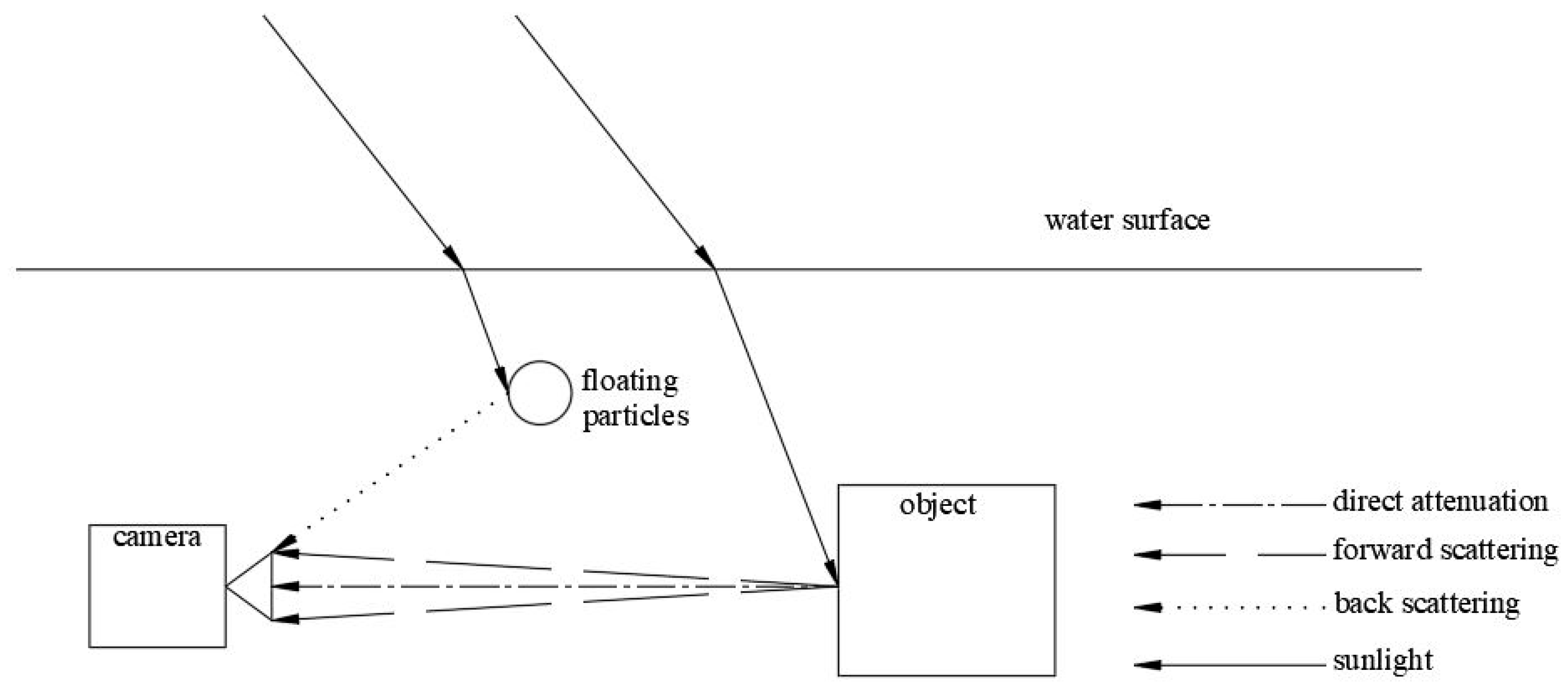
3. Background

Underwater images are generally degraded due to the absorption and scattering of light. The medium of water causes the absorption of light, reducing the energy of light based on its wavelength and depth. As different wavelengths of light have varying attenuation rates in water, this leads to color distortion. In addition, the scattering of light is caused by suspended particles in the water reflecting light in other directions, resulting in image blurring. The Jaffe–McGlamery underwater imaging model suggests that the light received by the camera in an underwater scene contains three components: the direct attenuation component, the forward scattering component, and the backscattering component, as shown in Figure 2. Therefore, an underwater image can be represented as a linear superposition of these three components. The model can be expressed as

$$E_T=E_d+E_f+E_b$$

(1)

where $E_T$ is the light arriving at the camera, $E_d$ is the direct attenuation, $E_f$ is the forward scattering, and $E_b$ is the backscattering.

Figure 2. Jaffe–McGlamery underwater imaging model.

Direct attenuation is the attenuation due to the main radiation within the medium with increasing propagation distance. It is mathematically defined as

$$E_d\left(x,\lambda \right)=J\left(x,\lambda \right)t\left(x,\lambda \right),\lambda \in \{\mathrm{R},\mathrm{G},\mathrm{B}\}$$

(2)

where x denotes a pixel, $\lambda$ is the wavelength of light, $J\left(x,\lambda \right)$ is the non-degraded image, and $t\left(x,\lambda \right)$ is the transmission map.

Forward scattering is the light reflected from the target object that reaches the camera through scattering. It can be expressed as

$$E_f\left(x,\lambda \right)=E_d\left(x,\lambda \right) \ast g_d\left(x\right),\lambda \in \{\mathrm{R},\mathrm{G},\mathrm{B}\}$$

(3)

where $g_d\left(x\right)$ is the point spread function; because forward scattering has little effect on image quality, it is usually neglected.

Backscattering is the light reaching the camera due to the scattering effect of impurities in the water. It can be expressed as

$$E_b\left(x,\lambda \right)=B_{\infty }\left(\lambda \right)(1-t\left(x,\lambda \right)),\lambda \in \{\mathrm{R},\mathrm{G},\mathrm{B}\}$$

(4)

where $B_{\infty }\left(\lambda \right)$ is the background light, it represents the color of the body of water, and its value can be expressed as the grayscale value of a point at a distance of infinity from the camera.

The simplified underwater imaging model [25] can be expressed as

$$I\left(x,\lambda \right)=J\left(x,\lambda \right)t\left(x,\lambda \right)+B_{\infty }\left(\lambda \right)(1-t\left(x,\lambda \right)),\lambda \in \{\mathrm{R},\mathrm{G},\mathrm{B}\}$$

(5)

where $I\left(x,\lambda \right)$ is the observed image.

Equation (5) can be transformed into Equation (6). The main task of underwater image recovery is to estimate the transmission map $t\left(x,\lambda \right)$ and the background light $B_{\infty }\left(\lambda \right)$.

$$J\left(x,\lambda \right)=\frac{I\left(x,\lambda \right)-B_{\infty }\left(\lambda \right)(1-t\left(x,\lambda \right))}{t\left(x,\lambda \right)},\lambda \in \{\mathrm{R},\mathrm{G},\mathrm{B}\}$$

(6)

Methods for solving the background light and the transmission map often involve estimating the distance between the camera and the target. This is because the background light represents the grayscale value of a point at infinity from the camera. In addition, according to the Beer–Lambert law [29], as shown in Equation (7), the transmission map decreases exponentially as the distance increases.

$$t\left(x,\lambda \right)={\mathrm{e}}^{-\mathrm{c}d\left(x\right)},\lambda \in \{\mathrm{R},\mathrm{G},\mathrm{B}\}$$

(7)

where c is the attenuation coefficient; d(x) is the distance between the camera and the target.

4. The Proposed Method

In this section, this paper will introduce the proposed method for restoring overhead underwater images, as well as strategies for accelerating the process. The operational steps of the proposed method are shown in Figure 3. Firstly, the transmission map is calculated, and the values of the transmission map outside the range are transferred by a translation function to reduce information loss. Secondly, the background light for the blue and green channels is estimated by minimizing the loss function. Thirdly, the background light for the red channel is determined based on the principle of minimizing the average grayscale difference between the three channels. Finally, the degraded underwater image can be restored based on the obtained background light and transmission map.

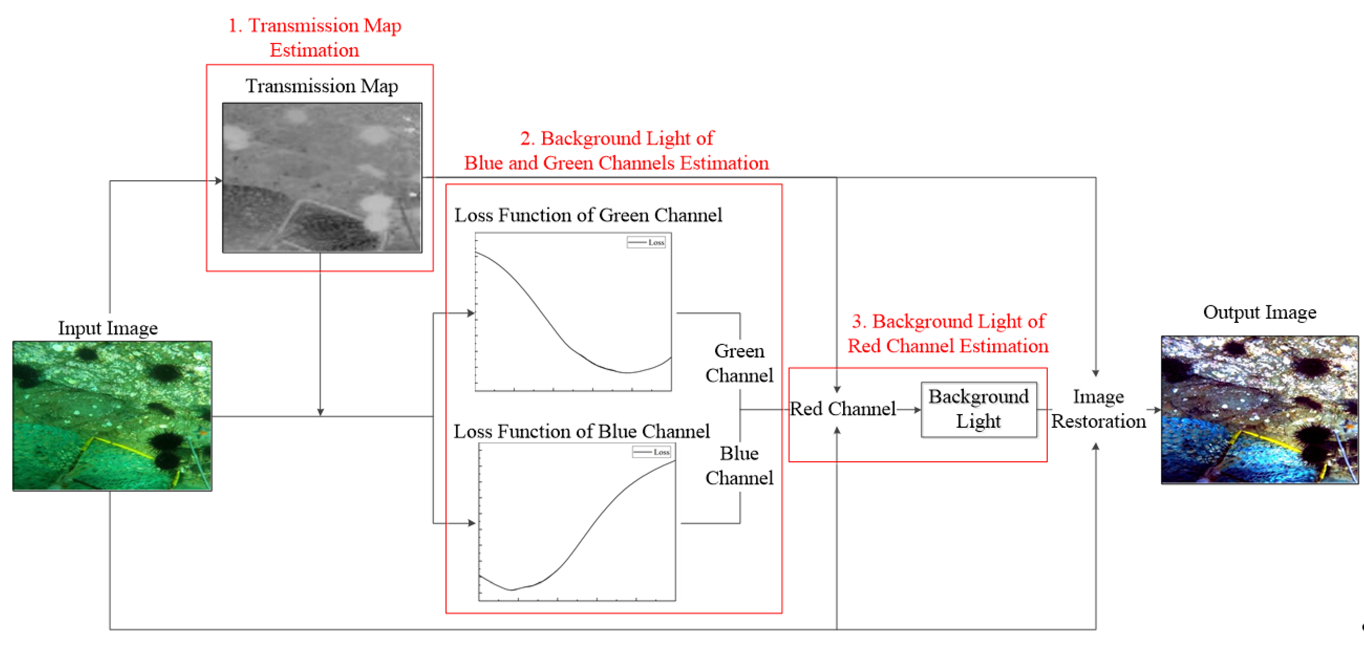
Figure 3. Operation process of the proposed method.

4.1. Transmission Map Estimation

To achieve accurate transmission map solutions and avoid compounding errors, this paper utilizes the MIP algorithm’s [1] transmission map solution method instead of the DCP algorithm, which depends on the background light. In the MIP algorithm, the largest differences among the three different color channels are calculated as follows:

$$D\left(x\right)=\underset{x\in \mathit{\Omega }, \lambda =\mathrm{R}}{\max }I\left(x,\lambda \right)-\underset{x\in \mathit{\Omega }, \lambda \in \{\mathrm{B},\mathrm{G}\}}{\max }I\left(x,\lambda \right)$$

(8)

where $D\left(x\right)$ is the largest difference among the three color channels, and $\mathit{\Omega }$ is a local patch in the image.

The transmission map is

$$t\left(x\right)=D\left(x\right)+(1-\underset{x}{\max }D\left(x\right))$$

(9)

As shown by Equation (5), t(x) and (1 − t(x)), respectively, represent the contribution of the main radiation and the background radiation to the image. The value of t(x) decreases as the background radiation dominates the grayscale value. However, as the background radiation is usually not as bright as the main radiation, the minimum value of t(x) is kept at 0.1 to avoid an overly dark recovered image. In addition, to preserve the image’s authenticity, a portion of the fog is retained in the recovered image. Hence, the maximum value of t(x) is set to 0.95 [5]. This leads to a transmission map range of [0.1, 0.95].

However, simply cutting off the transmission map values beyond the range of values will lead to the loss of information. Therefore, in this paper, the transmission map is transformed as follows to transfer the information in the transmission map to the range [0.1, 0.95] as much as possible.

$$\begin{gathered} \tau =\left\{\begin{array}{cc}\hfill \min (t_{max}-0.95,t_{min}-0.1),& \mid \hspace{1em}{t}_{max}>0.95,t_{min}>0.1\hfill \\ \hfill -\min (0.95-t_{max},0.1-t_{min}),& \mid \hspace{1em}{t}_{max}<0.95,t_{min}<0.1\hfill \\ \hfill 0,& \hspace{1em}\mathrm{otherwise}\hfill \end{array}\right. \\ {t}_{trans}\left(x\right)=t\left(x\right)-\tau \end{gathered}$$

(10)

where $\tau$ is the quantity of the transformation, $t_{min}$ is the minimum value of the transmission map, $t_{max}$ is the maximum value of the transmission map, and $t_{trans}\left(x\right)$ is the transmission map after the transformation.

This transformation technique retains some transmission map information beyond the effective range while maintaining the contrast of the original transmission map. The comparison results of the transmission maps before and after the transformation are depicted in Figure 4a,b. The entropy values of the transmission maps are 5.5424 and 5.5433, respectively, indicating that the transformed transmission map is more detailed and informative.

Figure 4. (a) Transmission map before transfer; (b) Transmission map after transfer.

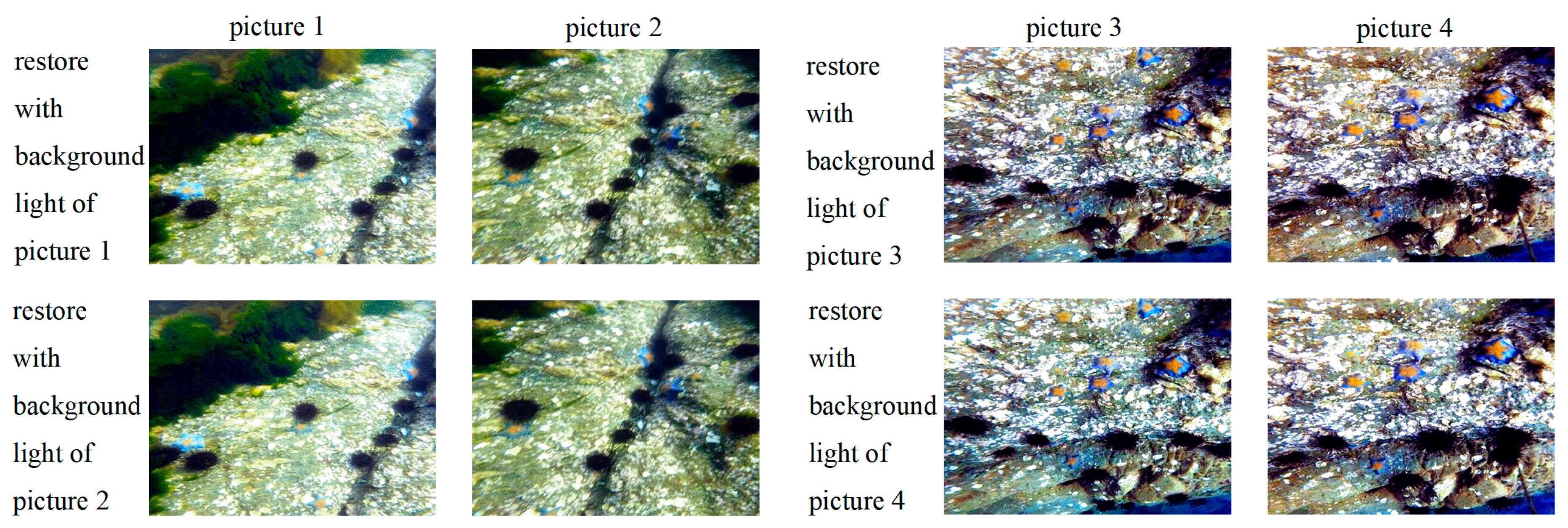
4.2. Background Light of Blue and Green Channels Estimation

As mentioned above, it is not appropriate to use one or the mean value of a few pixels in the image to represent the background light in an overhead image because there is no point far enough in the image that can be reasonably approximated as background light. To overcome this limitation, this paper calculates the value of the background light through inference rather than relying on any specific pixel value in the image. The value of the background light is inferred from the desired image result, which provides a more accurate representation of the background light.

Firstly, motivated by Li et al. [30], who determined the transmission map by minimizing information loss, this paper aims to find the background light by minimizing the information loss of the image. To ensure that the grayscale value of the restored image is between 0 and 1, any values outside this range are directly assigned to 0 or 1. If there are too many pixels outside the grayscale range, large black or white areas will appear in the image, leading to information loss from the original image.

To solve this problem, the existing approach is to use the stretching function.

$$S\left(v\right)=\frac{v-\min \left(V\right)}{\max \left(V\right)-\min \left(V\right)}$$

(11)

where V represents the grayscale range before stretching and v represents the grayscale value involved in the calculation.

The grayscale difference between the two pixels can be expressed as

$$\begin{gathered} \Delta v=v_1-v_2 \\ \Delta v_s=\frac{\Delta v}{\max \left(V\right)-\min \left(V\right)} \end{gathered}$$

(12)

where $\mathsf{\Delta }v$ represents the difference between the two pixels before stretching, and $\mathsf{\Delta }{v}_s$ represents the difference between the two pixels after stretching.

While the method is effective when the difference between the maximum and minimum grayscale values is less than 1, it is unsuitable for cases where this difference exceeds 1. In such scenarios, the method compresses the original grayscale values, resulting in decreased contrast between pixels. This can lead to loss of important information and reduced overall image quality. Therefore, compressing the contrast of the entire image to retain a few bright or dark pixels that contain minimal information is not a reasonable approach.

When the grayscale difference $\max \left(V\right)-\min \left(V\right)$ is greater than 1, the method described above directly assigns the under or over the part to 0 or 1. However, to minimize information loss and maintain the contrast of the image, this paper aims to minimize the number of pixels that fall outside the grayscale range. In other words, the number of such pixels must be kept as small as possible while minimizing the information loss.

$$\min (\mathrm{M} \mathrm{\ast } \mathrm{N}-n_{J{b}_i\left[\mathrm{0,1}\right]}\left(\lambda \right)),\lambda \in \{\mathrm{G},\mathrm{B}\}$$

(13)

where M and N represent the length and width of the image and $n_{J{b}_i\left[\mathrm{0,1}\right]}\left(\lambda \right)$ is the number of pixels whose grayscale values fall between 0 and 1 in the image recovered by taking the background light $b_i$.

In addition, Li et al. [30] observed that the histograms of clear, fog-free images are distributed relatively uniformly without sharp points, based on their analysis of image datasets of five natural scenes. However, the histograms of underwater images are typically concentrated in a small range. In light of this, the present study aims to produce restored images with the most balanced grayscale distribution. This is achieved by minimizing the variance of the histogram of the restored image, which can be expressed as

$$\min \left(S_{over}\left(\lambda \right)\right),\lambda \in \{\mathrm{G},\mathrm{B}\}$$

(14)

where $S_{over}\left(\lambda \right)$ is the area of the histogram of the recovered images over the desired histogram (the desired histogram is the most uniform distribution of image grayscale, with the same number of pixels falling on each gray value as (M × N)/255), indicating the degree of unevenness of the histogram distribution, as shown in Figure 5.

Figure 5. The area of $S_{over}\left(\lambda \right)$.

In summary, the loss function for obtaining the background light values in the range [0, 1] is defined as follows:

$$Loss\left(b_i,\lambda \right)==\mathrm{M} \mathrm{\ast } \mathrm{N}-n_{J{b}_i\left[\mathrm{0,1}\right]}\left(\lambda \right)+S_{over}\left(\lambda \right),\lambda \in \left\{\mathrm{G},\mathrm{B}\right\}$$

(15)

Then the background light of the blue and green channels is

$${\mathrm{B}}_{\mathrm{\infty }}\left(\mathsf{\lambda }\right)=\underset{b_i}{\mathrm{argmin}}Loss\left(b_i,\lambda \right),\lambda \in \{\mathrm{G},\mathrm{B}\}$$

(16)

Through several experiments, it is found that the loss function is generally convex, i.e., it shows a trend of decreasing and then increasing as the background light $b_i$ increases, as shown in Figure 6. Therefore, inspired by the loss function optimization method in deep learning, to find the background light that makes the loss function obtain the minimum value, instead of finding all the function values within the range of values of background light $b_i$, the gradient descent method can be used, as shown in Equation (17), and $B_{\infty }\left(\lambda \right)$ can be obtained after several steps.

$$b_{i+1}\left(\lambda \right)=b_i-ϵ\frac{\partial Loss\left(b_i,\lambda \right)}{\partial b_i}$$

(17)

where $ϵ$ is the learning rate.

Figure 6. The shape of the loss function.

4.3. Background Light of Red Channel Estimation

Due to the red channel’s limited information, it is challenging to accurately determine the background light using only this channel. Therefore, this paper infers the red channel background light by leveraging information from the recovered blue-green channels. The study analyzes the mean values of the red, green, and blue channels of both natural and underwater image datasets, as illustrated in Figure 7 and Figure 8. The details of the datasets are as follows:

Figure 7. The mean values of the red, green, and blue channels of the natural image dataset.

Figure 8. The mean values of the red, green, and blue channels of the underwater image dataset.

• The Caltech-UCSD Birds-200-2011 Dataset (http://www.vision.caltech.edu/datasets/cub_200_2011/, accessed on 20 March 2023) [31]. This is a natural image dataset for bird image classification, which includes 11,788 images covering 200 bird species.
• CBCL Street Scenes Dataset (http://cbcl.mit.edu/software-datasets/streetscenes/, accessed on 20 March 2023) [32]. This is a dataset of street scene images captured by a DSC-F717 camera from Boston and its surrounding areas in Massachusetts, belonging to the category of natural image datasets, with a total of 3547 images.
• Real World Underwater Image Enhancement dataset (https://github.com/dlut-dimt/Realworld-Underwater-Image-Enhancement-RUIE-Benchmark, accessed on 20 March 2023) [33]. This underwater image dataset was collected from a real ocean environment testing platform consisting of 4231 images. The dataset is characterized by its large data size, diverse degree of light scattering effects, rich color tones, and abundant detection targets.

The natural images exhibit similar three-channel mean values, whereas the underwater images demonstrate a clear demarcation. To further investigate this difference, Equation (18) calculates the sum of the differences between the three-channel means, and Figure 9 displays the results. The analysis shows that the $D_{RGB}$ values for underwater images are significantly larger than those for natural images.

$$D_{RGB}=|\overline{I_R}-\overline{I_B}|+|\overline{I_R}-\overline{I_G}|+|\overline{I_G}-\overline{I_B}|$$

(18)

where $\overline{I_R}$, $\overline{I_B}$, and $\overline{I_G}$ are the mean values of the red, green, and blue channels of the observed image.

Figure 9. The $D_{RGB}$ values of the underwater and natural images.

Therefore, this paper aims to minimize the $D_{RGB}$ values. Specifically, the gray mean value of the blue and green channels is utilized as the gray mean value of the red channel to derive the red channel background light. This approach allows for correcting the color shift problem in underwater images without additional image enhancement operations.

$$\begin{gathered} \overline{J_{\mathrm{R}}}=\frac{\overline{J_{\mathrm{B}}}+\overline{J_{\mathrm{G}}}}{2} \\ {B}_{\infty }\left(R\right)=\frac{\overline{I_R}-\overline{J_R}\times \overline{t}}{1-\overline{t}} \end{gathered}$$

(19)

where $\overline{J_{\mathrm{R}}}$, $\overline{J_{\mathrm{B}}}$, and $\overline{J_{\mathrm{G}}}$ are the mean values of the red, green, and blue channels of the restored image, $\overline{t}$ is the mean value of the transmission map.

In some cases, there may be a significant difference between the mean value of the blue channel $\overline{J_{\mathrm{B}}}$ and the mean value of the green channel $\overline{J_{\mathrm{G}}}$, leading to a color bias towards red in the resulting image. To address this issue, this paper proposes a solution where the background light of the channel with the higher mean value is kept, and its recovery map is used to estimate the background light of the remaining two channels. For instance, if the mean value of the green channel is larger, the background light of the other two channels can be estimated as follows:

$$\begin{gathered} B_{\infty }\left(R\right)=\frac{\overline{I_R}-\overline{J_G}\times \overline{t}}{1-\overline{t}} \\ {B}_{\infty }\left(B\right)=\frac{\overline{I_B}-\overline{J_G}\times \overline{t}}{1-\overline{t}} \end{gathered}$$

(20)

The recovered image is obtained by bringing the transmission map and background light into Equation (6).

4.4. Strategies to Speed Up

Considering the need for higher computational efficiency, this paper aims to improve the operation speed by addressing two key factors: the spatial resolution of images and the similarity of neighboring images.

First, the proposed background light calculation method is based on the global consideration of the picture and is not sensitive to the size of the picture. As shown in Figure 10, the recovery effect of the picture is not affected too much after reducing the size of the picture to 1/K of the original one. Therefore, when applied in practice, the K value can be adjusted appropriately, weighing the imaging effect as well as the running speed.

Figure 10. Results of image restoration using the background light were calculated by reducing the image by a factor of K.

Second, in the continuous working state, the scene of several adjacent frames does not change much, and the background light values can be shared to further improve the running speed. As shown in Figure 11, the recovery images are almost the same after the neighboring images swap the background light values.

Figure 11. The results of image restoration by sharing the background light between several adjacent frames.

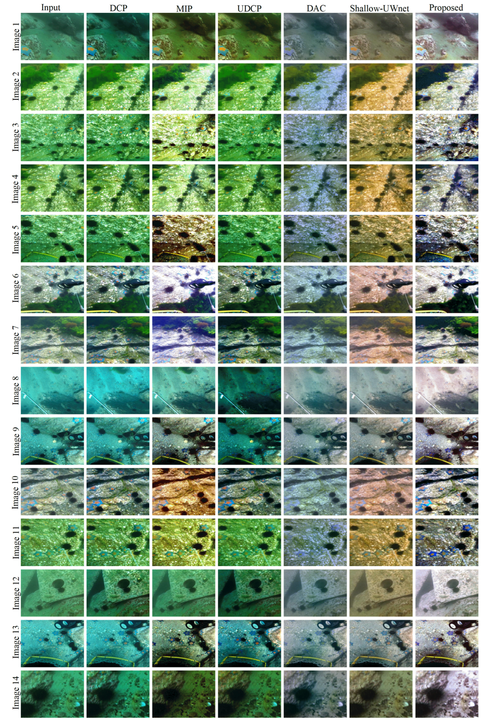
5. Experimental Results and Discussion

The proposed approach is compared with five existing techniques: the dark channel prior (DCP) method [5], underwater dark channel prior (UDCP) method [6], Carlevaris-Bianco’s (MIP) method [1], Differential Attenuation Compensation (DAC) method [2] and Shallow-UWnet method [34]. Underwater images were obtained from the Real World Underwater Image Enhancement dataset [33]. Qualitative and quantitative evaluations are carried out to assess the performance of different methods.

In this study, different types of images are selected from the dataset (including images with the green tune, blue tune, and images with less color bias). In addition, the performance of the proposed method is compared with other methods in restoring real underwater images. Qualitative experiments show the results of different methods in restoring underwater aerial images, as shown in Figure 12. The proposed method eliminates the effects of light absorption, corrects the color distortion of blue-green color cast in underwater images, and restores the rich and vibrant colors of the images, which is in line with common sense. In addition, the proposed method successfully eliminates the effects of scattering and makes the images clearer. Other methods improve the underwater images to different extents but still have room for improvement. Although the DCP and UDCP methods improve the clarity of the images, they do not correct the color bias of the images. The MIP method successfully performs defogging of the images but causes undesirable yellow color bias. DAC algorithm overcomes the color bias problem. However, the restored images are more blurry than other methods, and the corrected colors are relatively dim. The Shallow-UWnet algorithm successfully corrects the color bias of blue tune underwater images. Still, for images with green tune or less color bias, the restored images are over-corrected, resulting in additional yellow or red color distortion. Therefore, their method’s results are not satisfactory. The fact that every point in the underwater aerial image is near the camera is considered. The proposed method does not use distance-based background light solutions but instead chooses the best global solution for background light. As a result, the method produces more natural and superior results in terms of color and detail than other methods.

Figure 12. Subjective evaluation results.

Table 1 shows the average processing time and hardware requirements for different algorithms to process one image, as well as their integrated development environments (IDE). The DCP method [5], UDCP method [6], MIP method [1], DAC method [2], and the proposed method run on the Windows 10 operating system, with 16 GB of memory and 11th Gen Intel(R) Core(TM) i7-1165G7 @ 2.80 GHz (8 CPUs). The Shallow-UWnet method [34] runs on a Tesla T4 GPU. As shown in Table 1, among the algorithms running on the CPUs, the DCP algorithm has the fastest speed. The proposed method in this paper is slightly slower than MIP and UDCP. The Shallow-UWnet algorithm has good real-time performance but requires additional hardware resources.

Table 1. The average processing time, hardware requirements, and IDE of each method.

Algorithm	DCP	MIP	UDCP	DAC	Shallow-UWnet	Proposed
Time (s)	0.1822	0.2493	0.2166	1.7272	0.2227	0.3345
IDE	Pycharm	Pycharm	Pycharm	MATLAB	Pycharm	Pycharm
Hardware	CPU	CPU	CPU	CPU	GPU	CPU

To show the proposed method’s advantages quantitatively, comparisons are made with other restoration methods using three underwater quality evaluation metrics: the Underwater Color Image Quality Evaluation Metric (UCIQE) [35], the Underwater Image Quality Measure (UIQM) [36], and the entropy.

UCIQE is an objective evaluation expressed as a linear combination of chroma, saturation, and contrast:

$$UCIQE=m_1\times {\sigma }_c+m_2\times co{n}_l+m_3\times {\mu }_s$$

(21)

where $m_1$,$m_2$, and $m_3$ are the scale factors, they are set as per the original paper [35]. ${\sigma }_c$ is the standard deviation of chroma, $co{n}_l$ is the contrast of brightness, and ${\mu }_s$ is the saturation average.

UIQM evaluates the quality of underwater images through a linear combination of its three components: sharpness measure, colorfulness measure, and contrast measure.

$$UIQM=c_1\times UICM+c_2\times UISM+c_3\times UIConM$$

(22)

where $c_1$, $c_2$, and $c_3$ are the scale factors, they are set as per the original paper [36]. UICM is the colorfulness measure, UISM is the sharpness measure, and UIConM is the contrast measure.

The entropy of the system reflects the degree of chaos, and the higher the entropy, the more information the image contains, which means the clearer the image.

Table 2 and Table 3 report the UCIQE and UIQM scores of images shown in Figure 12. The scores in bold denote the best results. The proposed method has stronger robustness and optimal overall performance in various scenarios, as indicated by its maximum average value. While the UCIQE and UIQM scores for some of the images processed by the proposed method were slightly lower than those of other methods, these methods exhibited larger fluctuations, with high scores in some images and low scores in others. In contrast, the proposed method demonstrates a more stable restoration performance for various types of images. However, it should be noted that some of the restoration images with higher scores were too focused on enhancing contrast, neglecting color correction.

Table 2. UCIQE scores * of images shown in Figure 12.

Image	Origin	DCP	MIP	UDCP	DAC	Shallow-UWnet	Proposed
1	0.2722	0.3790	0.3730	0.3947	0.2255	0.2290	0.3896
2	0.3609	0.3917	0.3808	0.4015	0.3874	0.3967	0.4234
3	0.3751	0.407	0.4285	0.4222	0.3491	0.3779	0.4568
4	0.3752	0.4053	0.3771	0.4175	0.3679	0.4026	0.4099
5	0.4298	0.4385	0.4961	0.4587	0.4022	0.4185	0.4968
6	0.3630	0.4035	0.4137	0.4510	0.3589	0.4545	0.4916
7	0.3224	0.408	0.3533	0.4583	0.3122	0.4183	0.4616
8	0.375	0.4149	0.3632	0.4910	0.2577	0.2555	0.3985
9	0.4489	0.4572	0.4625	0.5156	0.3707	0.3927	0.5052
10	0.3888	0.4174	0.4588	0.434	0.3617	0.3967	0.4479
11	0.3148	0.4020	0.4987	0.4295	0.2966	0.4397	0.4671
12	0.2854	0.3990	0.3106	0.3835	0.2149	0.2366	0.3536
13	0.4681	0.4708	0.4680	0.5152	0.3664	0.3709	0.4964
14	0.3713	0.4125	0.3947	0.3605	0.3109	0.2725	0.4265
Average	0.3679	0.4148	0.4128	0.4381	0.3273	0.3616	0.4446

* A higher UCIQE score indicates better image quality.

Table 3. UIQM scores * of images shown in Figure 12.

Image	Origin	DCP	MIP	UDCP	DAC	Shallow-UWnet	Proposed
1	−0.8400	−0.2123	−0.2165	−0.3135	−0.8632	−0.3081	−0.2368
2	−0.2399	0.1390	−0.2809	0.2300	−0.3355	−0.0169	0.1813
3	0.0389	0.4613	0.5522	0.6048	−0.2648	0.0105	0.9704
4	−0.2021	0.1858	−0.2702	0.2522	−0.3302	−0.0475	0.2504
5	0.2519	0.4889	1.5800	0.6816	−0.1267	0.2372	1.4260
6	−0.3721	0.0374	0.2101	0.3436	−0.4271	−0.2427	0.5991
7	−0.5682	−0.1038	−0.0442	0.4378	−0.5846	−0.4666	0.3336
8	−0.2644	0.1885	−0.3574	0.6283	−0.6318	−0.649	−0.2960
9	0.3213	0.3925	0.9095	0.892	−0.1506	−0.1994	0.7112
10	−0.0872	0.3457	0.6865	0.4386	−0.3144	−0.0487	0.7507
11	−0.4421	0.1594	0.9140	0.5198	−0.4638	−0.4826	0.8586
12	−0.6686	−0.2113	−0.6194	0.0549	−0.7350	−0.4215	−0.2384
13	0.4338	0.5377	1.1882	1.0858	−0.2229	−0.3031	0.6632
14	−0.4251	−0.0212	0.3275	−0.3393	−0.4701	−0.3526	−0.3487
Average	−0.2188	0.1705	0.3271	0.394	−0.4229	−0.2351	0.4018

* A higher UIQM score suggests that the result is more consistent with human visual perception.

To further demonstrate the superiority of the proposed method in color correction, the colorfulness measures in UCIQE and UIQM scores (${\sigma }_c$ and UICM) are additionally listed in Table 4 and Table 5. The results show that the proposed method achieved the highest or near-highest scores in both evaluation metrics, indicating that the algorithm can effectively improve the color level of the restored images. This is because the histogram distribution balance was considered when constructing the loss function, and the value of the background light was obtained by minimizing the loss function. Therefore, the calculated background light can make the restored images more colorful and vivid.

Table 4. The colorfulness measure ${\sigma }_c$ * in UCIQE scores of images shown in Figure 12.

Image	Origin	DCP	MIP	UDCP	DAC	Shallow-UWnet	Proposed
1	0.0291	0.0393	0.0446	0.0447	0.0646	0.0569	0.2923
2	0.0387	0.0454	0.0688	0.0372	0.1490	0.0346	0.2191
3	0.0329	0.0387	0.0824	0.033	0.1026	0.0264	0.261
4	0.0349	0.0434	0.054	0.0368	0.1175	0.0215	0.2474
5	0.0344	0.0370	0.1401	0.034	0.1171	0.0376	0.2812
6	0.0869	0.1049	0.2182	0.1091	0.1028	0.2900	0.2728
7	0.1088	0.1149	0.1598	0.1152	0.0934	0.2792	0.2269
8	0.0113	0.0120	0.0229	0.0368	0.049	0.0772	0.3443
9	0.0458	0.0434	0.2114	0.0746	0.0987	0.1818	0.3464
10	0.0428	0.0515	0.0601	0.0419	0.1015	0.0332	0.2266
11	0.114	0.1353	0.1437	0.1331	0.0669	0.3108	0.2602
12	0.0211	0.0467	0.0259	0.0484	0.0573	0.0176	0.2991
13	0.0643	0.0582	0.1629	0.1207	0.1053	0.1563	0.331
14	0.0174	0.0275	0.0826	0.0517	0.0915	0.0346	0.294
Average	0.0487	0.0570	0.1055	0.0655	0.0941	0.1113	0.2787

* A higher ${\sigma }_c$ score indicates richer colors in the image.

Table 5. The colorfulness measure UICM * in UIQM scores of images shown in Figure 12.

Image	Origin	DCP	MIP	UDCP	DAC	Shallow-UWnet	Proposed
1	−0.7381	−0.3839	3.7792	2.2919	−1.9772	17.6672	17.2558
2	4.9669	5.4557	4.0874	5.0828	9.0464	14.4282	14.5248
3	5.3565	5.3235	8.2615	4.7840	5.2131	14.7446	16.8768
4	3.7914	4.5229	2.7446	4.2913	6.3745	9.9716	17.1822
5	4.8659	4.5921	15.3959	4.1764	4.9793	17.2987	17.6408
6	4.9898	5.6814	15.6180	4.9501	5.3688	14.4294	17.4807
7	4.8346	4.3226	15.9747	3.6215	4.5631	9.7244	15.6106
8	4.9449	5.0272	5.2024	0.7624	3.5792	4.2325	15.1843
9	5.4198	4.8146	13.1484	3.4475	5.7817	13.3738	17.2481
10	5.0785	5.2059	8.3004	4.8098	5.1170	11.5138	17.2416
11	5.0306	6.2061	8.2831	5.7368	4.1944	7.3071	17.4254
12	3.5741	1.4052	1.7001	−1.3721	1.6424	14.6708	16.9075
13	6.2110	5.7990	11.1680	6.4725	5.4693	9.8003	18.1152
14	0.9821	1.8303	7.3491	0.2730	2.7675	13.1950	10.2711
Average	4.2363	4.2716	8.6438	3.5234	4.4371	12.3112	16.3546

* A higher UICM score indicates a more balanced color in the image.

Table 6 gives the entropy values of the images shown in Figure 12. The images restored by the proposed method carry more information. This is because the transformation function in this study preserved more information about the transmitted image, and the loss of information was considered when constructing the loss function. This allows the calculated background light to retain more information about the image.

Table 6. Entropy * values of images shown in Figure 12.

Image	Origin	DCP	MIP	UDCP	DAC	Shallow-UWnet	Proposed
1	6.4746	6.6325	6.993	6.9564	6.4891	6.4818	7.4472
2	7.5963	7.5738	7.7616	7.5553	7.3026	7.4749	7.8655
3	7.3334	7.459	7.7236	7.3815	7.1283	7.2481	7.7627
4	7.5308	7.6079	7.7275	7.5382	7.2805	7.4499	7.8300
5	7.5362	7.4825	7.8325	7.4762	7.3261	7.4873	7.7172
6	7.5771	7.6552	7.4784	7.5963	7.502	7.4921	7.6124
7	7.4291	7.3635	7.7968	7.5028	7.2571	7.3375	7.9253
8	6.765	6.9913	7.1735	6.4368	6.8517	6.7923	7.4940
9	7.5079	7.4011	7.7481	7.219	7.5068	7.4889	7.8966
10	7.2536	7.4224	7.6655	7.3088	7.0689	7.1571	7.6892
11	7.3948	7.6695	7.8462	7.6124	7.2622	7.2871	7.7604
12	6.659	7.1119	6.7411	6.7670	6.6057	6.6583	7.3675
13	7.4904	7.431	7.5626	7.6088	7.4993	7.4456	7.9022
14	6.9208	6.9743	6.7258	6.7058	7.0053	6.9624	7.8121
Average	7.2478	7.3411	7.484	7.2618	7.149	7.1974	7.7202

* A higher entropy value suggests that the result contains more information.

6. Conclusions

In this paper, a new image recovery method has been proposed for overhead images taken by UUVs performing tasks such as underwater pipeline tracking, underwater mine clearance, underwater terrain detection, and seafood fishing. Firstly, a distance-independent background light calculation method has been proposed for the overhead images where the points are close to the camera, unlike the previous methods that use the most distant point in the image to approximate the background light. Next, an optimization function based on the overall information loss as well as the uniformity of the histogram distribution has been used to calculate the blue and green channel background light values. Then, based on the statistical results, the mean value of the red channel has been determined based on the principle of minimizing the sum of the differences between the mean values of the three channels, which has been used to invert the background light value of the red channel. Moreover, this paper also has used the translation function to control the value range of the transmission map between 0.1 and 0.95, which retains the information carried by the transmission map. Finally, based on the real-time consideration, two strategies have been proposed to speed up the operation from the perspective of the spatial resolution of the image and the similarity of two adjacent frames. The experimental results show that the proposed method has strong robustness in adapting to various underwater environments. Moreover, the method can effectively correct the blue-green color cast in underwater images while preserving more information. Importantly, the method can run on a CPU without the need for additional hardware resources. The average processing time per frame is 0.3345 s, demonstrating good real-time performance.

However, the proposed method still has some limitations. The method focuses on color restoration and information preservation without taking measures to enhance contrast. In future work, efforts will be made to enhance the contrast of underwater images to make image details clearer.

References

- Carlevaris-Bianco, N.; Mohan, A.; Eustice, R.M. Initial results in underwater single image dehazing. In Proceedings of the Oceans 2010 Mts/IEEE Seattle, Seattle, WA, USA, 20–23 September 2010; pp. 1–8. [Google Scholar]
- Lai, Y.; Zhou, Z.; Su, B.; Zhe, X.; Tang, J.; Yan, J.; Liang, W.; Chen, J. Single underwater image enhancement based on differential attenuation compensation. Front. Mar. Sci. 2022, 9, 1047053. [Google Scholar] [CrossRef]
- McGlamery, B. A computer model for underwater camera systems. In Proceedings of the Ocean Optics VI; SPIE: Bellingham, WA, USA, 1980; pp. 221–231. [Google Scholar]
- Jaffe, J.S. Computer modeling and the design of optimal underwater imaging systems. IEEE J. Ocean. Eng. 1990, 15, 101–111. [Google Scholar] [CrossRef]
- He, K.; Sun, J.; Tang, X. Single Image Haze Removal Using Dark Channel Prior. IEEE Trans. Pattern Anal. Mach. Intell. 2011, 33, 2341–2353. [Google Scholar] [CrossRef] [PubMed]
- Drews, P., Jr.; do Nascimento, E.; Moraes, F.; Botelho, S.; Campos, M. Transmission Estimation in Underwater Single Images. In Proceedings of the 2013 IEEE International Conference on Computer Vision Workshops, Sydney, Australia, 2–8 December 2013; pp. 825–830. [Google Scholar]
- Song, W.; Wang, Y.; Huang, D.; Tjondronegoro, D. A rapid scene depth estimation model based on underwater light attenuation prior for underwater image restoration. In Proceedings of the Pacific Rim Conference on Multimedia, Hefei, China, 21–22 September 2018; pp. 678–688. [Google Scholar]
- Li, C.; Quo, J.; Pang, Y.; Chen, S.; Wang, J. Single underwater image restoration by blue-green channels dehazing and red channel correction. In Proceedings of the 2016 IEEE International Conference on Acoustics, Speech and Signal Processing (ICASSP), Shanghai, China, 20–25 March 2016; pp. 1731–1735. [Google Scholar]
- Liang, Z.; Wang, Y.; Ding, X.; Mi, Z.; Fu, X. Single underwater image enhancement by attenuation map guided color correction and detail preserved dehazing. Neurocomputing 2021, 425, 160–172. [Google Scholar] [CrossRef]
- Ding, X.; Liang, Z.; Wang, Y.; Fu, X. Depth-aware total variation regularization for underwater image dehazing. Signal Process. Image Commun. 2021, 98, 116408. [Google Scholar] [CrossRef]
- Emberton, S.; Chittka, L.; Cavallaro, A. Underwater image and video dehazing with pure haze region segmentation. Comput. Vis. Image Underst. 2018, 168, 145–156. [Google Scholar] [CrossRef]
- Ancuti, C.O.; Ancuti, C.; De Vleeschouwer, C.; Sbetr, M. Color Channel Transfer for Image Dehazing. IEEE Signal Process. Lett. 2019, 26, 1413–1417. [Google Scholar] [CrossRef]
- Li, T.; Wang, J.; Yao, K. Visibility enhancement of underwater images based on active polarized illumination and average filtering technology. Alex. Eng. J. 2022, 61, 701–708. [Google Scholar] [CrossRef]
- Dai, C.; Lin, M.; Wu, X.; Wang, Z.; Guan, Z. Single underwater image restoration by decomposing curves of attenuating color. Opt. Laser Technol. 2020, 123, 105947. [Google Scholar] [CrossRef]
- Peng, Y.-T.; Cosman, P.C. Underwater image restoration based on image blurriness and light absorption. IEEE Trans. Image Process. 2017, 26, 1579–1594. [Google Scholar] [CrossRef]
- Ke, K.; Zhang, C.; Wang, Y.; Zhang, Y.; Yao, B. Single underwater image restoration based on color correction and optimized transmission map estimation. Meas. Sci. Technol. 2023, 34, 055408. [Google Scholar] [CrossRef]
- Wang, X.; Tao, C.; Zheng, Z.J.O.; Engineering, L.i. Occlusion-aware light field depth estimation with view attention. Opt. Lasers Eng. 2023, 160, 107299. [Google Scholar] [CrossRef]
- Zhan, F.; Yu, Y.; Zhang, C.; Wu, R.; Hu, W.; Lu, S.; Ma, F.; Xie, X.; Shao, L. Gmlight: Lighting estimation via geometric distribution approximation. IEEE Trans. Image Process. 2022, 31, 2268–2278. [Google Scholar] [CrossRef]
- Wang, Y.; Yu, X.; An, D.; Wei, Y. Underwater image enhancement and marine snow removal for fishery based on integrated dual-channel neural network. Comput. Electron. Agric. 2021, 186, 106182. [Google Scholar] [CrossRef]
- Wang, K.; Shen, L.; Lin, Y.; Li, M.; Zhao, Q. Joint Iterative Color Correction and Dehazing for Underwater Image Enhancement. IEEE Robot. Autom. Lett. 2021, 6, 5121–5128. [Google Scholar] [CrossRef]
- Zong, X.; Chen, Z.; Wang, D.J.A.I. Local-CycleGAN: A general end-to-end network for visual enhancement in complex deep-water environment. Appl. Intell. 2021, 51, 1947–1958. [Google Scholar] [CrossRef]
- Zhu, S.; Luo, W.; Duan, S. Enhancement of Underwater Images by CNN-Based Color Balance and Dehazing. Electronics 2022, 11, 2537. [Google Scholar] [CrossRef]
- Hong, L.; Wang, X.; Xiao, Z.; Zhang, G.; Liu, J. WSUIE: Weakly Supervised Underwater Image Enhancement for Improved Visual Perception. IEEE Robot. Autom. Lett. 2021, 6, 8237–8244. [Google Scholar] [CrossRef]
- Gui, X.; Zhang, R.; Cheng, H.; Tian, L.; Chu, J. Multi-Turbidity Underwater Image Restoration Based on Neural Network and Polarization Imaging. Laser Optoelectron. Prog. 2022, 59, 0410001. [Google Scholar] [CrossRef]
- Tang, Z.; Li, J.; Huang, J.; Wang, Z.; Luo, Z. Multi-scale convolution underwater image restoration network. Mach. Vis. Appl. 2022, 33, 85. [Google Scholar] [CrossRef]
- Zhang, W.; Liu, W.; Li, L.; Jiao, H.; Li, Y.; Guo, L.; Xu, J. A framework for the efficient enhancement of non-uniform illumination underwater image using convolution neural network. Comput. Graph. 2023, 112, 60–71. [Google Scholar] [CrossRef]
- Han, J.; Shoeiby, M.; Malthus, T.; Botha, E.; Anstee, J.; Anwar, S.; Wei, R.; Armin, M.A.; Li, H.; Petersson, L. Underwater Image Restoration via Contrastive Learning and a Real-World Dataset. Remote Sens. 2022, 14, 4297. [Google Scholar] [CrossRef]
- Jamil, S.; Piran, M.J.; Rahman, M.; Kwon, O.-J. Learning-driven lossy image compression: A comprehensive survey. Eng. Appl. Artif. Intell. 2023, 123, 106361. [Google Scholar] [CrossRef]
- Han, M.; Lyu, Z.; Qiu, T.; Xu, M. A review on intelligence dehazing and color restoration for underwater images. IEEE Trans. Syst. Man Cybern. Syst. 2018, 50, 1820–1832. [Google Scholar] [CrossRef]
- Li, C.-Y.; Guo, J.-C.; Cong, R.-M.; Pang, Y.-W.; Wang, B. Underwater Image Enhancement by Dehazing With Minimum Information Loss and Histogram Distribution Prior. IEEE Trans. Image Process. 2016, 26, 5664–5677. [Google Scholar] [CrossRef] [PubMed]
- Welinder, P.; Branson, S.; Mita, T.; Wah, C.; Schroff, F.; Belongie, S.; Perona, P. Caltech-UCSD birds 200. In Computation & Neural Systems Technical Report,2010–001; California Institute of Technology: Pasadena, CA, USA, 2010. [Google Scholar]
- Korc, F.; Förstner, W. University of Bonn, Tech. Rep. TR-IGG-P-01. eTRIMS Image Database for Interpreting Images of Man-Made Scenes; University of Bonn: Bonn, Germany, 2009. [Google Scholar]
- Liu, R.; Fan, X.; Zhu, M.; Hou, M.; Luo, Z. Real-World Underwater Enhancement: Challenges, Benchmarks, and Solutions Under Natural Light. IEEE Trans. Circuits Syst. Video Technol. 2020, 30, 4861–4875. [Google Scholar] [CrossRef]
- Naik, A.; Swarnakar, A.; Mittal, K.; Assoc Advancement Artificial, I. Shallow-UWnet: Compressed Model for Underwater Image Enhancement (Student Abstract). In Proceedings of the 35th AAAI Conference on Artificial Intelligence/33rd Conference on Innovative Applications of Artificial Intelligence/11th Symposium on Educational Advances in Artificial Intelligence, Virtual, 2–9 February 2021; pp. 15853–15854. [Google Scholar]
- Yang, M.; Sowmya, A. An Underwater Color Image Quality Evaluation Metric. IEEE Trans. Image Process. A Publ. IEEE Signal Process. Soc. 2015, 24, 6062–6071. [Google Scholar] [CrossRef]
- Panetta, K.; Gao, C.; Agaian, S. Human-Visual-System-Inspired Underwater Image Quality Measures. IEEE J. Ocean. Eng. 2016, 41, 541–551. [Google Scholar] [CrossRef]