Article

An Interpretable Gray Box Model for Ship Fuel Consumption Prediction Based on the SHAP Framework

1
Collaborative Innovation Center for Transport Studies, Dalian Maritime University, Dalian 116026, China
2
Business School, Dalian University of Foreign Languages, Dalian 116044, China
*
Author to whom correspondence should be addressed.
J. Mar. Sci. Eng. 2023, 11(5), 1059; https://doi.org/10.3390/jmse11051059
Submission received: 18 April 2023 / Revised: 9 May 2023 / Accepted: 12 May 2023 / Published: 16 May 2023
(This article belongs to the Special Issue Data Analytics in Maritime Research)

Abstract

:
Shipping companies and maritime organizations want to improve the energy efficiency of ships and reduce fuel costs through optimization measures; however, the accurate fuel consumption prediction of fuel consumption is a prerequisite for conducting optimization measures. In this study, the white box models (WBMs), black box models (BBMs), and gray box models (GBMs) are developed based on sensor data. GBMs have great potential for the prediction of ship fuel consumption, but the lack of interpretability makes it difficult to determine the degree of influence of different influencing factors on ship fuel consumption, making it limited in practical engineering applications. To overcome this difficulty, this study obtains the importance of GBM input characteristics for ship fuel consumption by introducing the SHAP (SHAPley Additive exPlanations) framework. The experimental results show that the prediction performance of the WBM is much lower than that of the BBM and GBM, while the GBM has better prediction performance by applying the a priori knowledge of WBMs to BBMs. Combining with SHAP, a reliable importance analysis of the influencing factors is obtained, which provides a reference for the optimization of ship energy efficiency, and the best input features for fuel consumption prediction are obtained with the help of importance ranking results.

1. Introduction

Maritime is one of the most popular and energy-efficient means of transportation [1]. Since the total international seaborne trade accounts for more than 80% of the total international cargo trade [2], and the shipping industry mainly uses heavy fuel oil [HFO] and liquefied natural gas [LNG], etc., as fuel to power ships, ships are considered to be the largest contributor to fuel consumption in the transportation industry. As the volume of international cargo trade has been increasing year-by-year in recent years, the emissions of carbon dioxide (CO2), nitrogen oxides (NOX), and sulfur oxides (SOX) generated by the fuel consumption of ships’ main engines and auxiliary engines (boilers) have also increased, causing serious impacts on global climate and human health issues [3]. The International Maritime Organization’s (IMO) fourth greenhouse gas (GHG) study shows that shipping emissions continue to increase overall, despite the IMO’s implementation of various acts and the establishment of emission control areas around the world [4], between 2012 and 2018, total GHG emissions from shipping increased by 9.6% year-on-year and CO2 emissions increased by 9.3%. At the same time, the actual share of shipping in total global emissions increased from 2.76% to 2.89% [5]. On the other hand, as the cost of fuel consumption often occupies 20% to 61% of the ship’s operating costs [6], reducing ship fuel consumption plays an important role in the cost reduction and development of shipping enterprises and has always received wide attention. Therefore, it is urgent to promote more effective and applicable measures for fuel consumption during ship operation to improve the energy efficiency of enterprise fleets and achieve emission reduction.
The IMO and shipping corporations are currently focusing their efforts on finding operational and technical ways to increase ship energy efficiency. By using innovative technologies to increase main engine efficiency, the technical side can increase ship energy efficiency (e.g., propeller design optimization, hull design optimization, efficient power systems, etc.) [7]. At the operational level, altering various parameters during navigation at sea can increase the ship’s energy efficiency, such as ship speed optimization, longitudinal inclination optimization, shipping route optimization, etc. The engineering design optimization innovations required for technical solutions are quite expensive to invest in and do not allow for the immediate acquisition of greater benefits [8]. As a result, shipping companies often tend to reduce fuel consumption through operational techniques.
However, the application of effective and efficient operational techniques remains a challenge, mainly because a variety of factors influence the fuel consumption during the voyage, such as voyage speed, displacement, wind, waves, air temperature, etc., which makes it difficult to quantify the intrinsic link between the influencing factors and the fuel consumption rate through empirical formulas. For ships sailing through a fixed route, shipping companies need to minimize fuel consumption during the voyage while making sure to arrive on time. Accurate prediction of ship fuel consumption during the route is the basis for optimizing energy efficiency and reducing emissions during the voyage. However, there are still some challenges in making accurate predictions.
Three models that have been widely used in ship fuel consumption prediction in recent years are summarized in Leifsson et al.’s study: the white box model (WBM), the black box model (BBM), and the gray box model (GBM) [9]. The WBM is based on a priori knowledge and physical principles of the ship’s power system, whose structure and parameters are known, to obtain the fuel consumption under certain sailing conditions by calculating the common influence of the resistance (hydrostatic resistance, wind, and wave resistance, etc.) received from several aspects during the ship’s route, which is a method tool often used in the ship design stage and sea trial stage to predict the ship’s fuel consumption, and has good interpretability [10]. WBMs were developed by Li et al. using a Kwon-model-based WBM for the prediction of ship fuel consumption, which uses multiple sources of data, such as ship operations, machinery test data, and ocean weather, to achieve maximum fuel consumption reduction using predictions on a given route [11]. WBMs still have a few drawbacks for application, such as the need for a priori knowledge support in the model building process and the neglect of the interactions between ship resistance, resulting in poor applicability and the generalization of the WBM.
With the continuous updating and development of computer technology and mathematical theoretical methods, the BBM has started to receive wide attention from researchers. The BBM is completely data-driven and does not require the a priori knowledge found in the WBM, but requires the support of a large amount of high-quality actual navigation inspection data to build a reliable model. During the actual navigation, the available fuel consumption data mainly comes from the cabin log data or sensor collection data. The cabin log data is filled in manually by crew members at the specified time and according to the fixed format, which inevitably has data errors, and the sampling period is long, which does not accurately describe the actual situation of the ship’s fuel consumption. In recent years, smart sensing devices with high acquisition rates have been increasingly used on modern ships, and a data acquisition system that can collect real-time continuous data has been developed in conjunction with IoT technology. Through this system, it is possible to obtain a large number of the external environment and the ship’s own state characteristics variables that affect fuel consumption during ship navigation, including, but not limited to, longitude, latitude, speed over ground (SOG), course over ground (COG), wind speed, etc. These data lay the foundation for data-driven fuel consumption prediction [12]. Selected multisource monitoring data are then merged together and preprocessed (data cleaning, feature dimensionality reduction, data transformation) so that they can be used for the training and analysis of predictive models [13].
BBM models are mainly divided into two categories: BBMs based on statistical modeling and BBMs based on machine learning (ML). The former establishes the relationship between various influencing factors and fuel consumption by establishing regression models, which generally assume that fuel consumption is proportional to the third power of speed, but the method does not take into account the influence of the sailing environment and ship condition [14]. Lepore et al. used multivariate partial least squares (PLS) regression to predict the hourly fuel consumption of cruise ships, using multiple sources of data collected from sensors during ship operation, such ocean and weather data [15]. Erto et al. further added ship maintenance data to the multiple sources and modeled them by multiple linear regression (MLR) to obtain more accurate prediction results [16]. With the development of ML technology in recent years, the ML-based BBM has started to be widely used in the fuel consumption prediction of ships. The core idea is to accurately predict new data based on the statistical model of historical data. Compared with the statistical model of the BBM, it can better identify the linear and nonlinear relationships between the influencing factors and fuel consumption. In addition, ML has a clear advantage in handling high-dimensional data and therefore can include more influential data in the modeling process. According to Petersen et al., the ML-based BBM is able to adapt to more application scenarios and has better generalizability [17]. For example, Chaal et al. used the ship’s operational data and the surrounding ocean and weather data to model the fuel consumption of tankers with ML models such as decision trees, AdaBoost, KNN, and artificial neural networks (ANNs), respectively, where the best prediction performance can reach R 2 = 0.96 [18]. Compared to the WBM and statistical-model-based BBM, which lose the interpretability of the prediction results, it focuses more on the accuracy and generalization of the prediction.
WBMs are the theoretical basis for revealing various influences and prediction targets based on a priori knowledge of known structures and parameters. BBMs place more emphasis on bias–covariance tradeoffs and obtain better model generalization through powerful learning capabilities. GBMs effectively combine the advantages of both WBMs and BBMs, generally including at least one WBM and one BBM, and, in theory, GBMs should outperform both BBMs and WBMs [19]. For example, Caroddu et al. established a WBM, BBM, and GBM to predict the fuel consumption of a Panamax chemical tanker, and the experimental results showed that the GBM and BBM outperformed the WBM, and the GBM used fewer data to achieve the best prediction results [20].
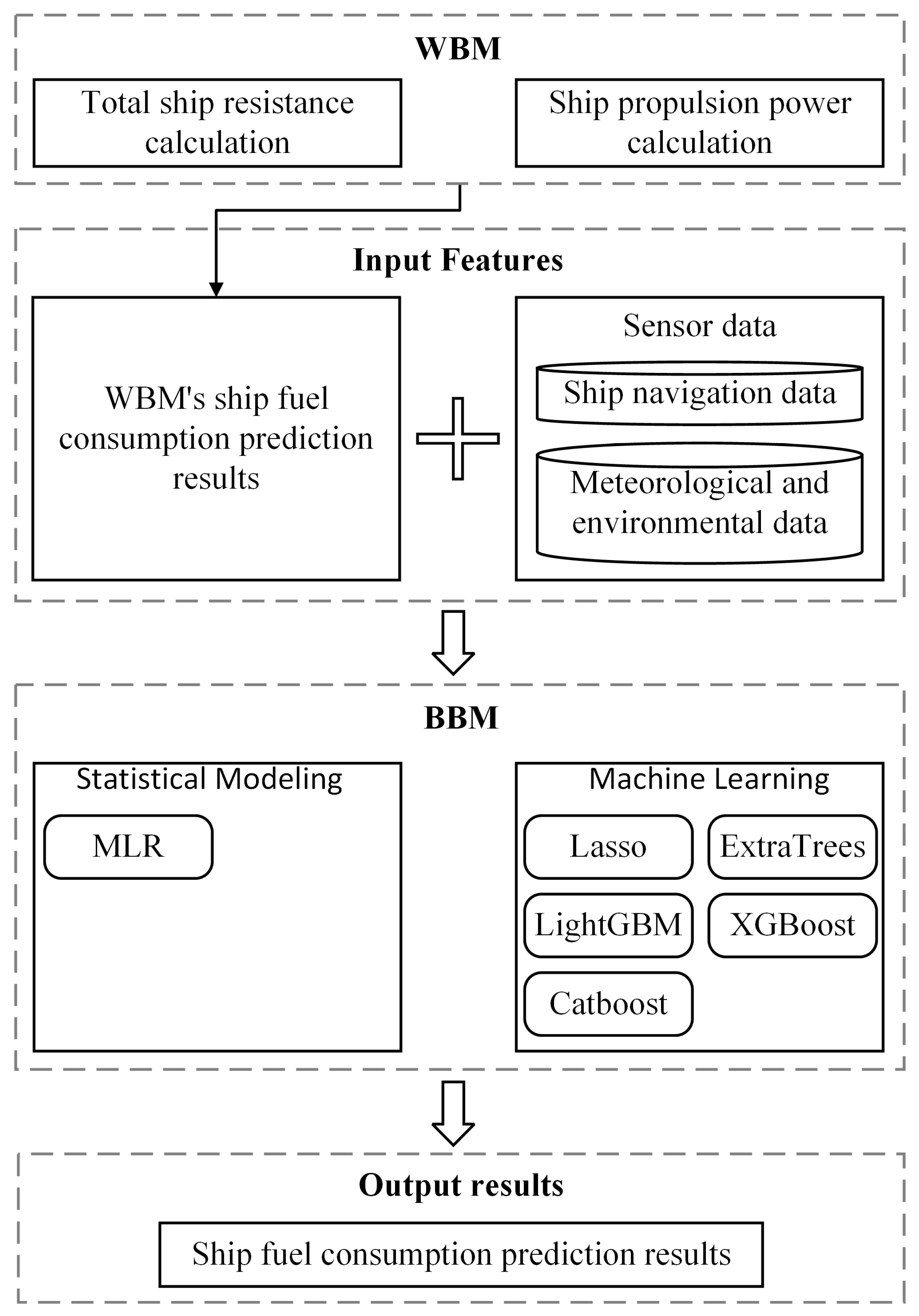
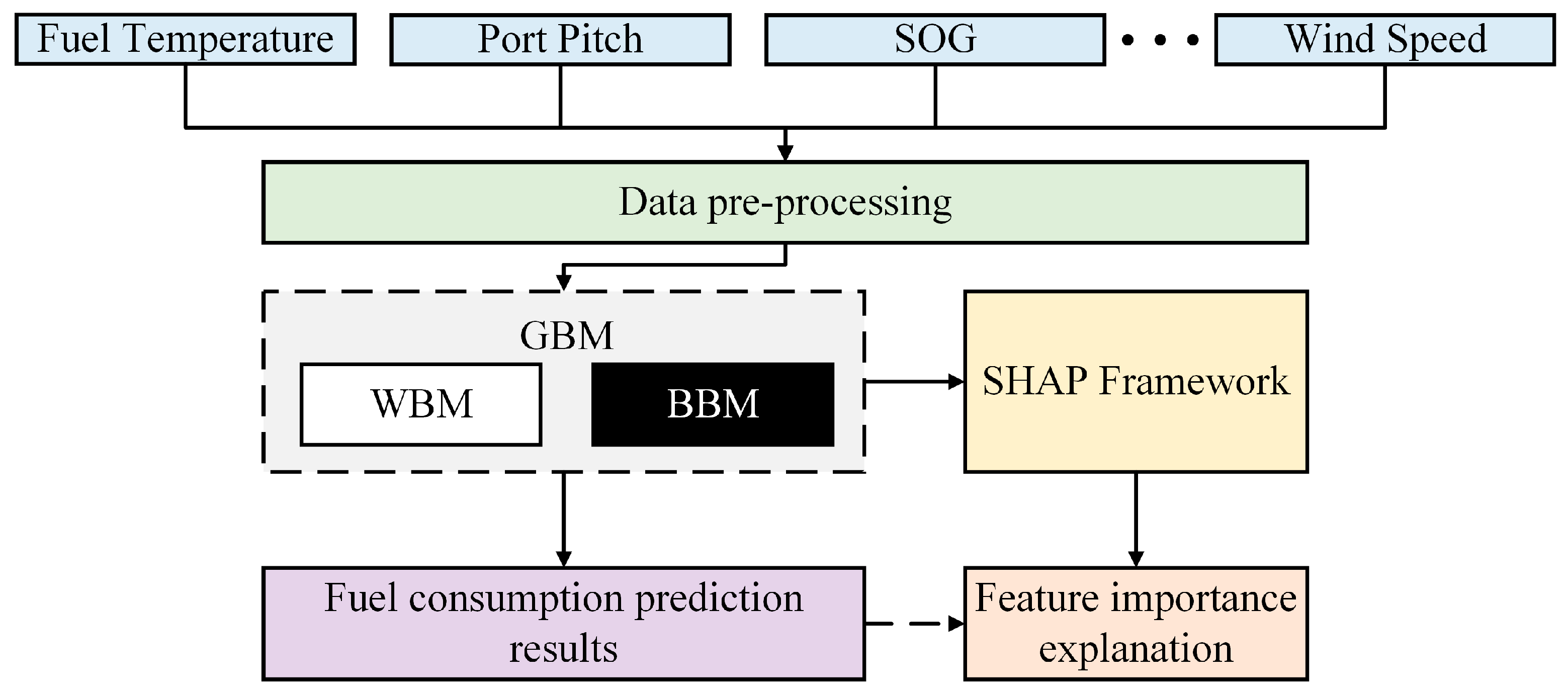
The purpose of this study is to propose a data-driven modeling method that can be widely used in ship fuel consumption prediction based on ship fuel consumption sensing monitoring data. The proposed predictive performance of the WBM, BBM, and GBM was verified on real data collected on various types of high-precision sensors installed on different parts of a ro-ro passenger ship. Another need of the model built is transparency or interpretability, i.e., the underlying and working process of the prediction model is interpretable and not only aiming at high prediction accuracy. Since BBMs and GBMs based on black box theory lack good interpretability, they cannot provide companies or maritime agencies with physically interpretable analysis of the impact of different influencing factors on ship fuel consumption, making it difficult for the technicians involved to trust the final prediction results. Therefore, this study introduces a framework of additive feature-based interpretation methods, SHAP, to improve the understanding of the prediction results of black box theory models. In addition, researchers can have redundant features in the selection of prediction model input features. The vast majority of information provided by redundant features is already represented by other features, and too many input features can increase the capital investment in data collection for ship companies, as well as significantly increase the memory storage requirements and computational costs for data analysis [21]. Regression prediction performance depends on the efficiency of the pattern between response and predictor variables, and redundant features that are highly correlated with each other also complicate prediction and affect the stability of predicted fuel consumption [22]. Therefore, this study further removes the redundant features from the input features with the help of the analysis results of SHAP. The main components of this study are shown in Figure 1, and the main contributions are as follows:
  • In this study, 19 multisource sensing data were preprocessed so that they could be used for ship fuel consumption prediction analysis;
  • In this study, a WBM based on the foundation of physical principles is established to convert the ship resistance calculated from the external environment and the energy transfer relationship between engine–propeller–ship into fuel consumption at a specific speed; secondly, six BBMs covering statistical models and machine learning models are established to map the relationship between multiple input features and fuel consumption. Finally, the GBM effectively combines the WBM and BBM models through a chaining strategy, which has better prediction performance and stability than the WBM and BBM, and obtains a ship fuel consumption prediction model suitable for practical engineering applications;
  • This study combines the high-performance GBM with the SHAP framework, solves the difficult problem of the poor interpretability of the underlying working principle of the model, quantitatively demonstrates the influence of input features on ship fuel consumption, and further validates the effectiveness of the WBM on GBM prediction performance improvement. On the other hand, based on the results of the importance analysis of input features, it provides an effective reference method for the selection of the best input features for ship fuel consumption prediction modeling, taking into account the prediction performance and input cost.

2. Material and Methodology

2.1. Data Description

The case ship used in this study is the Danish passenger ro-ro vessel MS Smyril, which operates on the route from Torshavn, the capital of the Faroe Islands, to Island Suduroy, with a one-way journey time of about 1 h 55 min and two to three round trips per day.
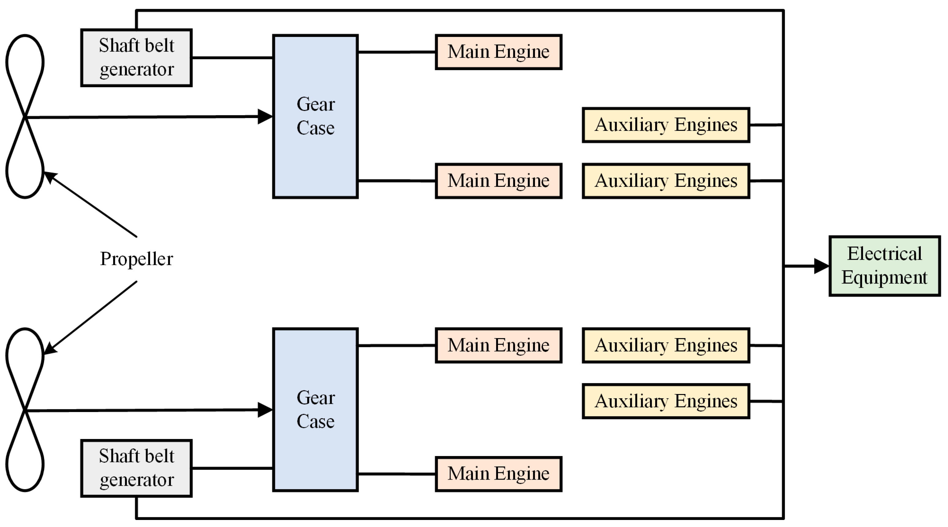
The MS Smyril has various sensors installed in different parts to collect various types of data during the operation of the ship and has published the operation data for 246 voyages from February to April 2010, with the main scale parameters of the ship obtained from Lloyd’s Register of Shipping (shown in Table 1). The ship’s power system is shown in Figure 2. The diesel main engine is a four-stroke MAN 32/40 type, which is connected to the shaft generator through a gearbox, and the four auxiliary engines together with the shaft generator provide power to the ship’s electrical system.
The MS Smyril has various sensors installed in different parts, and a total of 19 kinds of monitoring data, including the daily operation of the ship and the sea state environment during the ship’s voyage, were collected through the sensors, as shown in Table 2, and all data were collected during the voyage of the case ship.

2.2. Data Preprocessing

2.2.1. Missing Data Imputation

The accuracy of the data-driven ship fuel consumption prediction models is still strongly influenced by the quality of the data. Many factors during the voyage, including equipment stability and signal transmission, result in sensor systems collecting data that contain a large number of missing data points. The huge amount of sensing data can cause infinite accumulation and amplification of small errors in the prediction process, which greatly increases the uncertainty and accuracy of the calculation results. In the process of ship operation, the sensor system collects data often in the form of time series. In this study, a missing value is interpolated by the linear interpolation method [23], which is shown in Equation (1).
y = y 0 + ( y 1 y 0 ) t t 0 t 1 t 0
where y 0 and y 1 are the missing values of ship operating characteristics at moments t 0 and t 1 , respectively, and y denotes the missing values of ship operating characteristics at moment t ( t 0 , t 1 ) .

2.2.2. Data Standardization

The sensed data were preprocessed with Z-score normalization so that the data was transformed to have a distribution with a mean of 0 and a variance of 1. This avoids the high-value features from dominating the low-value features in the prediction process due to the different data magnitudes. The standardization Equations (2) and (3) are shown below:
σ = 1 N i = 1 N ( x i μ ) 2
Z - s c o r e = x i μ σ
where μ is the mean of the N sensor data samples and σ is the standard deviation of the N sensor data samples.

2.3. White Box Models

Quickness is one of the important hydrodynamic properties of a ship. Ship rapidity, which refers to the ability of a ship to maintain a certain speed of navigation by the thrusters absorbing energy from the main engine to form thrust to overcome resistance, includes both ship resistance and ship propulsion. The general approach to model the predicted fuel consumption of a ship’s white box is based on the application of the physical principle basis as well as the laws of fluid dynamics to calculate the results of the resistance encountered by the ship from different sources. By modeling the total drag conditions, it is possible to calculate the corresponding fuel consumption required to drive the ship at a given speed [10]. The model structure and parameters of the WBM have been determined from a priori knowledge and theoretical insights based on physical and hydrodynamic laws, shipbuilding principles, and computational hydrodynamic methods [24], and the ship model assumptions have been set according to the actual conditions of operation before the model is built, which means that the parameters inside the model cannot be adjusted during the ship’s voyage [25], and therefore are mainly applied in the initial stages of ship design and during sea trials.

2.3.1. Model Assumptions

The WBM proposed in this study uses the actual parameters of the ship under study and various assumptions of the model structure to parameter estimation to achieve the fuel consumption prediction for the ship with the following assumptions, shown below:
  • The ship is in a steady state underway. It is assumed that when the ship is sailing on a fixed course in a fixed area, the environmental condition is stable and the state of the ship keeps a steady state underway, i.e., the forces are in balance.
  • The speed is regulated by changing the propeller pitch, i.e., the engine speed is constant.
  • The seawater temperature is taken as the global average ocean temperature of 3.5 °C.
On the other hand, the WBM constructed in this paper is not specific to a particular ship type, and related workers can select the parameters we listed in the model construction according to the specific ship type to achieve the ship fuel consumption prediction, which ensures the generality.

2.3.2. Total Ship Resistance Model Considering Environmental Factors

In the actual navigation process, the ship will be subject to the resistance of both water and air media, so the total resistance of the ship can be divided into the water resistance of the underwater part and the air resistance of the water part. Therefore, this study further refines the ship resistance into five components: frictional resistance, residual resistance, attached resistance, air resistance, and wave accretion resistance.
The water resistance is further divided into two parts: hydrostatic resistance and wave resistance during navigation, which is influenced by the ship’s hull type and the roughness of the hull surface. Hydrostatic resistance includes bare hull resistance and appendage resistance, and appendage resistance refers to the additional resistance brought by the appendage above the bare hull of the ship in the flow field. In hydrostatic resistance, from the mechanism of resistance can be divided into frictional resistance, viscous pressure resistance, and emerging wave resistance, where viscous pressure resistance and emerging wave resistance are collectively referred as residual resistance. The ship movement process due to the viscous role of water will be subject to water viscous shear stress, wherein the combined force in the direction of movement is the hull friction resistance; viscous pressure resistance refers to the fluid viscosity and the formation of the boundary layer on the surface of the hull, and which causes the hull tail fluid flow separation to form a vortex to reduce the pressure difference between the hull tail so that the ship’s head and tail pressure difference is formed; wave resistance describes that the ship in the water will rise over the waves, resulting in the ship before and after the pressure distribution not being symmetrical, with the bow for the high-pressure area and the stern for the low-pressure area, so the role in the ship movement is in the opposite direction of the differential pressure force.
The resistance above the water surface mainly comes from the resistance of air to the hull superstructure, and the size of air resistance is related to the shape of the water part of the ship and the relative wind speed [26]. The resistance is increased by the wave action when the ship sails in the wind, and waves are wave resistance, which is influenced by the wave height, wave period, and wavelength of the waves [27].
In summary, the total ship resistance model constructed in this study is shown in Equation (4):
R t = R f + R r + R a p + R a + R a w
where R t is the total ship resistance, R f is the frictional resistance, R r is the residual resistance, R a p is the attached resistance, R a is the air resistance, and R a w is the wave acceleration resistance. The detailed description about the model of each drag component is shown in the first part of the supporting information. Detailed information about the calculation models for each resistance component are in the Appendix A Section.

2.3.3. Ship Propulsion Model

When the ship–machine–propeller is paired together, it forms an energy balance system. The propeller receives and converts energy to propel the ship; the energy balance between the propeller and the main engine means that, when the ship is sailing normally, the power issued by the main engine consuming fuel is driven by the shaft system to turn the propeller, and the thrust obtained is balanced with the resistance of the ship to ensure that the ship maintains a certain speed. When the ship is sailing at a constant speed, the main engine provides power to the ship, the gearbox and the drive shaft transmit the output power of the main engine to the propeller, and the propeller rotates to generate thrust to overcome the resistance of the ship during sailing, the main engine of the ship, the propeller, and the hull form a balanced system of energy, and this process is the ship–machine–propeller matching relationship. The acquisition of propeller thrust and torque can be theoretically calculated according to an empirical formula. According to the propeller working principle, its thrust calculation formula is shown in Equation (5):
T = K T ρ n p 2 D p 4
The propeller torque calculation formula is shown in Equation (6):
Q = K Q ρ n p 2 D p 5
where: K T is the thrust coefficient; K Q is the torque coefficient; ρ is the water density in kg / m 3 ; D p is the propeller diameter in m ; n p is the propeller speed in r / s . The thrust coefficient K T and the torque coefficient K Q can be calculated by the interpolation of the Wageningen B series plots.
The power from the main engine is transmitted to the propeller through the ship’s shaft system first, and the power obtained by the propeller is less than the power issued by the main engine of the ship due to the intermediate power transfer loss. In this power system, the main engine is the energy source which outputs the main engine power by consuming fuel. Then, the ship’s main engine power transmits the power to the propeller through the drive shaft system, and the power obtained by the propeller will be affected by the shaft system efficiency pair between the ship’s main engine and the propeller. The propeller generates thrust by rotating the acquired power, where the ratio of propulsive power transferred by the propeller to the acquired power is the product of the relative rotational efficiency and the propeller open water efficiency. Propulsion power is further transferred to the hull, and eventually, the hull gains effective power, where the ratio of the effective power gained by the hull to the propulsion power transferred by the propeller is the hull efficiency. The effective power of the hull is then converted into the final power to overcome the resistance of the hull, and the detailed information about calculation of the transfer efficiency in the ship propulsion system is shown in the Appendix B Section.

2.3.4. White Box Model of Ship Fuel Consumption

The host power can be deduced from the effective power according to the host power transfer relationship and the transfer efficiency between the parts, and thus the fuel consumption of the ship per unit of time can be derived, as shown in Figure 3.
Therefore, based on energy conservation theory, ship stress analysis, and transmission efficiency, the white box model of ship fuel consumption is shown in Equation (7):
b e = P M E g e
where b e is the host unit time fuel consumption, P M E is ship host power, and g e is the host fuel consumption rate, which can be obtained from the host technical specifications.
When the ship maintains a certain steady speed, i.e., uniform speed, it is known from Newton’s law of motion that the effective thrust T p produced by the propeller is equal to the total resistance R t of the ship:
T P = F P ( 1 t ) = R
The relationship between the effective power P e of the hull and the power P M E generated by the ship’s main engine is:
P M E = P e η H η P η R η S
P e = R t U
where η H , η P , η R , η S is the hull efficiency, open water efficiency, relative rotation rate, and shaft system efficiency, respectively.

2.4. Black Box Model

In recent years, with the accessibility of large amounts of data about ship energy efficiency collected from onboard sensors, machine learning techniques are becoming more mature in engineering applications. ML-based regression models are widely used in fuel prediction studies, and BBM models are more suitable for handling high-dimensional data compared to WBMs. As a result, a wider range of input features can be handled in the prediction of ship fuel, including ship navigation information, the surrounding ocean, and weather conditions. Thus, new data are accurately predicted based on the statistical pattern relationship between input features and ship fuel consumption established from the training set without requiring any prior knowledge about the system being modeled.
Ship fuel consumption black box models are data-driven models which are mainly divided into two categories. The first category is the BBM based on statistical modeling, and the widely used multiple linear regression (MLR) is used in this study. The second category is the BBM based on the ML algorithm, which does not require any a priori knowledge of ship performance and the model parameters are not physically meaningful and interpretable. This study is not intended to exhaust all ML models, but to cover the current ML algorithms that are widely adopted and stable in engineering, including the traditional ML algorithm Lasso (Least absolute shrinkage and selection operator). ExtraTrees (Extremely Randomized Trees) are based on the Bagging ensemble learning algorithm, and the algorithm flow is shown in Figure 4a. The XGBoost (eXtreme Gradient Boosting), LightGBM (Light Gradient Boosting Machine), and Catboost (Categorical Boosting) are based on the Boosting ensemble learning algorithm, and the algorithm flow is shown in Figure 4b. Ensemble learning algorithms provide better generalization and stability by effectively combining different models with unique characteristics to address the limitations of individual models. This study aims to find ML algorithms that are universally applicable to fuel consumption prediction, and the algorithms all use default hyperparameters.

2.4.1. Multiple Linear Regression

The basic principle of multiple linear regression [28] is to model the relationship between multiple independent variables using the least squares method. The general form of a multiple linear regression model is:
Y = β 0 + β 1 X 1 + β 2 X 2 + + β k X k + ε
where X i ( i = 1 , 2 , , k ) represents is the kth independent variable, β 0 represents the regression constant, β i represents the regression coefficient, and ε represents the random error term, which is the random error after removing the effect of the kth independent variables on Y . The regression coefficients in the above equation are estimated using the least square method.

2.4.2. Lasso

In 1996, Tibshirani [29] invented the Lasso regression approach, which regularizes the sum of absolute values of the regression coefficients by a penalty function. This method compresses the regression coefficients. The following optimization issues are resolved by the L1 parametric penalized least squares algorithm [22] known as Lasso:
w * = ( α , β ) = arg min ( i = 1 n ( y i α i X i β ) + λ β 1 )
where X i is the i-th independent variable, y i ( i = 1 , 2 , , n ) is the dependent variable, α is the constant term, β is the regression coefficient, and β 1 represents the L1 parametric, which indicates the compression strength of the coefficients. For hyperparameter λ ( 0 , ) , the larger the λ , the greater the penalty, and the fewer variables are retained in the model. As the value of λ decreases, the number of variables retained in the model starts to become larger.

2.4.3. ExtraTrees

Geurts et al. proposed ExtraTrees, a random forest-based system, in 2006 [30]. In contrast to random forests, which use random sampling to choose the sample set as the training set for each decision tree, in ExtraTrees, each decision tree uses the entire training set, which has a high utilization rate of training samples and can somewhat lessen the final prediction bias. This prevents random forests from not fully utilizing all of their samples. To guarantee structural variations between each decision tree, ExtraTrees incorporates more randomness into node splitting and potential similarity among decision trees. After N rounds of training, N decision trees with various topologies are produced, and the prediction outcomes of these diverse decision trees are then aggregated and averaged to provide model output h ¯ ( x ) .
h ¯ ( x ) = 1 N t = 1 N { h ( x , θ t ) }

2.4.4. XGBoost

In 2016, Chen et al. proposed an XGBoost algorithm based on GBDT (gradient-boosted decision tree) [31], which prevents overfitting by introducing second-order derivatives and regular terms with the objective function shown in Equation (12).
y ^ i = ϕ ( x i ) = K = 1 K f k ( x i ) ,   f k F
where F = { f ( x i ) = ω q ( x ) } ( q : m T , W = ( ω 1 , ω 2 , ω T ) T ) is the regression tree space. Each additional tree is equivalent to adding a new function to the model to fit the residuals of the last prediction, thus minimizing the canonical loss. Unlike the GBDT, XGBoost adds a regular term to the loss function as the objective function, which is shown in Equation (15).
O b j ( t ) = i = 1 N l ( y i , y ( t 1 ) + f t ( x i ) ) + Ω ( f t ) + c o n s t a n t
where l denotes the differentiable loss function that measures the difference between the predicted value y i and the straight real value y i , N is the number of samples, and Ω ( f ) represents the regular term of model complexity. To minimize O b j ( t ) , the model as a whole needs to be optimized. Using the Taylor expansion to fit the original objective function, a second-order Taylor expansion can be performed on the objective function, as shown in Equation (16).
f ( x + Δ x ) f ( x ) + f ( x ) Δ x + 1 2 f ( x ) Δ x 2
where the canonical terms are:
Ω ( f ) = γ T + 1 2 λ W 2
Ω ( f ) is the complexity of the tree. The lower the value, the simpler the tree structure. W represents the fraction of leaves and T represents the number of leaves, where L2 regularization is used.
After removing the constant term c o n s t a n t , the objective function is expressed as Equation (18):
O b j ( t ) = j = 1 T [ ( i I j g i ) W j + 1 2 ( i I j h i + λ ) W j 2 ] + γ T
The simplified objective function, Equation (19), is obtained by the leaf node traversal and further making G j = i I j g i , H i = i I j h i :
O b j ( t ) = j = 1 T [ G i W j + 1 2 ( H j + λ ) W j 2 ] + γ T
The weights of leaf node j will be calculated by deriving the objective function, transforming it to 0, and substituting it into Equation (19), resulting in the final result, as in Equation (20):
O b j * = 1 2 j = 1 T G j 2 H j + λ + γ T
In the next step, to find the best cut point of the leaf node and to determine the best construction of the tree, a greedy algorithm is used, as shown in Equation (21):
G a i n = 1 2 [ G L 2 H L + λ + G R 2 H R + λ ( G L + G R ) H L + H R + λ ] γ
G L 2 H L + λ is the score of the measure corresponding to the left subtree, G R 2 H R + λ is the score of the measure corresponding to the right subtree, and ( G L + G R ) H L + H R + λ is the score before the tree is disaggregated. γ is a penalty term to adjust the complexity of the tree. The pseudo code is shown below, as shown in Algorithm 1.
Algorithm 1: Exact Greedy Algorithm for Split Finding
Input :   I , instance   set   of   current   node Input :   d ,   dimension g a i n 0 G i I g i ,   H i I h i for   k = 1   to   m   do      G L 0 , H L 0      for   j   in   sorted ( I , b y   x j k )   do          G L G L + g i ,   H L H L + h i          G R G + G L ,   H R H + H L         score max ( s c o r e , G L 2 H L + λ + G R 2 H R + λ ( G L + G R ) H L + H R + λ )      end end output :   split   with   max   score

2.4.5. LightGBM

In 2017, Microsoft Research proposed the LightGBM model [32], which is an ensemble regression tree model based on gradient-boosting decision trees. LightGBM algorithm uses a Leaf-wise leaf growth strategy with depth restriction to search for the leaf with the largest splitting gain (usually the largest amount of data) from all existing leaves and then splits it cyclically and repeatedly compared with GBDT’s traversal of all data and XGBoost’s layer-by-layer splitting. The LightGBM algorithm sets a limit on the maximum depth of the leaf-wise to reduce the possibility of overfitting while maintaining high efficiency. It can directly support data parallelism and feature parallel learning, which greatly improves the speed of searching for the best segmentation point required.
In addition, LightGBM is a histogram-based decision tree algorithm. First, the continuous floating-point feature values are discretized into n integers and constructed as a histogram with the width equal to n. In the process of traversing the data, the discretized values are used as indexes, and the statistics are accumulated in the histogram and further traversed with the indexes of the histogram to search for the best segmentation points, thus speeding up the learning process and reducing memory consumption, as shown in Algorithm 2.
Algorithm 2: Histogram-based Algorithm
Input :   I , training   data ,   d :   max   depth Input :   m ,   feature   dimension n o d e S e t { 0 } tree   nodes   in   current   level r o w S e t { { 0 , 1 , 2 , } } data   indices   in   tree   nodes for   i = 1   to   d   do      for   n o d e   in   n o d e S e t   do          u s e R o w s r o w S e t [ n o d e ]          for   k = 1   to   m   do               H new   Histogram ( )               Build   histogram               for   j   in   u s e R o w s   do                   bin I . f [ k ] [ j ] . bin                   H [ bin ] . y H [ bin ] . y + I . y [ j ]                   H [ bin ] . n H [ bin ] . n + 1              Find   the   best   split   on   histogram   H                        Update   r o w S e t   and   n o d e S e t   according   to   the   best   spilt   points

2.4.6. Catboost

In 2017, the dominant Russian search engine Yandex proposed the Catboost algorithm [33], which, in contrast to LightGBM, automatically converts category-based features into numerical features by first performing statistical calculations on category-based features to determine how frequently a category feature occurs before adding hyperparameters to produce new numerical features. In order to extend the feature dimension by utilizing the connections between features, Catboost also incorporates category-based features.
Catboost uses a standard improvement to Greedy TS by adding a priori distribution terms to reduce the effect of noisy data on the data distribution, which is shown in Equation (22):
x k i = j = 1 p 1 [ x σ j , k x σ p , k ] Y σ j + a p j = 1 p 1 [ x σ j , k = x σ j , k ] + a
where p is the added prior term and a is usually a weighting factor greater than 0. For the regression problem, Catboost performs a random permutation of the dataset, and the prior term takes the mean of the dataset labels, effectively reducing the effect of noisy data on the distribution.
The conventional gradient boosting algorithm is replaced by Catboost and transformed into ordered boosting (OB), as shown in Algorithm 3. As a result of this algorithm’s capacity to successfully combat the noise points in the training set, gradient estimation bias is avoided. The issue of inescapable gradient bias in the iterative process is resolved, and the model’s generalizability is enhanced. Here is the pseudo code:
Algorithm 3: Ordered Boosting
Input :   { ( X k , Y k ) } k = 1 n   ordered   according   to ,   the   number   of   trees   I σ random   permutation   of   [ 1 , n ] M i 0   for   i = 1 n for   t 1   to   I   do      for   i 1   to   n   do          r i y i M σ ( i ) 1 ( x i ) ;      for   i 1   to   n   do          Δ M          L e a e n M o d e l ( ( x j , r j ) :          σ ( j ) i ) ;          M i M i + Δ M ; return   M n

2.5. Gray Box Model

The GBM is a combined WBM and BBM modeling approach that can be understood as using data-driven techniques to improve existing white box models with uncertain parameters or by adding black box components to the physical model output. In this study, a serial approach to the GBM construction strategy is used, in which the WBM precedes the BBM, and in which the WBM theory establishes the physical equilibrium equation between propulsion power and ship drag to predict fuel consumption. The fuel consumption predicted by the WBM is then fed into the BBM model as a new feature, and the BBM predicts the fuel consumption based on the a priori information given by the WBM and the navigation monitoring data collected by the sensors, at which point the black box is regarded as a regression model, and each run of the GBM requires the initial run of the WBM, as shown in Figure 5 [9]. The serial approach allows for combining the WBM with various types of BBM models and is more intuitive [34].
The initial dataset is the ship fuel consumption feature data X = { x 1 , x 2 , , x p } , X denotes the feature data involved in the white box model, and X denotes the feature data involved in the black box model, X X , X X . The WBM input is X and the output is the ship fuel consumption h W B M ( X ) . The BBM input is a function of X and the output is the ship fuel consumption h B B M ( X ) . The WBM fuel consumption is added to the BBM black box input dataset and updated to obtain the GBM input dataset of the gray box model of ship fuel consumption in tandem form as:
D G B M = [ X h W B M ( X ) ]
Based on this new dataset, the predicted values of the fuel consumption based on the gray box model are finally output by continuous training iterations based on the errors. From this, it can be seen that each run of the GBM requires an initial run of the WBM.

2.6. SHAP Framework

BBMs and GBMs containing BBMs are often complex, are trained in a completely data-driven manner, and while having high performance, the models often lack intuitive ship physical interpretability. In particular, the nonlinear prediction models constructed by tree-based ExtraTrees, XGBoost, LightGBM, and Catboost have the values of input features scattered among the branches and weights of each tree, and cannot measure the degree of influence of input influences on fuel consumption with a single equation relationship, which is not conducive to the identification of the importance of factors influencing fuel consumption on ships, and therefore difficult to be accepted by researchers in the shipping industry [35].
In 2017, Lundberg S et al. proposed a framework of additive feature interpretation methods based on SHAP [36]. SHAP is a method of calculating the Shapley value based on game theory, where each input feature is considered as a contributor, the contribution value of each feature is calculated, and the final prediction of the model is obtained by summing up the contribution value of each feature [37]. Compared with traditional feature importance methods (e.g., feature importance calculation methods such as random forests [34]), SHAP has better consistency to present the local and global interpretation of each predictor relative to the target variable. Each feature has a set of Shapley values that are used to calculate the local interpretability. Thus, the contribution of each feature of each sample to the fuel consumption prediction is well interpreted and also facilitates the researchers to analyze the reliability of the BBM and GBM models. The final global interpretability will be calculated by summing and averaging the Shapley values of all samples.
The feature importance of each feature i is calculated as shown in Equation (24):
ShapValues = S N \ { i } | S | ! ( M | S | 1 ) ! M ! [ f x ( S { i } ) f x ( S ) ]
where M is the number of input features, N is the set of all input features, and S is a set of nonzero feature indices. f x ( S ) = E [ f ( x ) | x s ] is the model’s prediction of the input x , where E [ f ( x ) | x s ] is the expected value of the function conditioned on a subset S of the input features, and a larger SHAP value indicates a larger contribution of the feature.

2.7. Model Evaluation Standards

To evaluate the effectiveness of the ship fuel consumption prediction model, two performance indicators are used: root mean square error (RMSE) and mean absolute error (MAE). Among them, RMSE is the evaluation of the degree of variation of the data and is the square root of the ratio of the square of the deviation of the observed value from the true value and the number of observations n. It is the most representative evaluation index in the regression model, especially for large data, as shown in Equation (25); MAE is the average of the absolute value of the deviation of all individual observations from the arithmetic mean, which better reflects the actual situation of the prediction value error, as shown in Equation (26). R2 is then a measure of the percentage change in the dependent variable in the regression model, which reflects the combined effect of the regression curve on the observed data points, as shown in Equation (27), where the closer R2 is to 1, the higher the predictive performance.
R M S E = 1 n i = 1 n ( y i y ^ i ) 2
M A E = 1 n i = 1 n | y i y ^ i |
R 2 = 1 i = 1 n ( y i y ^ i i ) 2 i = 1 n ( y i y ^ i ) 2
where y i is the predicted output value—predicted ship fuel consumption (L/h), and y ^ i is the target value—actual fuel consumption rate of the ship (L/h), while n is the number of samples in the dataset.

2.8. Cross-Validation

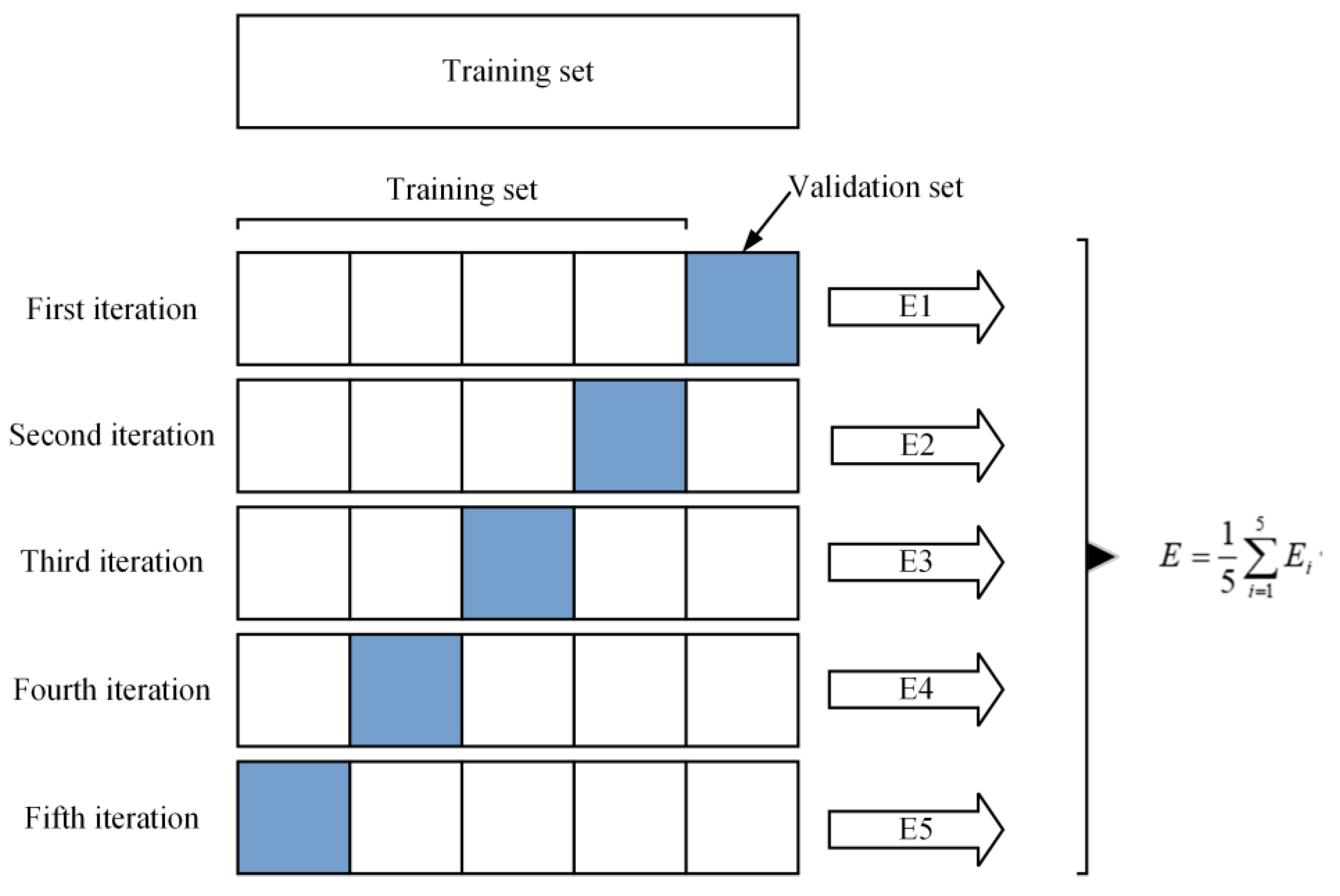
To further improve the accuracy and reliability of model evaluation, K-fold cross-validation is applied for training the model, and the main idea is to minimize any potential bias of random sampling of training and validation data subsets. The training set is divided into K equal-sized parts, with the K-1 part considered as the new training set and one part as the validation set. Eventually, K models will be trained and the average accuracy of the K models is taken to evaluate the model performance, and the value of K is usually set to 5, as shown in Figure 6. In addition, K-fold cross-validation can avoid the occurrence of overfitting to some extent, and the results are more convincing.

3. Results and Discussion

3.1. Predicted Results for WBM, BBM, and GBM

In this study, the monitoring data of the fuel-consumption-related ship status and environmental information were measured and recorded by sensors at the moments from 20:48:14 on 16 February 2010 to 21:35:36 on 2 March 2010 and were selected. However, there is some variation in the sensor sampling frequency due to the varying standards of the sensors. Therefore, these data must be preprocessed before they can be used to model the ship’s fuel consumption. Firstly, the time parameter of the sensor is used as a criterion to measure whether it is duplicated or not, and multiple identical data at the same time point can be considered as duplicated data and rejected. Secondly, the minimum common multiple (3 s) of each sensing data is used to unify the time granularity, which makes it possible to extract the features related to ship fuel consumption at the same time point, ensuring that sensor data with different sampling frequencies can be analyzed on the same time horizontal axis, and 403,800 complete data are obtained. Finally, the linear interpolation method in Section 2.2 is used to supplement the data acquisition process with some missing data due to factors, such as equipment stability and signal transmission, and the data are normalized by Equations (2) and (3) to avoid the influence of the magnitude.
The WBM established in Section 3.1 was used for validation, and the performance of the WBM was evaluated using the model evaluation metrics in Section 2.3, and the experimental results are shown in Table 3. The results show that the WBM does not show sufficient accuracy compared to the actual measurement results. The fact that the ship drag component in the model was treated separately, ignoring the effect of its interaction on the propulsion power, and that the effect of sea state (i.e., wind and waves) on the required propulsion power was not considered, is considered to be the source of large prediction error that exists in the model.
Next, the BBMs built by MLR and the Lasso, ExtraTrees, XGBoost, LightGBM, and Catboost algorithms were validated. This study does not aim to find a specific combination of hyperparameters for each type of ML algorithm based on experiments, so the default hyperparameters of each model from the six ML algorithms are simply used, as shown in Table 4. The model development environment for the study was implemented under Windows 11 Professional operating system using Python 3.7 programmed under Jupyter notebook software. The hardware configuration is a 12th Generation(R) Core(TM) i9-12900K 3.20 GHz processor, 64-bit operating system and 64.0 GB of RAM from Intel Corporation, USA, with the XGBoost model developed using XGBoost 1.6.1 library, the LightGBM model developed using LightGBM 3.3.2 library, the Catboost model developed using Catboost 1.0.6 library, and the rest of the models developed using Scikit-learn 1.1.1.
Before the BBM can make predictions, the model needs to be trained with a portion of the data so that the model learns the mapping relationship between fuel consumption and the influencing factors. Therefore, the dataset is divided here into a training set, which accounts for 70% of the original data, and a test set, which accounts for 30% of the original data. The training set is used for the BBM model training and the test set is used to evaluate the predictive performance of the model.
In order to ensure the robustness of the results to eliminate the error caused by randomness and the effect of data time dependence on model selection, this study first randomly splits the dataset into training and test sets five times. Thus, five random splits of the dataset required five model training sessions, resulting in five trained models (with the same type of ML algorithm). In addition, the K-fold cross-validation method in Section 2.8 is used in model training, where K is set to 5, and the process is as follows:
  • Randomly dividing the 70% training set into five parts without duplication;
  • Selecting one of them as the test set and the remaining four as the training set for model training, obtaining a model after training on the training set, testing it on the validation set with this model, and saving the evaluation metrics of the model;
  • Repeat step 2 five times (make sure each subset is given one chance to be the validation set);
  • The average of the five sets of test metrics is calculated as the final result of the model accuracy evaluation and used as the performance metrics of the model under the current five-fold cross-validation.
Finally, the average prediction performance of the five trained models (six BBM models based on different ML algorithms) on the 30% test set was used as the final result of the model evaluation, and the results were retained to three decimal places, as shown in Table 5.
Comparing Table 3 and Table 5, it can be found that both statistical-modeling-based and ML-based BBM models can achieve much higher prediction performance than the WBM by utilizing multiple input features compared to the WBM. Since the WBM is usually prebuilt, this means that the parameters inside the model cannot be adjusted during the ship’s voyage and some of the internal parameters are susceptible to environmental influences, leading to errors in the overall model [25]. From Table 5, it can be observed that there are some differences in the prediction performance of different BBMs. To build an accurate and reliable BBM, it is necessary to choose a suitable prediction algorithm, and the ensemble learning BBM shows better generalization ability, among which the prediction performance of Boosting-based XGboost, LightGBM, and Catboost BBMs are more excellent, especially the Catboost algorithm, with the RMSE and MAE of 47.394 L/h and 25.129 L/h, respectively, on the test set recommended to be applied to the actual fuel consumption prediction process and shows a better prediction performance than the other five BBM models.
Next, this study built the GBM based on Section 2.5 with the same training and test sets as those used for the BBM. Table 5 also shows the prediction results of the six GBMs, and it can be seen that, by using the prediction results of the white box model as prior knowledge, the prediction performance can be further improved on the original basis, and the effectiveness of the gray box model is verified. The enhancement of the prior knowledge provided by the WBM is larger for the two traditional linear regression models, MLR and Lasso, with the RMSE decreasing by 15.843 L/h and 8.597 L/h, respectively, and the MAE decreasing by 6.880 L/h and 4.90 L/h, respectively. However, the improvement is smaller for the models of Bagging and Boosting classes because the input information has been fully learned and the prior knowledge of the WBM only serves to correct some of the biases. Although the prediction accuracy of the WBM is lower, it can still give some prior knowledge to the BBM, which makes the GBM obtain a higher prediction accuracy than the BBM.
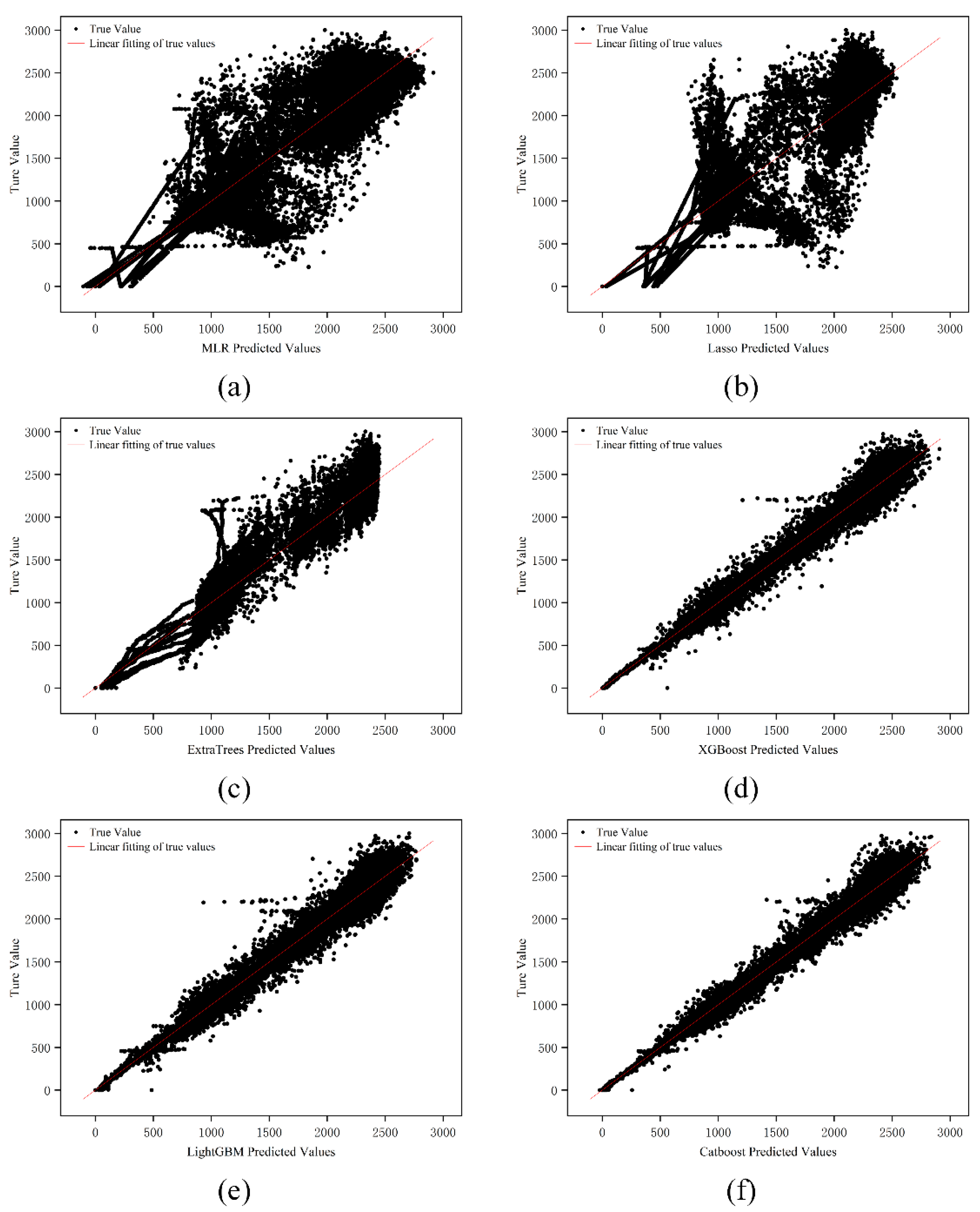
The prediction results of ship fuel consumption are the basis for the optimization of ship energy efficiency, and the choice of the prediction algorithm will directly affect the validity of the final prediction model. In order to more intuitively assess the consistency between the six GBM prediction values and the real value of fuel consumption values, the R2 score was calculated by Equation (27). Figure 7a–c depicts the fit of the predicted and true values of the GBM based on the MLR, Lasso, and ExtraTrees algorithms on the test dataset, and it can be clearly found that there are large deviations and the overall linear relationship is more ambiguous.
The GBM models based on the XGBoost, LightGBM, and Catboost algorithms, on the other hand, exhibit a significant linear relationship, as shown in Figure 7d–f, and can provide stable prediction results, with Catboost’s fit being more concentrated and having fewer sample points with larger deviations than LightGBM and XGBoost. In summary, the high R2 values of the GBM based on the Catboost algorithm indicate that the predicted values match well with the true values, proving that it has sufficient adaptability and accuracy to predict the fuel consumption of ships.
This study was compared with similar work using the same sensing data, and with the entire trip split, the RMSE for fuel consumption prediction using artificial neural networks (ANNs) and Gaussian processes (GPs) in the study of reference [38] was 69.1 L/h and 104 L/h, respectively, while the RMSE for the LightGBM, XGBoost, and Catboost algorithms for all six BBMs and GBMs in this study have lower RMSEs than their findings, especially the RMSE of the GBM based on the Catboost algorithm at 47.25 L/h, and this corresponds to a reduction in the RMSE of 46% and 119%, respectively, as shown in Figure 8.

3.2. Results of Model Explainability Analysis

Although the GBM has excellent computational performance characteristics, the complexity of the model is also increased, which is usually accompanied by poor model interpretability. SHAP utilizes the knowledge of game theory, i.e., the marginal diminishing effect of features, and is a logically rigorous feature interpretation method. Combining SHAP with GBM can quickly and precisely obtain the degree of importance of input influences and fuel consumption, which provides a basis for the precise optimization of ship energy efficiency in the future.
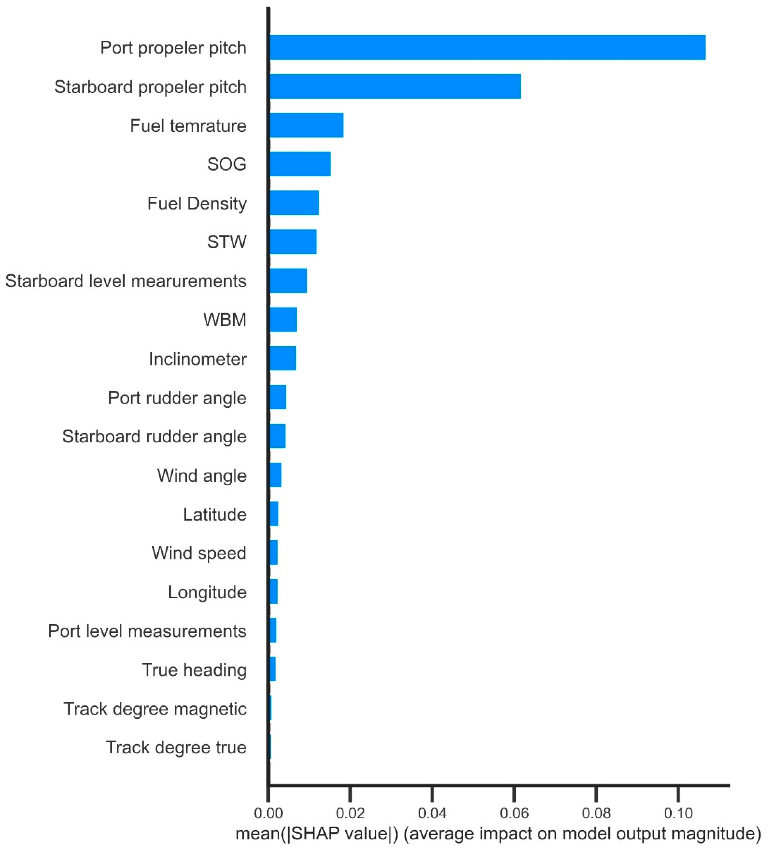
The importance results of nineteen input features of the GBM were obtained by SHAP, and only the top ten input features that have the greatest impact on the fuel consumption of the ship are listed in this section, as shown in Table 6. It can be found that the WBM is always one of the ten most important features of the GBM. This indicates that the GBM can effectively utilize the prior knowledge generated by the WBM during model training, explaining the reason why the prediction effect of the GBM is better than that of the BBM in Section 3. As the prediction accuracy increases, the feature’s importance gradually converges. The first three feature compositions of XGBoost, LightGBM, and Catboost, which have better prediction accuracy, are consistent, and the higher prediction accuracy indicates that the relationship between the GBM mining influence factors and fuel consumption is more accurate.
Therefore, the GBM based on the Catboost algorithm with the highest prediction accuracy is chosen here to analyze the factors affecting fuel consumption from a physical perspective, as shown in Figure 9, where the first five important influencing factors are mainly analyzed. Of these, port pitch and starboard pitch are the two most important factors, as they are the most direct indicators of the power used to move the vessel. The “thermal efficiency” of the engine in the best operating environment can be effectively converted into mechanical energy; that is, the proportion of power, combustion into thermal energy into kinetic energy, the fuel temperature is low, and the engine combustion work generated by heat energy will be more conducted into the air, thus affecting fuel consumption. On the other hand, the fuel temperature will directly affect the fuel density. The physical and chemical properties of the fuel show that the lower the temperature of the oil body, the higher the density, and the smaller the volume, the higher the viscosity. Conversely, the higher the temperature of the oil body, the density will continue to become smaller and the viscosity will continue to decrease and the volume will continue to increase. The fuel injection volume of the engine is determined by the plunger volume. When the fuel density increases, the mass of fuel injected into the cylinder will increase, and it will lead to poor atomization of fuel, causing the incomplete combustion of the engine, and the fuel consumption rate will rise; on the contrary, when the fuel density becomes smaller, the fuel consumption rate of the engine will decrease, which is the reason why there is a strong correlation between fuel temperature, fuel density, and the fuel consumption of the ship [39,40]. Ship speed (SOG) is identified as the fourth most important variable for prediction, which is in line with the general conclusion in the relevant literature, where sailing speed is the most important determinant of ship fuel, of which the cubic law is particularly well-known [14,41]. It can also be found that the sea state information of wind direction and wind speed have less influence on ship fuel consumption, ranking twelfth and fourteenth in importance among the nineteen input features, and all six GBMs do not include them among the ten most relevant features, which creates some deviation from the expectation of the correlation hypothesis. This problem is effectively explained in a related study by Soares and Coraddu, in which they argue that the design phase of the shipboard automation system takes into account the time-domain variation of sea state conditions to ensure a constant speed profile by varying the pitch setting and fuel consumption rate. Therefore, under their assumptions, the two input features of port pitch and starboard pitch, which are most important for fuel consumption effects, already include information on the effects of environmental factors on fuel consumption [34,42]. The results show that the combination of SHAP and GBM models can effectively help researchers understand the prediction results and provide a quantifiable reference for increasing ship energy efficiency and reducing emissions through operational optimization.
After obtaining the total importance ranking of the input variables affecting ship fuel consumption by combining SHAP with the Catboost-based GBM model, this study wanted to know which influencing factors should be involved in the GBM to obtain accurate prediction results. This is due to the fact that, as the number of input features increases in the prediction process, the cost of sensor data acquisition as well as computational analysis increases, but the improvement in prediction performance may be of diminishing marginal benefit due to the existence of information redundancy among the input features, where a large amount of information of some features is already contained in other features of the input. To find the best input features to meet the application requirements, this study builds GBM models based on the Catboost algorithm with nineteen different input sets, where the first input set contains only the top-ranked features, while the second input set contains the top two features, and then the third input set covers the top three features, and so on, as shown in Appendix C. For these 19 GBMs, 70% of the data samples are still used for training the model, and the remaining 30% are used for validating the model.
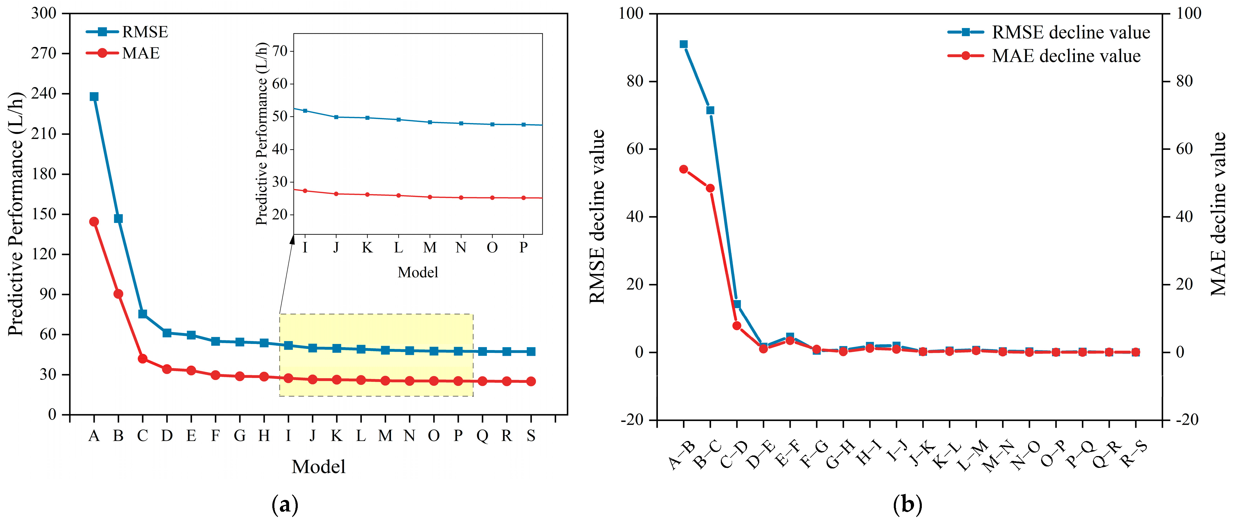
The prediction performance and generalization ability of the 19 trained GBM models were evaluated on the test set, and the prediction results are shown in Table 7 where the RMSE values and MAE gradually decreased by adding the input features one-by-one. For the four most important input variables, the prediction performance was significantly improved by gradually introducing port pitch, starboard pitch, fuel temperature, and the SOG. From model A to model D, the RMSE and MAE decreased by 74.27% and 76.40%, respectively. The changes in the RMSE and MAE among the 19 GBMs shown in Figure 10a are generally consistent with the ranking of the importance of the input variables shown in Figure 8. When a fifth influencing factor, fuel density, is added to model D, the improvement in intermodel prediction performance is significantly smaller than that of the first four models. The amount of change in intermodel prediction performance shown in Figure 10b shows that, when the characteristic wind speed is added to model M, the improvement in prediction performance based on the RMSE and MAE decreases significantly and is constant at a lower level. Therefore, it can be concluded that the best features for predicting ship fuel consumption are the set of input influences corresponding to model M. Continuing to add input features has a very limited improvement in prediction performance, and the RMSE and MAE between predicted and observed values only increase by 2.21% and 1.76% compared to model S, which contains all input features, but reduces the cost of collecting and computing six features.
Based on the results of this study, shipping companies and maritime organizations can select the type of sensors to be installed to maximize the benefits by considering the prediction accuracy, data acquisition, and calculation costs that are required in engineering applications.

4. Conclusions

In this study, the MS Smyril passenger roll-on/roll-off vessel was used as the research object. Based on the sensing data to obtain the ship’s characteristics and environmental factors, including the SOG, latitude and longitude, longitudinal inclination, wind, fuel density, heading, and other nineteen influencing factors, three ship fuel consumption prediction models, the WBM, BBM, and GBM, were established to map out the fuel consumption per unit time and the law. The prediction performance of the three types of models is compared horizontally, and the prediction performance of the BBM and GBM models based on different algorithmic principles is compared vertically to determine the best model to be applied to ship fuel consumption prediction. The SHAP method is also used to analyze the importance of the input features affecting ship fuel consumption from a global perspective, which solves the problem of the poor interpretability of the GBM. In addition, the model prediction performance under different subsets of input features is compared based on the importance ranking results of SHAP to determine the best input features for predicting ship fuel consumption. The following conclusions can be drawn:
  • In this study, the WBM, BBM, and GBM based on six different ML algorithms were established and tested on the sensor data from a passenger roll-on/roll-off vessel. The experimental results show that the prediction error of the WBM is much higher than that of the BBM and GBM and cannot be effectively used for the prediction of ship fuel consumption during actual ship operation. The ensemble learning algorithms based on Boosting, especially Catboost, show the best prediction performance, with RMSE values below 50 L/h on the test dataset. The GBM makes further improvement in prediction accuracy through the prior knowledge of the WBM, which can meet the demand of ship fuel consumption prediction. In practical engineering applications, companies only need to integrate the GBM model based on the Catboost algorithm into the fuel consumption prediction system to achieve accurate fuel consumption prediction.
  • This paper introduces the SHAP framework combined with the GBM based on the Catboost algorithm to provide a method that can accurately analyze the relative importance of different influencing factors on fuel consumption. The experiment verified the improved effect of the prior knowledge of the WBM on the predictive performance of the GBM model and additionally found that the four most important input factors affecting fuel consumption were port pitch, port pitch, fuel temperature, and the SOG.
  • Nineteen GBMs based on different input features were established according to the feature importance ranking provided by SHAP. Based on the prediction evaluation index, the best input influences were selected from the 19 GBMs by considering the prediction accuracy, data collection cost, and computation cost, which can predict the fuel consumption of a ship with fewer input features while ensuring a certain prediction accuracy, and provide a reference for sensor-based ship fuel prediction. It provides a reference for the selection of input features in prediction of sensor-based ship fuel.
It is worth noting that the SHAP-based GBM model proposed in this paper still needs further research in the future to make the model work better in practical engineering applications. On the one hand, we should consider trying to incorporate more high-quality input influences (e.g., ship maintenance records, etc.) to continuously improve the stability of the model prediction performance and expand its application scope. On the other hand, the modeling approach proposed in this study is not specific to a particular ship type and aims to establish a unified ship fuel consumption prediction model constructed by combining high-performance sensing data that can be universally applied, so that relevant researchers concerned can choose the arrangement of appropriate sensor equipment and model structure assumptions to realize fuel consumption prediction of ships in conjunction with actual conditions. The prediction performance of the model has been confirmed in a specific case. By randomly dividing the original data into five training and test sets, it is also further demonstrated that the proposed model is not affected by data randomness and time dependence, and more data can be collected from different voyages or ships in the future to further verify the generality of the model and improve the ship fuel consumption prediction model and the interpretable framework to achieve the best results of this study. Therefore, the proposed model can provide a reference for the IMO and shipping companies to address the environmental sustainability of shipping.
Author Contributions

Conceptualization, Y.Z.; methodology, J.Y.; software, Y.M.; validation, J.Z.; formal analysis, J.Z.; investigation, Y.M.; resources, H.K.; data curation, Y.M.; writing—original draft preparation, Y.M. and J.Y.; writing—review and editing, Y.Z. and J.Z.; visualization, Y.M.; supervision, Y.Z.; project administration, J.Y.; funding acquisition, H.K. All authors have read and agreed to the published version of the manuscript.

Funding

The work was supported in part by the National Natural Science Foundation of China (grant numbers 72072017, 71902016, 71831002) and the Natural Science Foundation of Liaoning Province of China (grant number 2022-MS-162).

Institutional Review Board Statement

Not applicable.

Informed Consent Statement

Not applicable.

Data Availability Statement

The sensing data of the MS Smyril passenger roll-on/roll-off vessel used in this study were obtained from the publicly available database established by Petersen et al. http://cogsys.imm.dtu.dk/propulsionmodelling/data.html (accessed on 6 January 2023).

Acknowledgments

The authors would like to thank anonymous reviewers and editors.

Conflicts of Interest

The authors declare no conflict of interest.

Appendix A

The detail calculation processes of each resistance component are explained here.
  • Frictional resistance
Frictional resistance A is the frictional force formed on the hull surface by the tangential stress caused by the viscosity of the water; the combined force formed by the frictional force in each direction in the direction of the ship’s motion is the overall frictional resistance. Considering the hull surface is difficult to express with the display function, it is difficult to calculate the hull frictional resistance. Therefore, Fu Rude put forward the concept of “equivalent plate”, assuming that the ship’s frictional resistance is equivalent to its role in the same rate of movement and length, and the wet surface area is the same smooth plate. However, in the actual modeling process, the surface of the ship is not absolutely smooth, and will become “rough” in different degrees due to uneven painting, welding seams, marine life adhesion, etc., making the actual frictional resistance greater than the frictional resistance of the smooth hull. Usually, “hull surface roughness allowance” is used to express this effect. So, the hull frictional resistance can be estimated by the frictional force of “quite flat plate”, plus the increase of frictional resistance caused by the roughness of hull surface, as shown in Equation (A1):
R f = ( C f + Δ C f ) 1 2 ρ U 2 S
where C f is the equivalent to flat plate friction drag coefficient; Δ C f is the surface roughness allowance coefficient; ρ is the mass density of fluid (water) in kg/m3; U is the ship’s speed in m/s; S is the wet surface area of the hull in m2.
The calculation of the frictional drag coefficient of the equivalent flat plate in Equation (A1) is based on the most commonly used formula for calculating the frictional drag coefficient, as shown in Equation (A2), which was presented at the 8th International Towing Tank Conference (ITTC) in 1957 by analyzing the drag test results of geometrically similar ship models.
C f = 0.075 ( lg Re 2 ) 2
Re in Equation (A2) is the Reynolds coefficient, which is defined as (A3):
Re = U L v
where L is the length of the ship in m and v is the kinematic viscosity coefficient of the fluid (in this case water) in m2/s. The kinematic viscosity coefficients of seawater at different temperatures are shown specifically in Table A1.
Table A1. Kinematic viscosity coefficient of seawater at different temperatures.
Temperature (°C) Kinematic   Viscosity   ( × 10 6 m 2 s ) Temperature (°C) Kinematic   Viscosity   ( × 10 6 m 2 s )
51.5650151.1907
61.5191161.1617
71.4775171.1338
81.4339181.1071
91.3942191.0813
101.3563201.0565
111.3202211.0327
121.2587221.0098
131.2527230.9878
141.2211240.9664
The values in Equation (A1) can be referred to the following Table A2 subsidy coefficients for different captains.
Table A2. Kinematic viscosity coefficient of seawater at different temperatures.
Length of Ship (m) Δ C f × 10 3
50~1500.35~0.4
150~2100.2
210~2600.1
260~3000
300~350−0.1
350~450−0.25
The wet surface area in Equation (A1) is calculated as shown in Equation (A4) below:
S = L × d × ( 2 + B 2 d ) 1.625 C B
where d is the draft in m; B is the ship type width in m; C B is the squareness factor. The ship square factor can be derived from Equation (A5):
C B = L · B · d
where is the drainage volume in m3.
In summary, the frictional resistance of the ship can be found, as shown in Equation (A6):
R f = [ 0.075 ( lg U L v 2 ) 2 + Δ C f ] · ρ U 2 L 2 B d ( 4 d + B ) 6.5 L B d 4
2.
Residual resistance
The formula for calculating the residual resistance to the ship is shown in Equation (A7).
R r = C r 1 2 ρ U 2 S
The relationship between the frictional drag coefficient and the residual drag coefficient is shown in Equation (A8).
C r = ( 25.02 F n 3 7.752 F n 2 + 1.246 F n + 0.2568 ) C f
where F n is the Fourier number, which can be calculated by Equation (A9).
F n = U g L
where U is the speed, g is the acceleration of gravity, and L is the captain.
3.
Attachment resistance
The ship is equipped with a rudder, axle wrapper, and other appendages protruding from the hull, and the resistance increment to these appendages is the appendage resistance. When calculating the appendage resistance, in addition to calculating the resistance of each appendage, also to calculate the interference resistance between each appendage and the hull, so the accurate appendage resistance calculation is difficult; in general, one can use the empirical formula or model test to determine it, where the empirical formula has the following (A10) calculation method:
R a p = C a p ( R f + R r )
where C a p is the attachment coefficient and the value can be referred to the attachment resistance coefficient of different types of ships in Table A3.
Table A3. Reference value of captain’s Subsidy under different circumstances.
Additional EquipmentSingle Paddle Boats (%)Twin Paddle Boats (%)
Paddle Shaft Package Holder--2.5
Bilge Keel3.02.5
Rudder--2.0
Total3.07.0
4.
Air resistance
In the navigable environment, the wind comes from different directions and varies. For the description of wind class, the Beaufort wind class (Table A4) is used internationally, and the international common wind class classification table used in a wide range of life studies.
Table A4. Reference value of captain’s Subsidy under different circumstances.
Wind LevelTypem/sSpecifications
0Calm0.0~0.2Sea surface smooth and mirror-like
1Light Air0.3~1.5Scaly ripples, no foam crests
2Light Breeze1.6~3.3Small wavelets, crests glassy, no breaking
3Gentle Breeze3.4~5.4Large wavelets, crests begin to break, scattered whitecaps
4Moderate Breeze5.5~7.9Small waves, 1–4 ft., becoming longer, numerous whitecaps
5Fresh Breeze8.0~10.7Moderate waves, 4–8 ft, taking longer form, many whitecaps, some spray
6Strong Breeze10.8~13.8Larger waves, 8–13 ft, whitecaps common, more spray
7Near Gale13.9~17.1Sea heaps up, waves 13–19 ft, white foam streaks off breakers
8Gale17.2~20.7Moderately high (18–25 ft) waves of greater length, edges of crests begin to break into spindrift, foam blown in streaks
9Severe Gale20.8~24.4High waves (23–32 ft), sea begins to roll, dense streaks of foam, spray may reduce visibility
10Storm24.5~28.4Very high waves (29–41 ft) with overhanging crests, sea white with densely blown foam, heavy rolling, lowered visibility
11Violent Storm28.5~32.6Exceptionally high (37–52 ft) waves, foam patches cover sea, visibility more reduced
The wind will affect the hull above the water layer, and the resistance generated by the interaction between the ship and the air in the part above the water line during navigation is the air resistance. The air resistance is mainly related to the ship’s relative wind speed and the hull’s shape above the waterline. However, compared with other components of the resistance, the air resistance to the ship’s role is smaller, and the size of the air resistance R a is calculated as shown in the Formula (A11):
R a = 1 2 C a ρ a A t v a 2
where C a is defined as the air resistance coefficient; ρ a is defined as the mass density of air, usually taken as ρ a = 1.226   kg / m 3 ; A t is defined as the projected area of the cross-section of the part of the ship above the water surface; v a is defined as the relative speed of the ship and the air (the vector sum of the speed of the ship and the wind speed along the direction of the ship’s navigation).
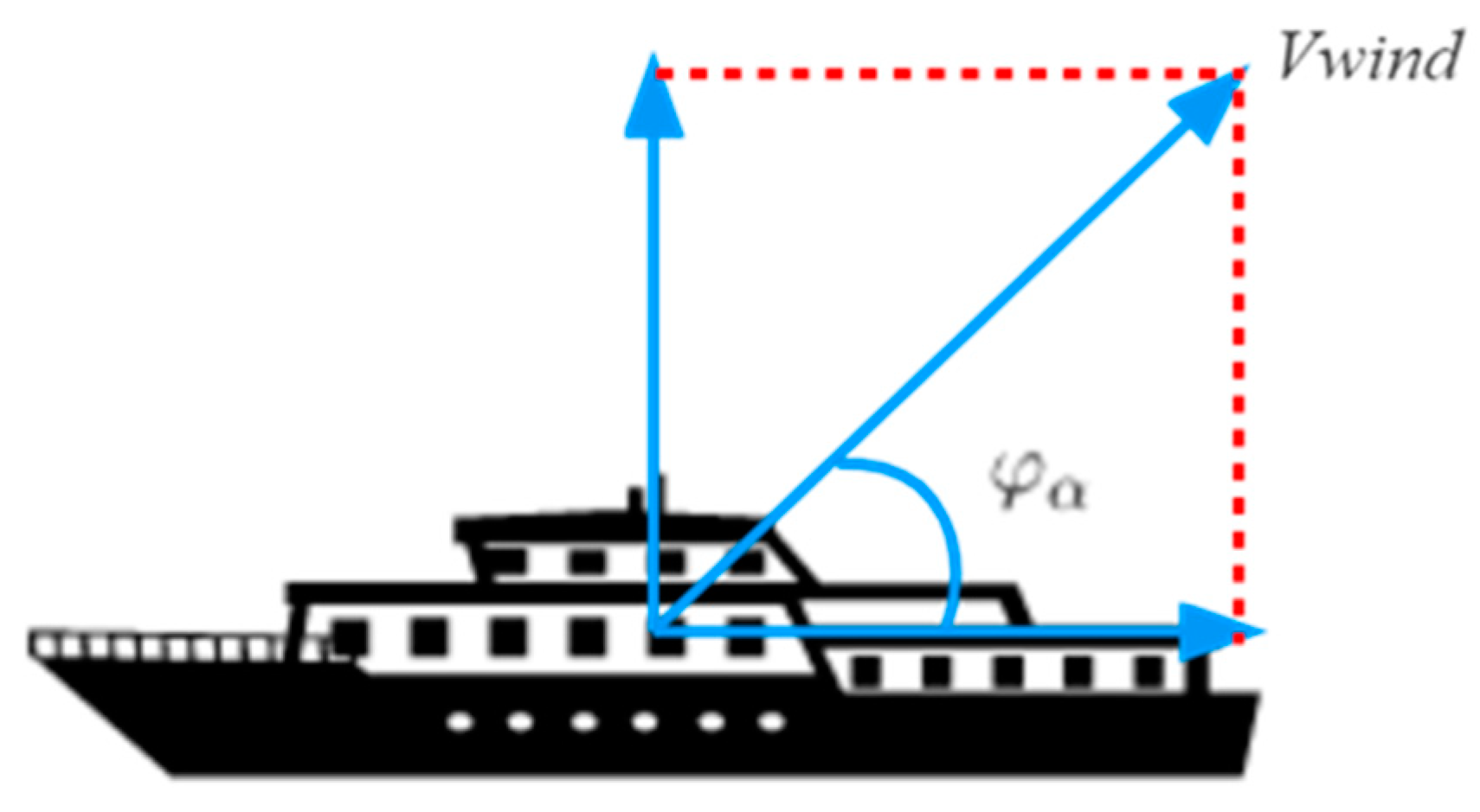
Combined with the ship navigation wind action diagram, the wind speed v w i n d is decomposed and its angle φ α with the ship’s forward direction is the relative wind angle. The relative velocity of the ship and the wind is shown in Figure A1, which is calculated as Equation (A12):
v a = U + v w i n d cos φ α
Figure A1. This is a figure. Schemes follow the same formatting.
Jmse 11 01059 g0a1
Air resistance coefficient According to the wind tunnel experiment statistics (Table A5), the general passenger ship takes 0.09, the cargo ship takes 0.10, and the fishing ship takes 0.04.
Table A5. Air drag coefficient of different types of ships.
Ship Type Average   Value   of   Air   Resistance   Coefficient   ( × 10 3 )
General Cargo Ships0.10
Bulk Carrier0.08
Fishing Boats0.04
Oil Tanker0.08
Passenger Ship0.09
Ferry0.10
Container Ship (no container on deck)0.08
Container Ship (with containers on deck)0.10
5.
Wave Incremental Resistance
The increase in resistance of the ship’s hull when sailing in waves relative to the resistance when sailing in still water makes the ship operate in complex sea conditions without a significant speed reduction. The principle of wave resistance increase is very complicated; when the wind acts on the water where the ship is running, the sea floor (coast) is affected by such seismic waves, and the sea level will form a periodic change in height, thus generating waves. The wave increment resistance is usually considered in the reserve power when the ship is designed, and the reserve power percentage is generally taken. For a ship under certain wind and wave sea conditions, the increment of its average effective power has the empirical Equation (A13):
Δ P = 4.594 ( 2 ξ w + 0.152 ) 2 C B L / B B
where ξ w is the wave height. The wave increase resistance is given by the power definition equation P = R v .
R a w = Δ P U = 4.594 ( 2 ξ w + 0.152 ) 2 C B L / B B U

Appendix B

This section shows the detailed calculation process of the transfer efficiency of each part of the ship propulsion system.
  • Open water efficiency
The thrust coefficient K T and torque coefficient K Q , as the propeller’s geometric parameters, reflect the propeller’s hydrodynamic performance. Without considering the effect of high waves, K T and K Q depend only on the propeller’s inlet speed coefficient J , which is calculated as shown in Equation (A15):
J = h p D p
where h p is the propeller process in m; D p is the propeller diameter in m. The propeller process, i.e., the distance the propeller rotates for one week to advance along the shaft, is shown in Equation (A16):
h p = v p n p D p
For the propeller open water efficiency η p , that is, the actual propeller work power and the ratio of the received power, by definition, the calculation process can be shown in Equation (A17).
η p = T v p Q 2 π n p
The above propeller open water characteristics are only the propeller operating characteristics under ideal conditions, where the interaction between the ship and the propeller will also affect the propeller operating characteristics, so other factors affecting the propeller propulsion efficiency need to be considered; at the same time, the rotation of the propeller increases the resistance of the ship, resulting in the propeller-generated thrust in addition to offset the resistance generated by the movement of the hull, but also need to offset the additional resistance generated by its rotation, so to calculate the effective thrust of the propeller on the hull, it is also necessary to calculate the thrust reduction factor.
2.
Shaft system efficiency
The power required by the propeller is transmitted from the ship’s main engine through a series of transmission devices according to the corresponding transmission efficiency; then, the total transmission efficiency between the ship’s main engine and the propeller via the transmission shaft system is the shaft system efficiency η s . Therefore, the relationship between the ship’s main engine power and the power received by the propeller can be expressed by the Equation (A18):
η s = P P P M E
3.
Relative rotational efficiency
When a ship is moving forward, the surrounding water flow is impacted by it and creates a companion current. The presence of the hull will cause a gap between the propeller feed speed and the ship’s speed, thus destroying the uniformity of the water flow at the propeller disc.
The presence of a companion current will produce a significant difference in the thrust or torque of the same propeller in the open water and aft. The ratio of thrust Q 0 from the open water propeller to thrust Q B from the aft propeller, when producing the same thrust at the same speed, is the relative rotation rate η R , as shown in Equation (A19):
η R = Q B Q 0
The companion flow fraction ω is shown in Equation (A20):
ω = V S V P V S = 1 V P V S
where V P is the propeller feed speed; V S is the ship speed.
When ship model tests are not possible, the accompanying flow coefficient can be estimated using empirical formulas. Two empirical formula estimation methods are given below:
  • Taylor’s formula (for transport vessels):
For single-propeller vessels:
ω = 0.5 C B 0.05
For double-propeller ships:
ω = 0.55 C B 0.20
  • Hankescher formula
For single-propeller standard merchant ships:
ω = 0.70 C P 0.18
For single-propeller fishing ships:
ω = 0.77 C P 0.28
For twin-propeller standard fishing ships:
ω = 0.70 C P 0.3
where C P is the rhombic coefficient.
4.
Hull efficiency
Similarly, the propeller motion has a corresponding effect on the moving hull, which is mainly reflected in the reduction of pressure in the rear part of the ship due to the suction effect of the propeller when the propeller is running behind the ship and the resulting increase of resistance. To overcome this part of the resistance increase, the thrust T from the propeller is not fully used to overcome the hull resistance R to propel the ship; that is, the thrust reduction.
The companion current and thrust reduction represent the interaction between the hull and the propeller, and the joint effect of both and the propulsion efficiency is reflected in the hull efficiency η H . The defining equation for hull efficiency (A26) shows that
η H = 1 t 1 ω
where t is the thrust derating factor, and the thrust derating factor t is calculated as shown in Equation (A27):
t = Δ F F p = F p T p F p = 1 T p F p
where Δ F denotes the thrust reduction; F P is the thrust generated by the propeller; T P is the effective thrust generated by the propeller.
When model testing is not possible, the thrust reduction fraction can also be estimated using empirical formulas. Two empirical formulas for estimating the thrust reduction fraction are listed below.
  • Hankescher formula
For single-propeller standard merchant ships:
t = 0.50 C P 0.12
For single-propeller fishing ships:
t = 0.70 C P 0.30
For twin-propeller standard merchant ships:
t = 0.50 C P 0.18
  • Shang-He formula
For single propeller ships:
t = k ω
where the coefficient k is determined by the form of the rudder:
  • k = 0.50 ~ 0.70 , for those equipped with streamlined or reactive rudders;
  • k = 0.70 ~ 0.90 , for double-plate rudders with square rudder posts;
  • k = 0.90 ~ 1.05 , for those equipped with a single-board rudder.
For twin-propeller ships with shaft mounts:
t = 0.70 ω + 0.06
For twin-propeller ships with shaft wrapped frames:
t = 0.25 ω + 0.14

Appendix C

Table A6. Nineteen models based on different sets of inputs.
ModelInput Influencing Factors
APort propeller pitch
BPort propeller pitch, Starboard propeller pitch
CPort propeller pitch, Starboard propeller pitch, Fuel temperature
DPort propeller pitch, Starboard propeller pitch, Fuel temperature, SOG
EPort propeller pitch, Starboard propeller pitch, Fuel temperature, SOG, Fuel density
FPort propeller pitch, Starboard propeller pitch, Fuel temperature, SOG, Fuel density, STW
GPort propeller pitch, Starboard propeller pitch, Fuel temperature, SOG, Fuel density, STW, Starboard level measurements
HPort propeller pitch, Starboard propeller pitch, Fuel temperature, SOG, Fuel density, STW, Starboard level measurements, WBM
IPort propeller pitch, Starboard propeller pitch, Fuel temperature, SOG, Fuel density, STW, Starboard level measurements, WBM, Inclinometer
JPort propeller pitch, Starboard propeller pitch, Fuel temperature, SOG, Fuel density, STW, Starboard level measurements, WBM, Inclinometer, Port rudder angle
KPort propeller pitch, Starboard propeller pitch, Fuel temperature, SOG, Fuel density, STW, Starboard level measurements, WBM, Inclinometer, Port rudder angle, Starboard rudder angle
LPort propeller pitch, Starboard propeller pitch, Fuel temperature, SOG, Fuel density, STW, Starboard level measurements, WBM, Inclinometer, Port rudder angle, Starboard rudder angle, Wind angle
MPort propeller pitch, Starboard propeller pitch, Fuel temperature, SOG, Fuel density, STW, Starboard level measurements, WBM, Inclinometer, Port rudder angle, Starboard rudder angle, Wind angle, Latitude
NPort propeller pitch, Starboard propeller pitch, Fuel temperature, SOG, Fuel density, STW, Starboard level measurements, WBM, Inclinometer, Port rudder angle, Starboard rudder angle, Wind angle, Latitude, Wind speed
OPort propeller pitch, Starboard propeller pitch, Fuel temperature, SOG, Fuel density, STW, Starboard level measurements, WBM, Inclinometer, Port rudder angle, Starboard rudder angle, Wind angle, Latitude, Wind speed, Longitude
PPort propeller pitch, Starboard propeller pitch, Fuel temperature, SOG, Fuel density, STW, Starboard level measurements, WBM, Inclinometer, Port rudder angle, Starboard rudder angle, Wind angle, Latitude, Wind speed, Longitude, Port level measurements
QPort propeller pitch, Starboard propeller pitch, Fuel temperature, SOG, Fuel density, STW, Starboard level measurements, WBM, Inclinometer, Port rudder angle, Starboard rudder angle, Wind angle, Latitude, Wind speed, Longitude, Port level measurements, True heading
RPort propeller pitch, Starboard propeller pitch, Fuel temperature, SOG, Fuel density, STW, Starboard level measurements, WBM, Inclinometer, Port rudder angle, Starboard rudder angle, Wind angle, Latitude, Wind speed, Longitude, Port level measurements, True heading, Track degree magnetic
SPort propeller pitch, Starboard propeller pitch, Fuel temperature, SOG, Fuel density, STW, Starboard level measurements, WBM, Inclinometer, Port rudder angle, Starboard rudder angle, Wind angle, Latitude, Wind speed, Longitude, Port level measurements, True heading, Track degree magnetic, Track degree true

References

  1. Christiansen, M.; Fagerholt, K.; Ronen, D. Ship Routing and Scheduling: Status and Perspectives. Transp. Sci. 2004, 38, 1–120. [Google Scholar] [CrossRef]
  2. Axel, M.; Joakim, K.; Abdalla, M. Port call optimization and CO2-emissions savings–Estimating feasible potential in tramp shipping. Marit. Transp. Res. 2022, 3, 100054. [Google Scholar]
  3. Xiaohe, L.; Yuquan, D.; Yanyu, C.; Son, N.; Wei, Z.; Alessandro, S.; Zhuo, S. Data fusion and machine learning for ship fuel efficiency modeling: Part I–Voyage report data and meteorological data. Commun. Transp. Res. 2022, 2, 100074. [Google Scholar]
  4. Gholizadeh, A.; Madani, S.; Saneinia, S. A geoeconomic and geopolitical review of Gwadar Port on belt and road initiative. Marit. Bus. Rev. 2020; ahead-of-print. [Google Scholar]
  5. Öztürk, O.B.; Başar, E. Multiple linear regression analysis and artificial neural networks based decision support system for energy efficiency in shipping. Ocean Eng. 2022, 243, 110209. [Google Scholar] [CrossRef]
  6. Yuquan, D.; Yanyu, C.; Xiaohe, L.; Alessandro, S.; Zhuo, S. Data fusion and machine learning for ship fuel efficiency modeling: Part III–Sensor data and meteorological data. Commun. Transp. Res. 2022, 2, 100073. [Google Scholar]
  7. Theocharis, D.; Rodrigues, V.S.; Pettit, S.; Haider, J. Feasibility of the Northern Sea Route: The role of distance, fuel prices, ice breaking fees and ship size for the product tanker market. Transp. Res. Part E 2019, 129, 111–135. [Google Scholar] [CrossRef]
  8. Wan, Z.; El Makhloufi, A.; Chen, Y.; Tang, J. Decarbonizing the international shipping industry: Solutions and policy recommendations. Mar. Pollut. Bull. 2018, 126, 428–435. [Google Scholar] [CrossRef] [PubMed]
  9. Leifsson, L.Þ.; Sævarsdóttir, H.; Sigurðsson, S.Þ.; Vésteinsson, A. Grey-box modeling of an ocean vessel for operational optimization. Simul. Model. Pract. Theory 2008, 16, 923–932. [Google Scholar] [CrossRef]
  10. Haranen, M.; Pakkanen, P.; Kariranta, R.; Salo, J. White, Grey and Black-Box Modelling in Ship Performance Evaluation. In Proceedings of the Hull Performance and Insight Conference 2016, Castello di Pavone, Italy, 13–15 April 2016. [Google Scholar]
  11. Li, X.; Sun, B.; Guo, C.; Du, W.; Li, Y. Speed optimization of a container ship on a given route considering voluntary speed loss and emissions. Appl. Ocean. Res. 2020, 94, 101995. [Google Scholar] [CrossRef]
  12. Kuntal, S.; Murthy, B.V.; Abhisek, U. Modeling and Real-Time Scheduling of DC Platform Supply Vessel for Fuel Efficient Operation. IEEE Trans. Transp. Electrif. 2017, 3, 762–778. [Google Scholar]
  13. Wang, K.; Yan, X.; Yuan, Y.; Li, F. Real-time optimization of ship energy efficiency based on the prediction technology of working condition. Transp. Res. Part D 2016, 46, 81–93. [Google Scholar] [CrossRef]
  14. Ryder, S.C.; Chappell, D. Optimal speed and ship size for the liner trades. Marit. Policy Manag. 1980, 7, 55–57. [Google Scholar] [CrossRef]
  15. Lepore, A.; Palumbo, B.; Capezza, C. Analysis of profiles for monitoring of modern ship performance via partial least squares methods. Qual. Reliab. Eng. Int. 2018, 34, 1424–1436. [Google Scholar] [CrossRef]
  16. Erto, P.; Lepore, A.; Palumbo, B.; Vitiello, L. A Procedure for Predicting and Controlling the Ship Fuel Consumption: Its Implementation and Test. Qual. Reliab. Eng. Int. 2015, 31, 1177–1184. [Google Scholar] [CrossRef]
  17. Petersen; Winther; Jacobsen. A Machine-Learning Approach to Predict Main Energy Consumption under Realistic Operational Conditions. Ship Technol. Res. 2012, 59, 64–72. [Google Scholar] [CrossRef]
  18. Chaal, M. Ship Operational Performance Modelling for Voyage Optimization through Fuel Consumption Minimization. Master’s Thesis, World Maritime University, Malmö, Sweden, 2018. [Google Scholar]
  19. Yang, L.; Chen, G.; Rytter, N.G.M.; Zhao, J.; Yang, D. A genetic algorithm-based grey-box model for ship fuel consumption prediction towards sustainable shipping. Ann. Oper. Res. 2019, 1–27. [Google Scholar] [CrossRef]
  20. Coraddu, A.; Oneto, L.; Anguita, D.; Baldi, F. Ship efficiency forecast based on sensors data collection: Improving numerical models through data analytics. In Proceedings of the Oceans, Genova, Italy, 18–21 May 2015. [Google Scholar]
  21. Kim, Y.; Kim, S.B. Collinear groupwise feature selection via discrete fusion group regression. Pattern Recognit. 2018, 83, 1–13. [Google Scholar] [CrossRef]
  22. Wang, S.; Ji, B.; Zhao, J.; Liu, W.; Xu, T. Predicting ship fuel consumption based on LASSO regression. Transp. Res. Part D 2017, 65, 817–824. [Google Scholar] [CrossRef]
  23. Meijering, E. A chronology of interpolation: From ancient astronomy to modern signal and image processing. Proc. IEEE 2002, 90, 319–342. [Google Scholar] [CrossRef]
  24. Ran, Y.; Wang, S.; Psaraftis, H.N. Data analytics for fuel consumption management in maritime transportation: Status and perspectives. Transp. Res. Part E 2021, 155, 102489. [Google Scholar]
  25. Ailong, F.; Jian, Y.; Liu, Y.; Da, W.; Nikola, V. A review of ship fuel consumption models. Ocean. Eng. 2022, 264, 112405. [Google Scholar]
  26. Luo, S.; Ma, N.; Hirakawa, Y. Evaluation of resistance increase and speed loss of a ship in wind and waves. J. Ocean. Eng. Sci. 2016, 1, 212–218. [Google Scholar] [CrossRef]
  27. Ke, Y.; Wenyang, D.; Limin, H.; Peixin, Z.; Shan, M. A prediction method for ship added resistance based on symbiosis of data-driven and physics-based models. Ocean. Eng. 2022, 260, 112012. [Google Scholar]
  28. Farag, Y.B.A.; Ölçer, A.I. The development of a ship performance model in varying operating conditions based on ANN and regression techniques. Ocean. Eng. 2020, 198, 106972. [Google Scholar] [CrossRef]
  29. Robert, T. Regression Shrinkage and Selection Via the Lasso. J. R. Stat. Soc. Ser. B 2018, 58, 267–288. [Google Scholar]
  30. Geurts, P.; Ernst, D.; Wehenkel, L. Extremely randomized trees. Mach. Learn. 2006, 63, 3–42. [Google Scholar] [CrossRef]
  31. Chen, T.; Guestrin, C. XGBoost: A Scalable Tree Boosting System. In Proceedings of the 22nd ACM SIGKDD International Conference on Knowledge Discovery and Data Mining, San Francisco, CA, USA, 13–17 August 2016. [Google Scholar]
  32. Qi, M. LightGBM: A Highly Efficient Gradient Boosting Decision Tree. In Proceedings of the Neural Information Processing Systems, Long Beach, CA, USA, 4–9 December 2017. [Google Scholar]
  33. Prokhorenkova, L.; Gusev, G.; Vorobev, A.; Dorogush, A.V.; Gulin, A. CatBoost: Unbiased boosting with categorical features. In Proceedings of the Advances in Neural Information Processing Systems, Long Beach, CA, USA, 4–9 December 2017. [Google Scholar]
  34. Coraddu, A.; Oneto, L.; Baldi, F.; Anguita, D. Vessels fuel consumption forecast and trim optimisation: A data analytics perspective. Ocean. Eng. 2017, 130, 351–370. [Google Scholar] [CrossRef]
  35. Lundberg, S.M.; Nair, B.; Vavilala, M.S.; Horibe, M.; Eisses, M.J.; Adams, T.; Liston, D.E.; Low, D.K.-W.; Newman, S.-F.; Kim, J.; et al. Explainable machine-learning predictions for the prevention of hypoxaemia during surgery. Nat. Biomed. Eng. 2018, 2, 749–760. [Google Scholar] [CrossRef]
  36. Lundberg, S.; Lee, S.I. A Unified Approach to Interpreting Model Predictions. In Proceedings of the Advances in Neural Information Processing Systems, Long Beach, CA, USA, 4–9 December 2017. [Google Scholar]
  37. Parsa, A.B.; Movahedi, A.; Taghipour, H.; Derrible, S.; Mohammadian, A.K. Toward safer highways, application of XGBoost and SHAP for real-time accident detection and feature analysis. Accid. Anal. Prev. 2020, 136, 105405. [Google Scholar] [CrossRef]
  38. Petersen, J.P.; Jacobsen, D.J.; Winther, O. Statistical modelling for ship propulsion efficiency. J. Mar. Sci. Technol. 2012, 17, 30–39. [Google Scholar] [CrossRef]
  39. Gong, C. Study of Fuel Temperature Effects on Fuel Injection, Combustion, and Emissions of Direct-Injection Diesel Engines. J. Eng. Gas Turbines Power 2009, 131, 022802. [Google Scholar]
  40. Mekonen, M.W.; Sahoo, N. Combined effects of fuel and intake air preheating for improving diesel engine operating parameters running with biodiesel blends. J. Renew. Sustain. Energy 2018, 10, 043103. [Google Scholar] [CrossRef]
  41. Adland, R.; Cariou, P.; Wolff, F.-C. Optimal ship speed and the cubic law revisited: Empirical evidence from an oil tanker fleet. Transp. Res. Part E 2020, 140, 101972. [Google Scholar] [CrossRef]
  42. Figari, M.; Soares, C.G. Fuel consumption and exhaust emissions reduction by dynamic propeller pitch control. In Analysis and Design of Marine Structures; CRC Press: Boca Raton, FL, USA, 2009; pp. 567–574. [Google Scholar]
Figure 1. Constituent framework for interpretable ship fuel consumption prediction.
Jmse 11 01059 g001
Figure 2. Smyril power system.
Jmse 11 01059 g002
Figure 3. Schematic diagram of the structure of the WBM.
Jmse 11 01059 g003
Figure 4. (a) Algorithm flow chart of bagging ensemble learning; (b) Flowchart of algorithm for boosting ensemble learning.
Jmse 11 01059 g004
Figure 5. GBM’s structural process framework.
Jmse 11 01059 g005
Figure 6. Diagram about cross validation.
Jmse 11 01059 g006
Figure 7. The results of the predicted and true values of six GBM models based on different ML algorithms on the test set: (a) MLR model (R2 = 0.887), (b) Lasso model (R2 = 0.858), (c) ExtraTree (R2 = 0.952), (d) XGBoost (R2 = 0.994), (e) LightGBM (R2 = 0.993), and (f) Catboost (R2 = 0.995).
Jmse 11 01059 g007
Figure 8. Comparison of the ship fuel consumption performance of the model proposed in this study with models from other references. The blue model is the prediction performance of the model built in this study, and the orange model is the prediction performance of the proposed model.
Jmse 11 01059 g008
Figure 9. Importance of the input features of the gray box model obtained in the SHAP framework.
Jmse 11 01059 g009
Figure 10. (a) Trend of 19 GBMs prediction performance based on different input sets; (b) The amount of change in prediction performance among 19 GBMs based on different input sets.
Jmse 11 01059 g010
Table 1. Hull main scale parameters.
ParametersValuesParametersValues
Ship Length135.00 mMain Engine ModelMAN Energy Solution 7L32/40
Length Between Perpendiculars123.00 mMain Engine Bore/Stroke320 mm × 400 mm
Molded Breadth22.70 mMain Power14,000 mkw × 750 rpm
Molded Depth8.10 mNumber of Auxiliary Engines4
Net Tons3801 tAuxiliary Engines Bore/Stroke160 mm × 240 mm
Deadweight Ton2067 dwtAuxiliary Power2640 mkw × 1200 rpm
Designed Draft5.6 mNumber of Axle Belt Generators2
Design Speed21.00 ktsInstalled Power13,440 Kw
Number of Main Engines4IMO No.9,275,218
Table 2. Nineteen types of monitoring data collected by sensors during the course of the route.
Sailing ParametersUnitsSailing ParametersUnits
Fuel TemperatureCPort Rudder−10–10 V
Fuel Densitykg/LSpeed Over Ground (SOG)Kn
Fuel Volume Flow RateL/sStarboard Pitch−10–10 V
InclinometerdegreesStarboard Rudder−10–10 V
Latitude Track Degree Magneticdegrees
Port Water LevelmTrack Degree Truedegrees
Starboard Water LevelmTrue Headingdegrees
Longitude Wind Angledegrees
Speed Through Water (STW)knWind Speedm/s
Port Pitch−10–10 V
Table 3. WBM performance indicators for predicting fuel consumption.
Fuel ConsumptionRMSR (L/h)MAE (L/h)
WBM925.79851.28
Table 4. The set of hyperparameters of 5 ML algorithms.
ML AlgorithmHyperparameter Set
LassoAlpha: 0.01
ExtraTreesCriterion = MSE; Max Depth: 6
XGBoostNumber of Iterations: 100; Max Depth: 6; Learning Rate: 0.1
LightGBMNumber of Iterations: 100; Boosting type: GBDT; Learning Rate: 0.1; Max Depth: −1; Drop Rate: 0.1
CatboostIterations: 500; Loss Function: Logloss; Learning Rate: 0.03; Max Depth: 6
Table 5. Predicted performance metrics of the BBM and GBM on the test set built using different machine learning algorithms in terms of fuel consumption.
Machine Learning AlgorithmsRMSEMAE
BBMMLR244.832151.942
Lasso264.852183.179
ExtraTrees149.706101.120
XGboost50.13327.374
LightGBM56.03731.368
Catboost47.39425.192
GBMMLR228.989145.062
Lasso256.255178.279
ExtraTrees148.806101.099
XGboost49.98927.208
LightGBM55.85031.071
Catboost47.25324.984
Table 6. Prediction results of the six GBMs on the test set.
RankMLRLassoExtraTreesXGBoostLightGBMCatboost
1WBMSTWPort PitchPort PitchPort PitchPort Pitch
2Fuel TemperatureWBMStarboard PitchStarboard PitchStarboard PitchStarboard Pitch
3Port PitchFuel TemperatureFuel TemperatureFuel TemperatureFuel TemperatureFuel Temperature
4Fuel DensityStarboard PitchSTWFuel DensityFuel DensitySOG
5InclinometerPort RudderSOGInclinometerInclinometerFuel Density
6SOGTrue HeadingFuel DensitySTWSOGSTW
7True HeadingStarboard RudderWBMSOGSTWStarboard Water Level
8Starboard RudderStarboard Water LevelPort RudderStarboard Water LevelStarboard Water LevelWBM
9Port RudderInclinometerInclinometerStarboard RudderWBMInclinometer
10Wind SpeedSOGStarboard RudderWBMPort RudderPort Rudder
Table 7. Prediction performance of 19 GBMs based on different input sets.
ModelRMSE (L/h)MAE (L/h)
A237.888144.486
B146.88090.410
C75.42041.962
D61.19334.096
E59.55533.095
F54.88929.642
G54.40028.746
H53.70828.516
I51.82927.349
J49.87426.435
K49.66626.230
L49.09325.934
M48.31925.434
N47.96625.290
O47.62825.258
P47.55625.211
Q47.32925.168
R47.28425.078
S47.25324.984
Disclaimer/Publisher’s Note: The statements, opinions and data contained in all publications are solely those of the individual author(s) and contributor(s) and not of MDPI and/or the editor(s). MDPI and/or the editor(s) disclaim responsibility for any injury to people or property resulting from any ideas, methods, instructions or products referred to in the content.