Research on Trajectory Tracking Control of Underwater Vehicle Manipulator System Based on Model-Free Adaptive Control Method

Abstract

In order to improve the trajectory tracking accuracy of an Underwater Vehicle Manipulator System (UVMS) under uncertain disturbance conditions of ocean current, a Model-free Adaptive Control (MFAC) method was used. Combined with Radial Basis Function Neural Networks (RBFNN), the RBFNN-MFAC method is proposed to improve the performance of the controller. A hydrodynamic model of UVMS was defined in the commercial software, Fluent, to calculate hydrodynamics disturbance, and the mechanism of the dynamic model of UVMS was defined in the commercial software, Adams, to simulate the motion of UVMS. The trajectory tracking performance with various control schemes, including PID (Proportional Integral Derivative), MFAC and RBFNN-MFAC, were analyzed with the Adams and Simulink joint simulation model. The results show that the position tracking accuracy and the speed tracking accuracy with the MFAC control scheme were 68.1% and 81.0% better, respectively, than those with PID control scheme. The position tracking accuracy and the speed tracking accuracy with the RBFNN-MFAC control scheme were 66.3% and 43.1% better, respectively, than those with the MFAC control scheme. The MFAC control scheme and the RBFNN-MFAC control scheme proposed in this paper exhibit good trajectory tracking performance without the precise dynamic model of UVMS, which is of great importance to applications in engineering.

1. Introduction

Underwater Vehicle Manipulator Systems (UVMSs) are important for ocean exploration and have been widely used in offshore oil production [1], marine aquaculture [2], underwater asset inspection [3] among other applications.

A UVMS is composed of two subsystems, the underwater vehicle and the underwater manipulator [4]. The kinematics and coupling effect between the underwater vehicle and manipulator are intrinsic factors affecting the performance of a UVMS. Wang et al. [5] proposed a new redundancy resolution method to address the motion coordination problem between the underwater vehicle and underwater manipulator of the UVMS that consists of a fuzzy logic component and a multitasks weighted gradient projection method component. Considering the effect of hydrodynamic force, Ambar et al. [6] proposed a resolved acceleration control (RAC) method to control a dual-arm UVMS and achieved coordinated control between the vehicle and the two robotic arms. Tang et al. [7] developed a control framework consisting of online motion planning, multitask kinematic control, dynamic feedforward compensation, and adaptive parameter undulatory control for a UVMS, in which the influence on the vehicle induced by the manipulator was described as a dynamic feedforward compensation signal to reduce undesired waggle. Han et al. [8] designed a fuzzy decoupling controller (FDC) using a fuzzy algorithm (FA) to adaptively tune the gain matrix of the error function (EF), and adopted off-diagonal elements to exploit dynamic coupling among the degrees of freedom of the subsystem and the dynamic coupling between the two subsystems of a UVMS. Barbalata et al. [9] developed a decoupled approach based on the separated control of the two subsystems and a coupled approach treating the two subsystems as a single system, which both used a parallel position/force control structure with sliding mode controllers and incorporated a mathematical model of the system. The two methods were able to compensate the coupling effects between the vehicle and the manipulator. However, the above research did not take the effect of ocean current disturbance on the UVMS into consideration, and the results were difficult for use in engineering practice.

An underwater vehicle is a six degrees of freedom subsystem, and the manipulator has extra degrees of freedom, which makes the UVMS a redundant degree of freedom system. Considering these redundancy characteristics, Haugaløkken et al. [10] designed three different kinematic control schemes, a decoupled kinematic control scheme, a full kinematic control scheme and a full modified kinematic control scheme, which were all suitable for controlling UVMS using kinematic control. Han et al. [11] proposed a performance index for redundancy resolution, as the distance from the center of gravity to the center of buoyancy of the UVMS, to reduce restoring moments and control efforts, and further proposed a nonlinear optimal controller with a disturbance observer for tracking control of the UVMS. Santhakumar [12] proposed a tracking control scheme to perform power efficient trajectory based on the kinematics redundant nature of UVMS. However, ocean current disturbance is highly random, and the above research did not fully consider adaptive ability to t random disturbance.

The trajectory tracking accuracy of the manipulator endpoint is the key to determine the applicable working conditions and the working efficiency of a UVMS. El-Ferik et al. [13] proposed an adaptive control scheme of an artificial potential field formation-based approach to address the problem of fleet containment for a UVMS under the leader-follower strategy with direct topology. Wang et al. [14] have proposed a closed-loop control system based on binocular vision to achieve the autonomous operation. Furthermore, Wang et al. [15] proposed a nonsingular terminal sliding mode control (NTSMC) method based on time delay estimation (TDE), and conducted a pool experiment using a seven degrees of freedom UVMS to obtain an end effector control precision of 0.067 m. However, the above research did not consider ocean current disturbance either. In addition, the control schemes required strong calculation capability, and it was difficult to achieve online real-time control of the UVMS.

The uncertain disturbance of ocean current is an extrinsic factor affecting the performance of a UVMS. To address the unknown hydrodynamic forces and moments created by the variable ocean current, Ismail et al. [16] designed a Lyapunov-type controller to achieve adaptive-robust control of high flexibility with multiple sub-regions and sub-task objectives. Li et al. [17] proposed a model-based coordinate motion control method and a disturbances model based on a Newton-Eulerian recursive algorithm to reduce the influence of manipulator movement on the hover state of a UVMS. Furthermore, Li et al. [18] proposed an uncalibrated visual servoing scheme for a UVMS under uncertain conditions with an eye-in-hand camera to achieve accurate and smooth trajectory tracking performance. Esfahani [19] proposed an improved model predictive control (MPC) approach including a fuzzy compensator, which can improve the trajectory tracking accuracy through uncertainty estimation and disturbance compensation. However, the above control schemes are dependent on a kinematics model and a dynamics model of the UVMS, and the models are difficult to establish precisely considering the strong nonlinearity of the fluid dynamics problem.

At present, most research focuses on the disturbance observer to obtain disturbance information and to achieve high control accuracy [20]. Dai et al. [21] proposed an indirect adaptive control scheme consisting of an extended Kalman filter (EKF) estimation compensative system, a model based computed torque controller (CTC) and a H∞ robust compensative tracking controller, which can improve the trajectory tracking performance of a UVMS with the effect of uncertain dynamic boundary condition and the time-varying external disturbance. Furthermore, Dai et al. [22] proposed a robust fast tube model predictive controller (FTMPC) based on an extended Kalman filter (EKF) target observer to reduce the effect of unmodeled uncertainties, sensory detecting noises, and time-varying external disturbances. In addition, Dai et al. [23] proposed a modified constrained robust controller online, optimized by a grey wolf optimizer (GWO) to ensure the control system has compensation of the biased estimation, a satisfied constrained control input, and fast calculation. Cai et al. [24] presented a coordinated vehicle-manipulator control method for an underwater biomimetic vehicle-manipulator system (UBVMS) with an algorithm framework composed of an adaptive tracking differentiator (ATD), an extended state observer (ESO), an improved nonsingular terminal sliding-mode control (I-NTSMC), a fuzzy-logic controller (FLC), and an estimator of manipulator disturbances. Although accuracy was improved, the control scheme also relied on a precise kinematics model and dynamics model of UVMS. The modeling process was too complex and the universality of the controller was poor.

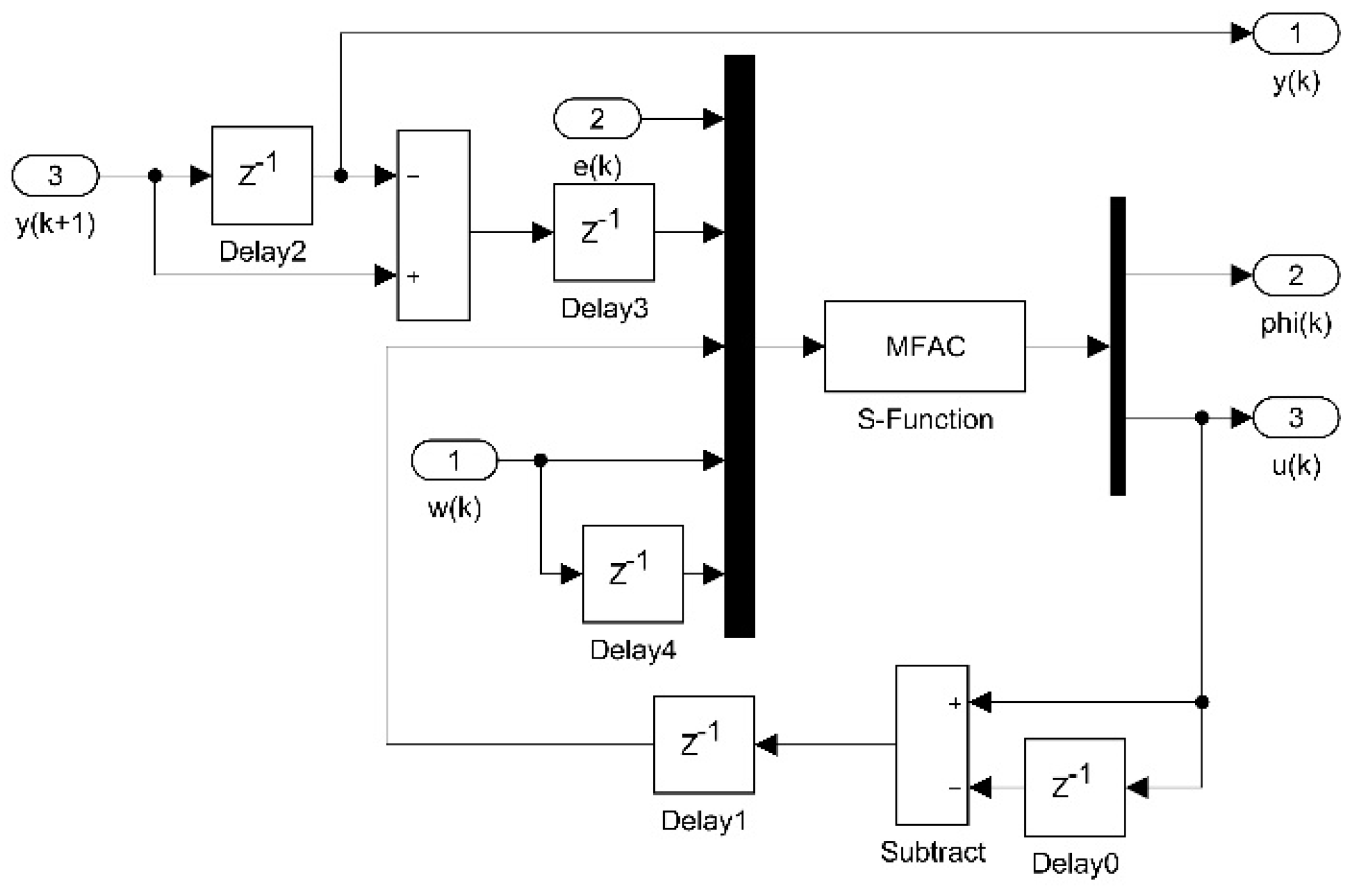
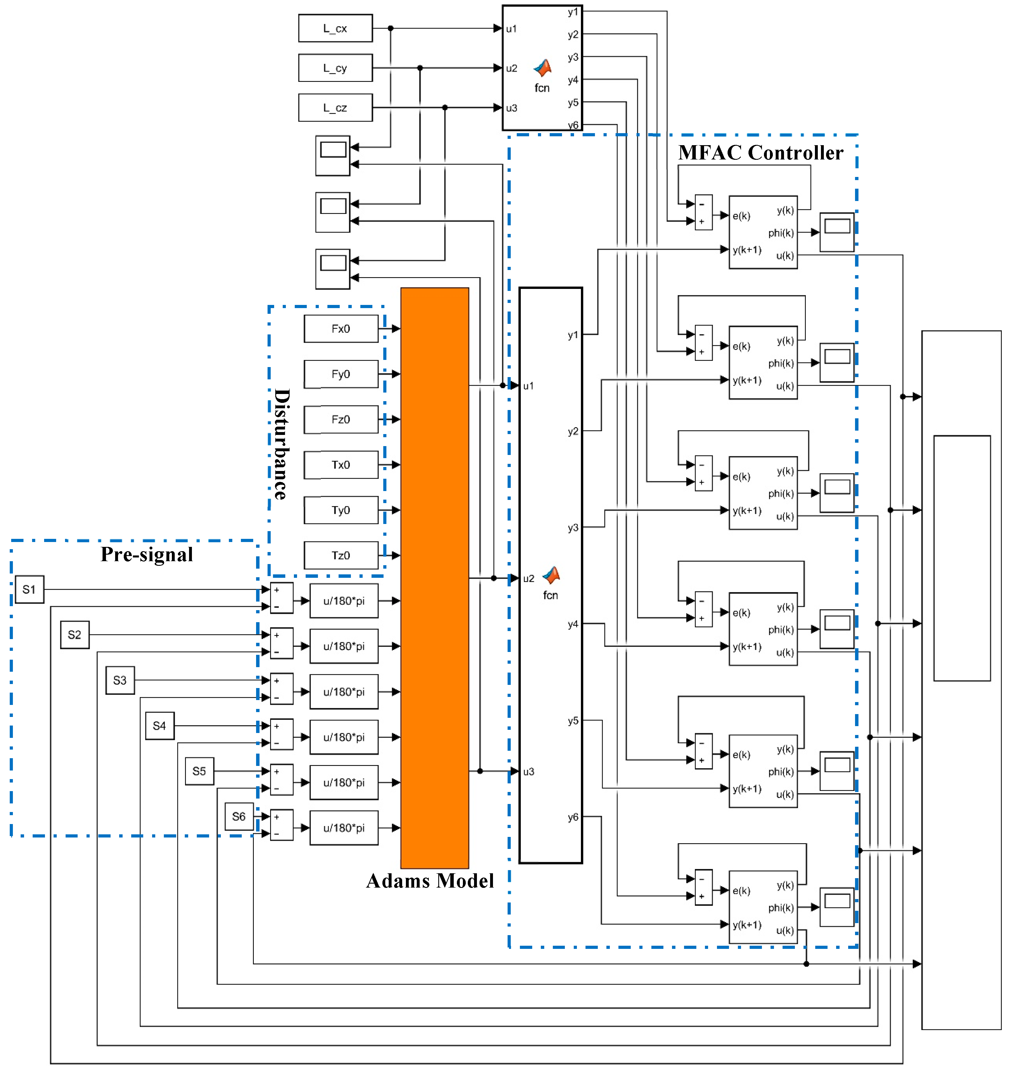
In summary, most control schemes for a UVMS are dependent on a complex mathematical model of UVMS. However, ocean current disturbance is random and the UVMS is a redundant system, so it is difficult to establish a precise kinematics model and dynamics model of UVMS, resulting in limited improvement of control accuracy. In addition, the universality of model-based control schemes is poor. Therefore, a model-free control scheme is necessary. 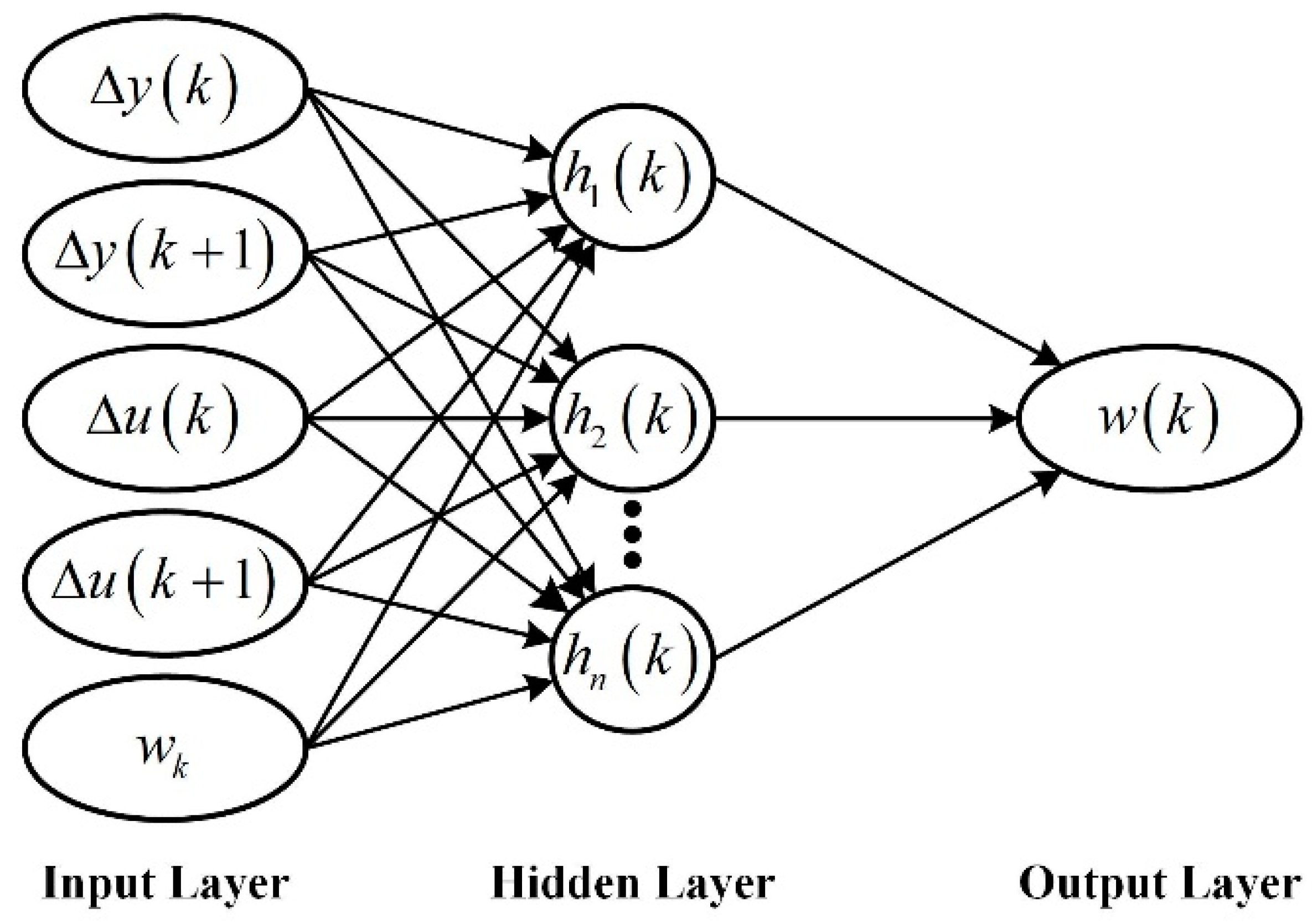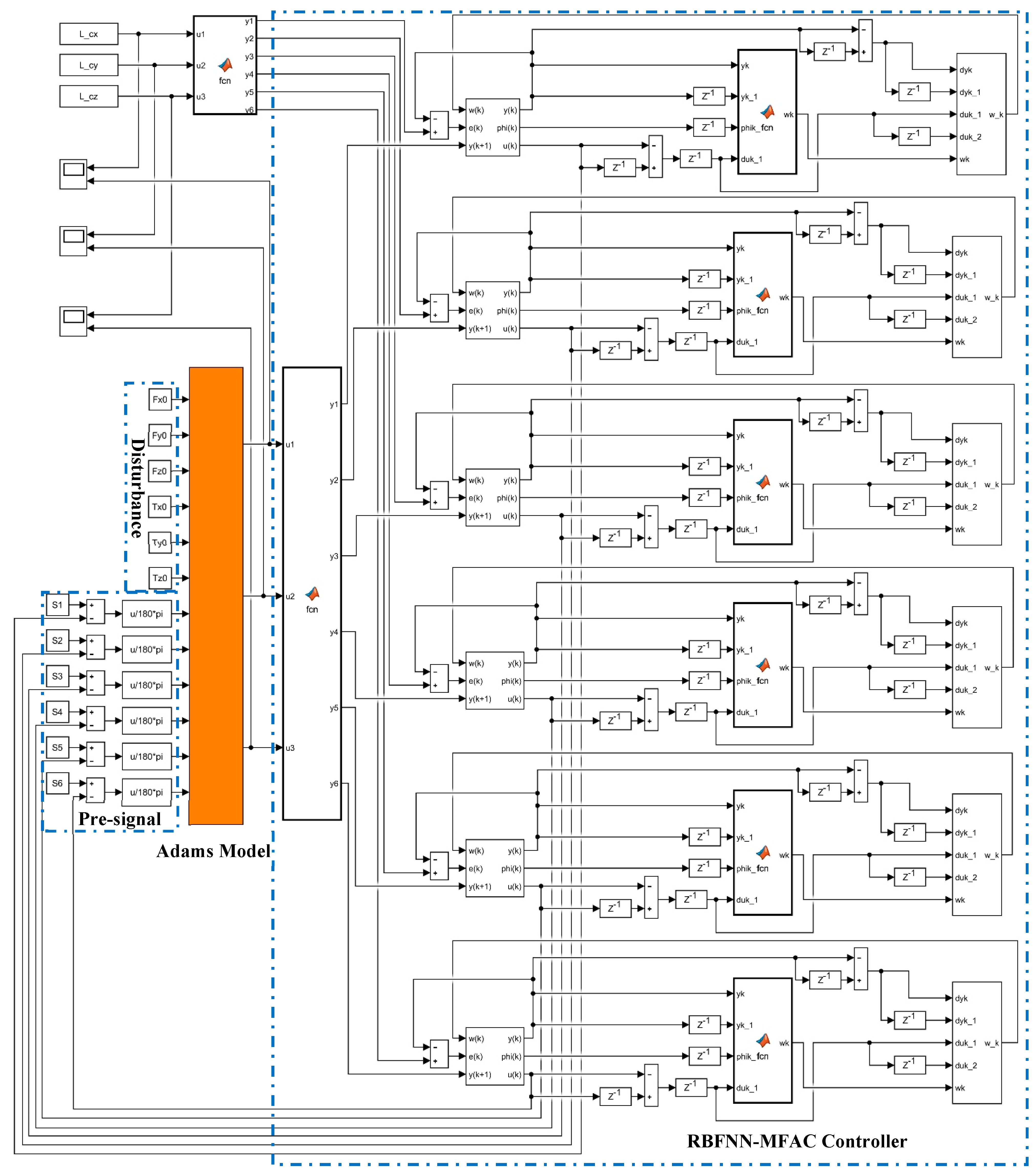Considering that the UVMS is a multivariable nonlinear time-varying system, a normal PID (Proportional Integral Derivative) controller cannot achieve high control accuracy, while the model-free adaptive control (MFAC) method has proven to be effective to deal with e multivariable nonlinear time-varying systems [25]. A UVMS is a complex nonlinear time-varying system, so estimation based on a time-varying bounded parameter in an MFAC is not accurate enough. Fortunately, the radial basis function neural network (RBFNN) is able to approximate nonlinear function accurately. Thus, the MFAC method combined with RBFNN, and the RBFNN-MFAC method should have better performance.

In our study, a UVMS consisting of a six degrees of freedom underwater vehicle and a six degrees of freedom manipulator was taken as the research object. The RBFNN-MFAC method was used to improve the trajectory tracking accuracy of a UVMS under uncertain disturbance conditions of ocean current. The paper is structured as follows. In Section 2, the hydrodynamic model of the UVMS is defined in commercial software (Fluent) and a mechanism dynamic model of the UVMS is defined in the commercial software, Adams. In Section 3, model-free control schemes, including PID, MFAC and RBFNN-MFAC, are designed. In Section 4, simulation results are visualized, the performance of each control scheme is discussed, and a physical prototype of the UVMS is developed. 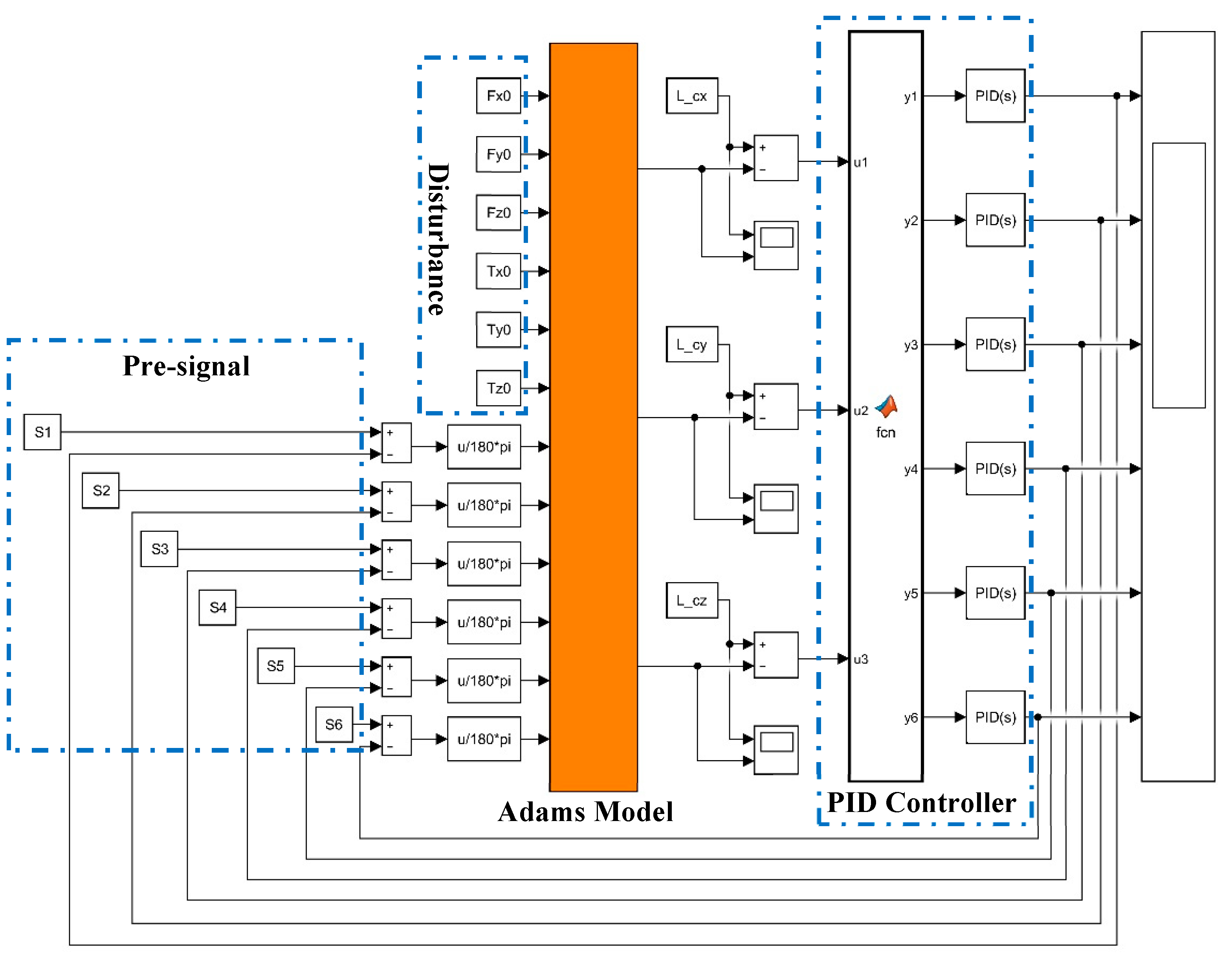In Section 5, the main conclusions of the paper are summarized, and suggestions for future research are made. To highlight the MFAC controller, a model-free control scheme was taken as a comparison, and a PID controller for the UVMS was designed. The numerical simulation model in this paper is only used to calculate the disturbance of the current and simulate the motion state of the UVMS. Considering the difficulties in establishment of the precise kinematics model and dynamics model of the UVMS, there is no need to use the result of numerical simulation model in the design of the RBFNN-MFAC controller. This demonstrates that the RBFNN-MFAC scheme does not depend on the kinematics model and dynamics model of the UVMS, and that the universality of the controller is good.

2. UVMS Model

2.1. Mechanical Structure of UVMS

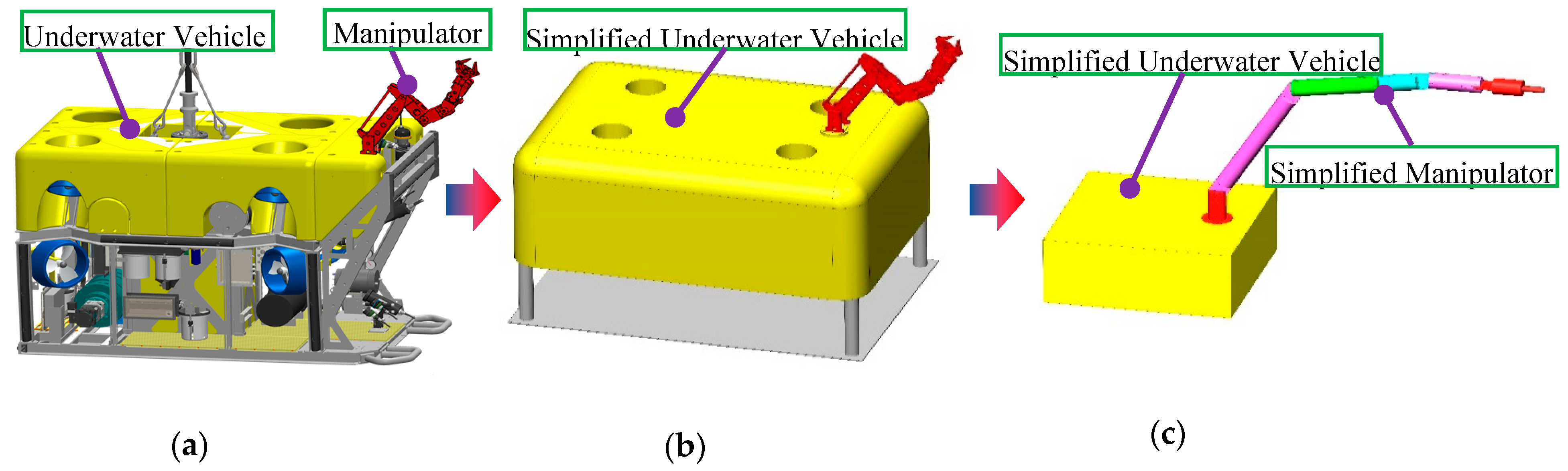
The underwater vehicle provides a basic platform for the underwater manipulator, and the installation position of manipulator is determined by the function of UVMS. The manipulator can be on the top [26], at the front [27] or on the bottom [28] of the underwater vehicle. Taking the manipulator installed on the top of the underwater vehicle as an example, a physical model of the UVMS is illustrated in Figure 1a. The underwater vehicle, with six degrees of freedom, is driven by four propellers in the horizontal direction and four propellers in the vertical direction. The manipulator, with six degrees of freedom, is mounted on the top of the underwater vehicle. The mass of the underwater vehicle is about 3939 kg, the mass of the manipulator is about 61 kg, and the total mass of the UVMS is about 4000 kg.

Figure 1. Mechanical Structure of UVMS. (a) Physical Model; (b) Model for Fluid Dynamics; (c) Model for Mechanism Dynamics.

The UVMS works in water, which means fluid dynamics analysis and the mechanism dynamics analysis are necessary. Fluent is a commercial Computational Fluid Dynamics (CFD) package for solving complex differential equations by a numerical approach [29], which was used to deal the fluid dynamics analysis in this work. Adams is professional multi-body dynamics simulation system software [30], which was used to deal with the mechanism dynamics analysis in this work. A simulation model based on Fluent and Adams software has been widely used in research on underwater robots [31] and cars [32]. The model’s accuracy has been validated in previous research.

A model of a UVMS for fluid dynamics analysis is illustrated in Figure 1b. A geometric model of the underwater vehicle was simplified, but the mass and the displacement volume of the underwater vehicle remained unchanged. The position and the structure of the manipulator remained unchanged. Compared with a physical model, the model for fluid dynamics did not change the hydrodynamics performance of the manipulator, and the shape of the underwater vehicle was kept unchanged as much as possible. Therefore, model simplification for fluid dynamics analysis was reasonable.

A model of a UVMS for mechanism dynamics analysis is illustrated in Figure 1c. The appearance of UVMS was further simplified, but the relative position, the relative motion and the constraint relationship between the underwater vehicle and the manipulator remained unchanged, and was the same for each joint of the manipulator. Relative position, relative motion and constraint relationship are key factors affecting mechanism dynamics performance. Compared with the physical model, those factors were unchanged in the model for mechanism dynamics. Therefore, the model simplification for mechanism dynamics analysis was reasonable. In the mechanism dynamics analysis process, the dimension of the underwater vehicle has no effect and the size of underwater vehicle is reasonably reduced, giving the impression that the manipulator is too long.

2.2. Fluid Dynamics Simulation Model

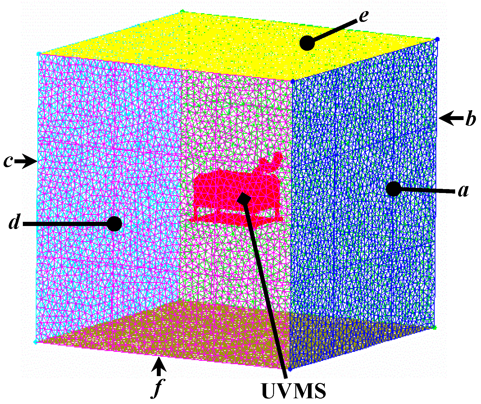
A three-dimensional flow field domain of the UVMS was established, as shown in Figure 2. The flow field was spatially discretized by mesh, and the boundaries were sequentially named to generate mesh files.

Figure 2. Flow Field Domain of the UVMS.

The dimensions of the UVMS were: length $L=2950$ mm, width $W=1800$ mm, height $H=2450$ mm. For the dimensions of the flow field domain, the length, the width and the height were the same, so that $L_f=W_f=H_f=10,000$ mm, and the boundary of the flow field was away from the UVMS. Each boundary panel, panel a, panel b, panel c, panel d, panel e and panel f could be used as the inlet boundary or outlet boundary of the flow field domain to simulate water flows in different directions. According to mesh independence verification, the minimum mesh size was set at 0.3 mm and the number of cells was 5,610,234.

Assuming that the water around UVMS is an incompressible fluid, the hydrodynamics of the flow field domain should follow the N-S equation, which describes the law of conservation of momentum for viscous incompressible fluids [33], as:

$$\frac{\partial \left(\rho u_i\right)}{\partial t}+\frac{\partial }{\partial x_i}\left(\rho u_i{u}_j\right)=-\frac{\partial p}{\partial x_i}+\frac{\partial }{\partial x_j}\left(\mu \frac{\partial u_i}{\partial x_j}-\rho \overline{u_i{}^{\prime }{u}_j{}^{\prime }}\right)+S_i$$

(1)

where $x_i$ is the coordinate value, $\rho$ is the fluid density, $t$ is the fluid motion time, $u_i$ is the time-average value of the velocity component, $u_i{}^{\prime }$ and $u_j{}^{\prime }$ are the fluctuating value of the velocity component, $\mu$ is the dynamic viscosity of fluid, and $S_i$ is the generalized source term.

In the simulation process, the mesh file was imported into Fluent software, the inlet boundary was set as the velocity inlet, the outlet boundary was set as the outflow, the other boundary of flow field was set as symmetry, and the surface boundary of UVMS was set as the wall. A standard $k-\epsilon$ turbulence model was selected to close the N-S equation.

In terms of the solver, a steady fluid dynamics analysis of the UVMS was conducted in this study, and a pressure-based solver was selected. The SIMPLE (Semi-Implicit Method for Pressure Linked Equations) scheme, which characterizes development in mass momentum coupled and pressure-based schemes [34], was used for the pressure-velocity coupling solution. In terms of spatial discretization, a least squares cell-based method was selected for the gradient term, a second order method was selected for the pressure term, a second-order upwind method was selected for the momentum term, and a first-order upwind method was used for the turbulent kinetic energy term and the turbulent dissipation rate term.

2.3. Mechanism Dynamics Simulation Model

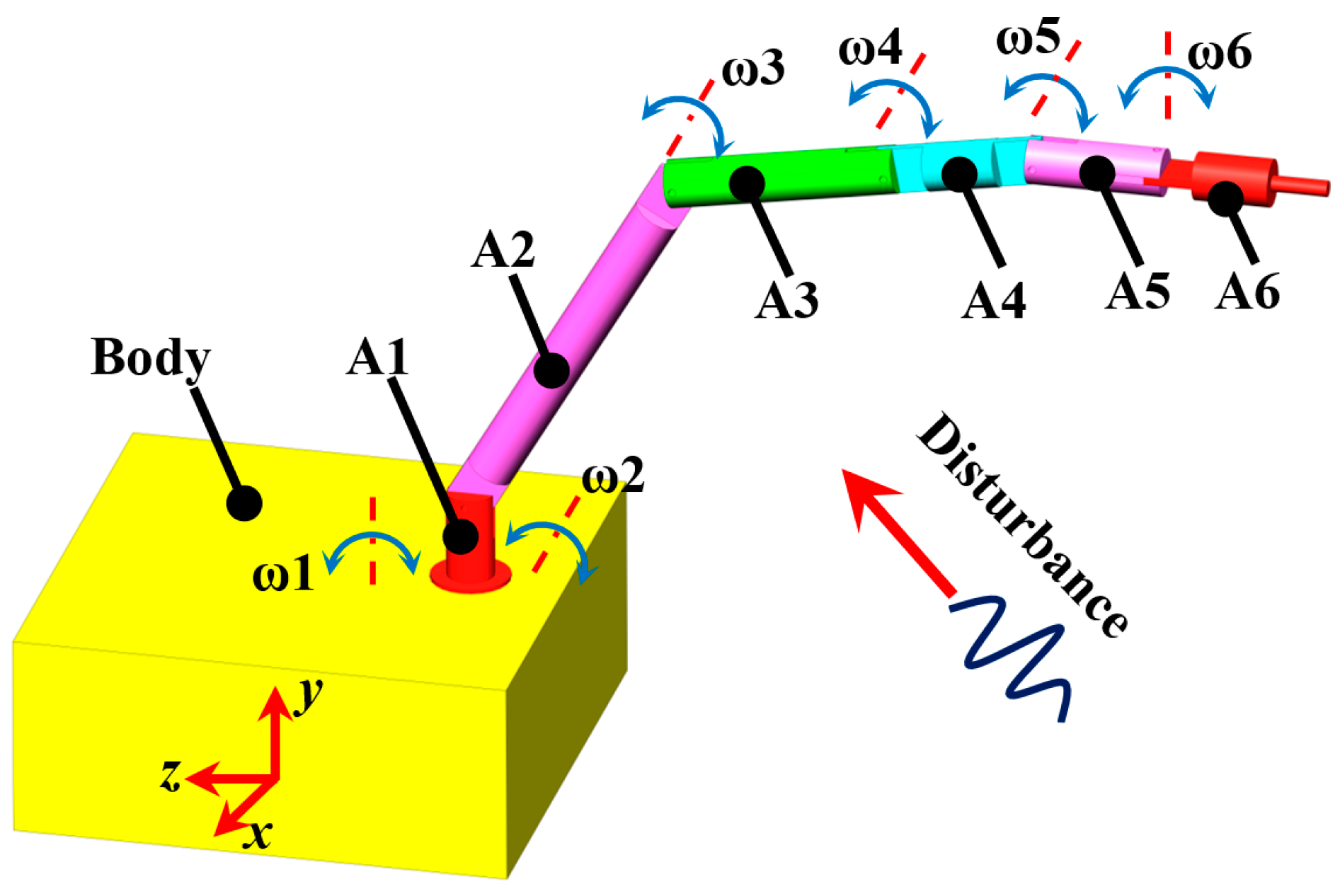
The motion of each UVMS joint and the load on UVMS is shown in Figure 3.

Figure 3. Motion of Joint and Load on UVMS.

The dimensions of each joint were $l_{A1}=100$ mm, $l_{A2}=525$ mm, $l_{A3}=270$ mm, $l_{A4}=190$ mm, $l_{A5}=150$ mm, and $l_{A6}=215$ mm. The operating radius of the underwater manipulator could be more than 1200 mm, and the manipulator had enough rigidity.

With the disturbance of ocean currents, the underwater vehicle is subjected to forces along the x-axis, the y-axis and the z-axis, as well as torque around the x-axis, the y-axis, and the z-axis. When the propellers are closed, the value of the force and the torque, which cause spatial motion of underwater vehicle, is related to the velocity of the ocean current. The fluid force on the manipulator is not only related to the velocity of ocean current, but also related to the motion speed of each joint, and the force direction changes with time. The fluid force, the motion speed and the control signal for each part of UVMS are listed in Table 1.

Table 1. Fluid Force, Motion Speed and Control Signal for Each Part of UVMS.

Part	Fluid Force	Motion Speed	Control Signal
Body	$F_x$$, F_y$$, F_z$ $T_x$$, T_y$$, T_z$	$v_x$$, v_y$$, v_z$ ${\omega }_x$$, {\omega }_y$$, {\omega }_z$	--
A1	$F_1$	${\omega }_1$	CS1
A2	$F_2$	${\omega }_2$	CS2
A3	$F_3$	${\omega }_3$	CS3
A4	$F_4$	${\omega }_4$	CS4
A5	$F_5$	${\omega }_5$	CS5
A6	$F_6$	${\omega }_6$	CS6

The mechanism dynamics equation of the multi-joint manipulator, which is commonly used in dynamic analysis [35], is as follows.

$${\mathit{M}}_m\left(\omega \right)\dot{\omega }+\mathit{C}\left(\omega \right)\omega +\mathit{G}\left(\omega \right)+\mathit{F}\left(\omega \right)+{\mathit{\tau }}_d=\mathit{\tau }$$

(2)

where ${\mathit{M}}_m\left(\omega \right)$ is the n order inertial matrix, $\mathit{C}\left(\omega \right)$ is the n order resultant force matrix of the centripetal force and the Coriolis force, $\mathit{G}\left(\omega \right)$ is the equivalent gravity, $\mathit{F}\left(\omega \right)$ is the friction force matrix, ${\mathit{\tau }}_d$ is the disturbance force, and $\mathit{\tau }$ is the driven force.

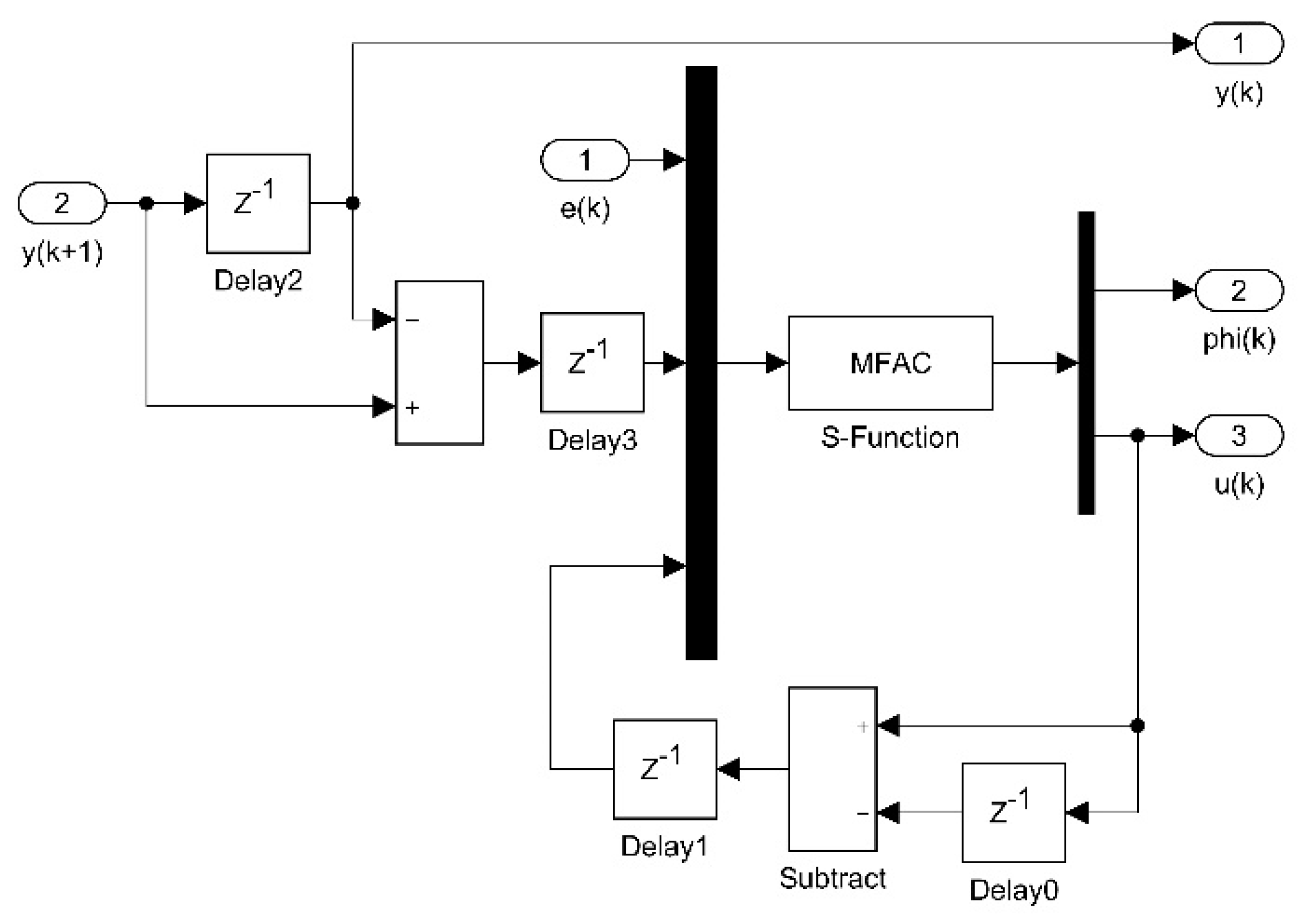
In the simulation process, the model for mechanism dynamics was imported into Adams software, and the mass, the centroid position, and the rotation inertia of each part were defined according to the physical model. The constraint relationship among each part was added as well. The Adams numerical simulation model was exported to the Simulink module, and the Adams-Simulink joint simulation model was generated.

3. Control Scheme

3.1. PID Control Scheme

Most control schemes, such as the sliding mode control approach, are model based control schemes. In this study, considering the difficulties concerning establishment of a precise kinematics model and a dynamics model of the UVMS, a model-free control scheme was proposed. Fortunately, the PID control scheme, which has been widely used in a variety of applications [36], is a typical model-free control scheme. Therefore, the PID control scheme was taken as a comparative scheme for trajectory tracking control of the UVMS. The PID based Simulink controller model is shown in Figure 4.

Figure 4. PID Based Simulink Controller Model.

The Adams model of the UVMS was set as the controlled object. The fluid forces on the underwater vehicle were imported into Adams as $F{x}_0$, $F{y}_0$, $F{z}_0$, $T{x}_0$, $T{y}_0$, $F{z}_0$. The fluid force on the manipulator can be calculated based on the hydrodynamic coefficient set in Adams automatically. L_cx, L_cy and L_cz were the desired motion trajectories of the manipulator endpoint. S1, S2, S3, S4, S5 and S6 were the pre-set control signals for motion trajectory tracking of each manipulator joint when that the fluid force was not considered.

In order to distribute the motion trajectory tracking error to the six controllers, an error distribution function was established.

$$\left[\begin{array}{l}y1\\ y2\\ y3\\ y4\\ y5\\ y5\end{array}\right]=\left[\begin{array}{ccc}{\xi }_{11}& {\xi }_{12}& {\xi }_{13}\\ {\xi }_{21}& {\xi }_{22}& {\xi }_{23}\\ {\xi }_{31}& {\xi }_{32}& {\xi }_{33}\\ {\xi }_{41}& {\xi }_{42}& {\xi }_{43}\\ {\xi }_{51}& {\xi }_{52}& {\xi }_{53}\\ {\xi }_{61}& {\xi }_{62}& {\xi }_{63}\end{array}\right]\left[\begin{array}{l}u1\\ u2\\ u3\end{array}\right]$$

(3)

where $u$ is the difference between the actual motion trajectory and the desired trajectory of manipulator endpoint, $\xi$ is the error distribution coefficient, and $y$ is the input signal of each joint controller. The definition of $\xi$ is related to the geometric characteristic parameters and the limited motion position of each joint.

The transfer function of PID control scheme is as follows.

$$F\left(s\right)=P+I\frac{1}{s}+D\frac{Ns}{s+N}$$

(4)

where $P$ is the proportional gain, $I$ is the integral gain, $D$ is the derivative gain, and $N$ is the filter coefficient.

3.2. MFAC Control Scheme

MFAC is a data-driven control method that does not rely on a kinematics model and a dynamics model. Hou et al. [37] addressed the bounded-input bounded-output stability, the monotonic convergence of the tracking error dynamics, and the internal stability of the full-form dynamic linearization of the MFAC control scheme, which will not be repeated in this paper.

The MFAC control scheme was designed as follows.

$$\widehat{\varphi }\left(k\right)=\widehat{\varphi }\left(k-1\right)+\frac{\eta \mathsf{\Delta }u\left(k-1\right)}{\mu +\mathsf{\Delta }u{\left(k-1\right)}^2}\left(\mathsf{\Delta }y\left(k\right)-\widehat{\varphi }\left(k-1\right)\mathsf{\Delta }u\left(k-1\right)\right)$$

(5)

• when $\mathsf{\Delta }u\left(k\right)\ne 0$, $\mathsf{\Delta }y\left(k+1\right)=\varphi \left(k\right)\mathsf{\Delta }u\left(k\right)$.
• when $\left|\widehat{\varphi }\left(k\right)\right|\le \epsilon$ or $\left|\mathsf{\Delta }u\left(k-1\right)\right|\le \epsilon$, $\widehat{\varphi }\left(k\right)=\widehat{\varphi }\left(1\right)$.
• where $y\left(k\right)$ is the actual motion trajectory of the manipulator, $u\left(k\right)$ is the control signal, $\varphi \left(k\right)$ is a time-varying bounded parameter, $\eta$ is the step sequence, and $\mu$ is the weight factor.

The control signal is defined as follows.

$$u\left(k\right)=u\left(k-1\right)+\frac{\kappa \widehat{\varphi }\left(k\right)}{\lambda +{\left|\widehat{\varphi }\left(k\right)\right|}^2}\left(y^{*}\left(k+1\right)-y\left(k\right)\right)$$

(6)

where $\kappa$ is the step sequence, $\lambda$ is the weight factor.

Based on above equations, the workflow of MFAC can be generalized, as illustrated in Figure 5.

Figure 5. Workflow Chart of MFAC.

The parameters that need to be tuned in the MFAC controller are $\eta$, $\mu$, $\kappa$ and $\lambda$.

The MFAC based Simulink controller model is shown in Figure 6.

Figure 6. MFAC Based Simulink Controller Model.

The kernel of the MFAC controller is shown in Figure 7.

Figure 7. Kernel of MFAC Controller.

3.3. RBFNN-MFAC Control Scheme

To further improve the motion trajectory tracking accuracy, a radial basis function neural network was embedded into the MFAC control scheme. The RBFNN control scheme was used to predict the value of the pseudo-partial derivative $\varphi \left(k\right)$. The topology structure of the RBFNN is shown in Figure 8.

Figure 8. Topology Structure of RBFNN.

A neural network consists of one input layer, one hidden layer and one output layer. Historical information is included in the input system. The output value of RBFNN is as follows.

$$w_k=y\left(k+1\right)-y\left(k\right)+\varphi \left(k\right)\left(u\left(k+1\right)-u\left(k\right)\right)$$

(7)

The RBFNN-MFAC-based Simulink controller model is shown in Figure 9.

Figure 9. RBFNN-MFAC based on a Simulink Controller Model.

The kernel of the RBFNN-MFAC controller is shown in Figure 10.

Figure 10. Kernel of the RBFNN-MFAC Controller.

Therefore, Equation (5) can be rewritten as follows.

$$\widehat{\varphi }\left(k\right)=\widehat{\varphi }\left(k-1\right)+\frac{\eta \mathsf{\Delta }u\left(k-1\right)}{\mu +\mathsf{\Delta }u{\left(k-1\right)}^2}\left(\mathsf{\Delta }y\left(k\right)-\widehat{\varphi }\left(k-1\right)\mathsf{\Delta }u\left(k-1\right)\right)-\frac{\eta \mathsf{\Delta }u\left(k-1\right)w\left(k+1\right)}{\mu +\mathsf{\Delta }u{\left(k-1\right)}^2}$$

(8)

Equation (6) can be rewritten as follows.

$$u\left(k\right)=u\left(k-1\right)+\frac{{\rho }_1\widehat{\varphi }\left(k\right)\left(y^{*}\left(k+1\right)-y\left(k\right)\right)}{\lambda +{\left|\widehat{\varphi }\left(k\right)\right|}^2}-\frac{{\rho }_2\widehat{\varphi }\left(k\right)w\left(k\right)}{\lambda +{\left|\widehat{\varphi }\left(k\right)\right|}^2}$$

(9)

4. Results and Discussion

4.1. Simulation Initialization

The ocean current generally occurs in a horizontal direction. Thus, disturbance along the ±y axis direction was ignored. The ocean current flow velocities along the +z axis direction, the +x axis direction, the −z axis direction and the −x axis were individually set as $v_{\max }=0.2 \mathrm{m}/\mathrm{s}$. The steady hydrodynamic force of each UVMS joint was calculated, as shown in Table 2.

Table 2. Steady Hydrodynamic Force of Each UVMS Joint.

Part	${\mathit{F}}_{+\mathit{z}}$	${\mathit{F}}_{+\mathit{x}}$	${\mathit{F}}_{-\mathit{z}}$	${\mathit{F}}_{-\mathit{x}}$
Body	606.5 N	545.0 N	502.4 N	576.9 N
A1	0.1 N	14.0 N	6.7 N	−0.5 N
A2	25.8 N	9.0 N	−11.0 N	4.6 N
A3	18.1 N	5.1 N	−9.5 N	3.7 N
A4	14.2 N	2.7 N	−9.4 N	1.3 N
A5	5.3 N	1.4 N	−1.8 N	2.1 N
A6	9.3 N	8.5 N	2.3 N	2.6 N

A negative value indicates that the hydrodynamic force direction was opposite to the ocean current direction.

Considering that the shape of UVMS is complex, various ocean current directions cause various hydrodynamic force. It is difficult to calculate the hydrodynamic force in every ocean current direction. Therefore, a disturbance function was designed to simplify the disturbance effect caused by ocean current as follows.

$${\tau }_n=\frac{v_n^2}{v_{\max }^2}\left(\begin{array}{cccc}{\gamma }_{+zn}& {\gamma }_{+zn}& {\gamma }_{-zn}& {\gamma }_{-xn}\end{array}\right)\left(\begin{array}{c}{F}_{+zn}\\ F_{+xn}\\ F_{-zn}\\ F_{-xn}\end{array}\right)$$

(10)

where $v_n$ is the motion speed of each UVMS joint, and $\gamma$ is the random number in the range of (−1, 1).

Disturbance was added to the Adams mechanism dynamics model of the UVMS through the Simulink module.

The parameters for PID control scheme are listed in Table 3.

Table 3. Parameters for PID Control Scheme.

Part	P	I	D
A1	0.0031	0.021	0.0013
A2	0.0029	0.022	0.0015
A3	0.0072	0.031	0.0014
A4	0.0082	0.054	0.0021
A5	0.0027	0.033	0.0009
A6	0.0031	0.026	0.0017

The parameters for MFAC control scheme are listed in Table 4.

Table 4. Parameters for MFAC Control Scheme.

Part	$\mathit{\eta }$	$\mathit{\mu }$	$\mathit{\rho }$	$\mathit{\lambda }$
A1	0.11	0.74	0.21	31
A2	0.11	0.74	0.11	15
A3	0.11	0.74	0.9	7
A4	0.11	0.74	0.17	6
A5	0.11	0.74	0.03	13
A6	0.11	0.74	0.09	19

The parameters for the RBFNN-MFAC control scheme are similar to that for the control scheme. The momentum factor of the RBF neural network was set as $\alpha =0.9$, and the learning rate of RBF neural network was set as $\beta =0.6$.

The error distribution coefficient matrix was set as follows.

$$\left[\begin{array}{ccc}{\xi }_{11}& {\xi }_{12}& {\xi }_{13}\\ {\xi }_{21}& {\xi }_{22}& {\xi }_{23}\\ {\xi }_{31}& {\xi }_{32}& {\xi }_{33}\\ {\xi }_{41}& {\xi }_{42}& {\xi }_{43}\\ {\xi }_{51}& {\xi }_{52}& {\xi }_{53}\\ {\xi }_{61}& {\xi }_{62}& {\xi }_{63}\end{array}\right]=\left[\begin{array}{ccc}0.32& 0& 0.07\\ 0& 0.46& 0.36\\ 0& 0.24& 0.19\\ 0& 0.17& 0.13\\ 0& 0.13& 0.1\\ 0.68& 0& 0.15\end{array}\right]$$

4.2. Position Tracking Error

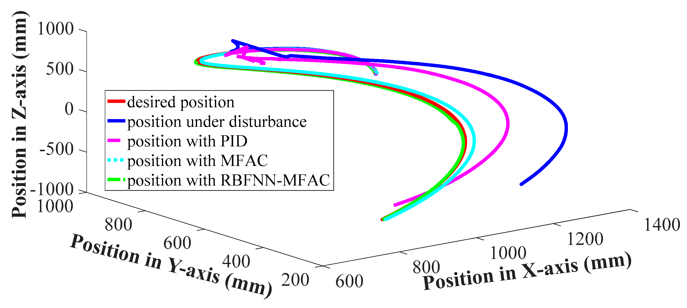
Motion trajectory of manipulator endpoints with various control schemes are shown in Figure 11.

Figure 11. Motion Trajectory of Manipulator Endpoint with Various Control Schemes.

As shown in Figure 11, with the effect of ocean current disturbance, the actual motion trajectory of manipulator endpoint significantly deviated from the desired motion trajectory without the feedback control method, i.e., the curve designated as position under disturbance. When the PID control scheme was added, the tracking error was slightly reduced, but the position tracking accuracy at the final moment was greatly improved. When the MFAC control scheme and the RBFNN-MFAC control scheme were used, the position tracking accuracy was significantly improved.

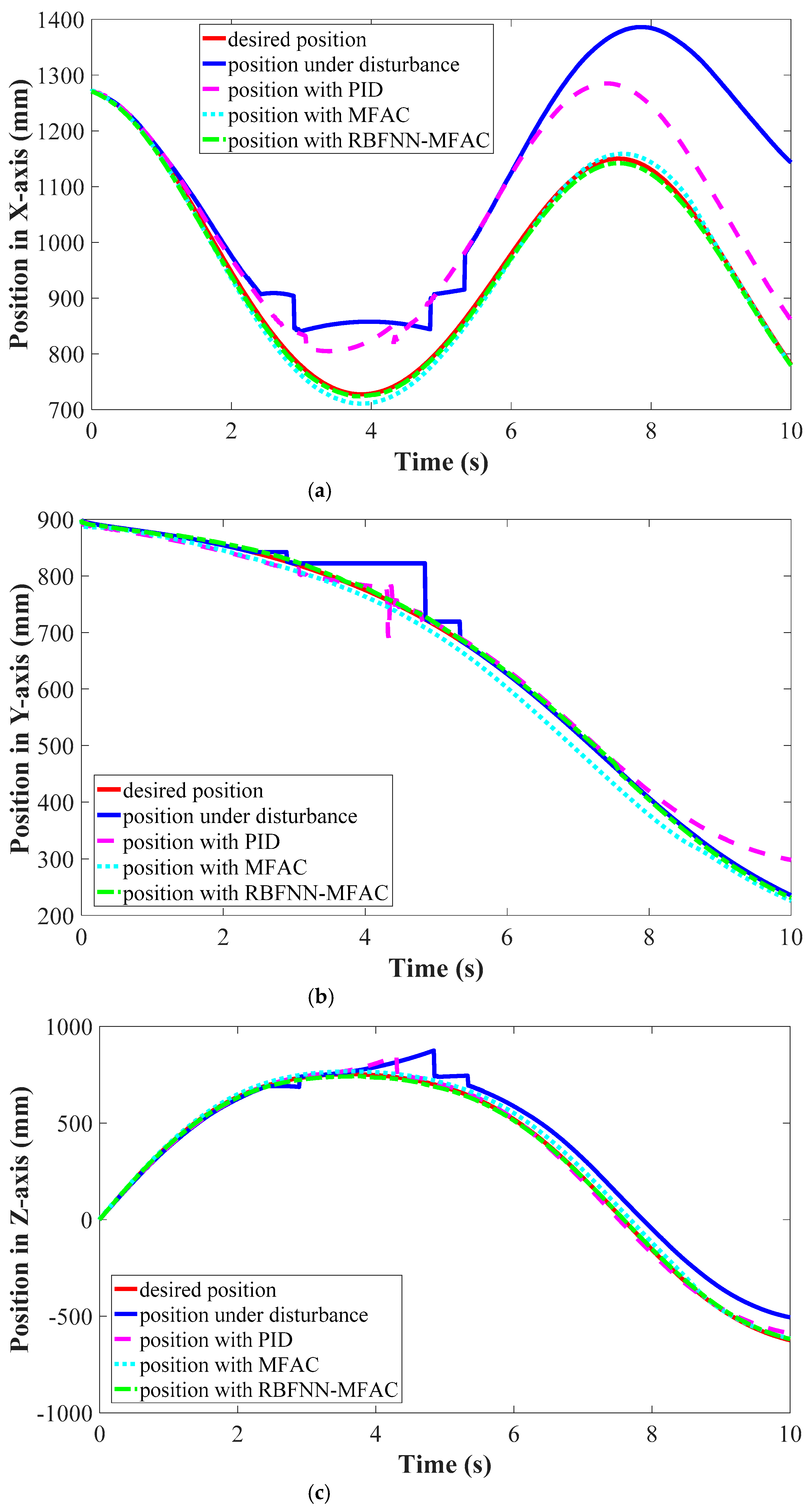
The position tracking accuracy along x axis, y axis and z axis of Cartesian coordinates is shown in Figure 12.

Figure 12. Position Tracking Accuracy along Various Axes of Cartesian Coordinates. (a) Position Tracking Accuracy along the x Axis; (b) Position Tracking Accuracy along the y Axis; (c) Position Tracking Accuracy along the z Axis.

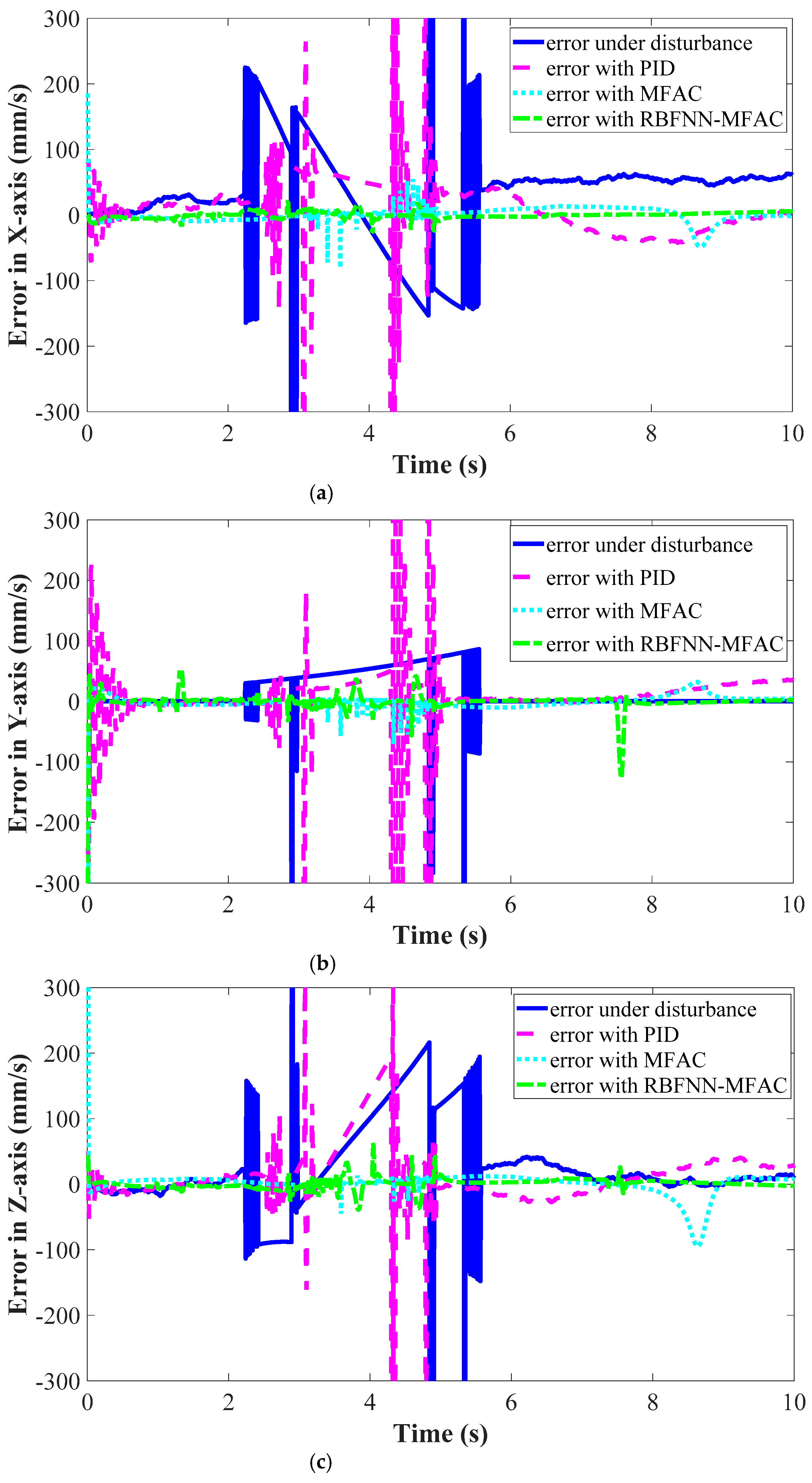
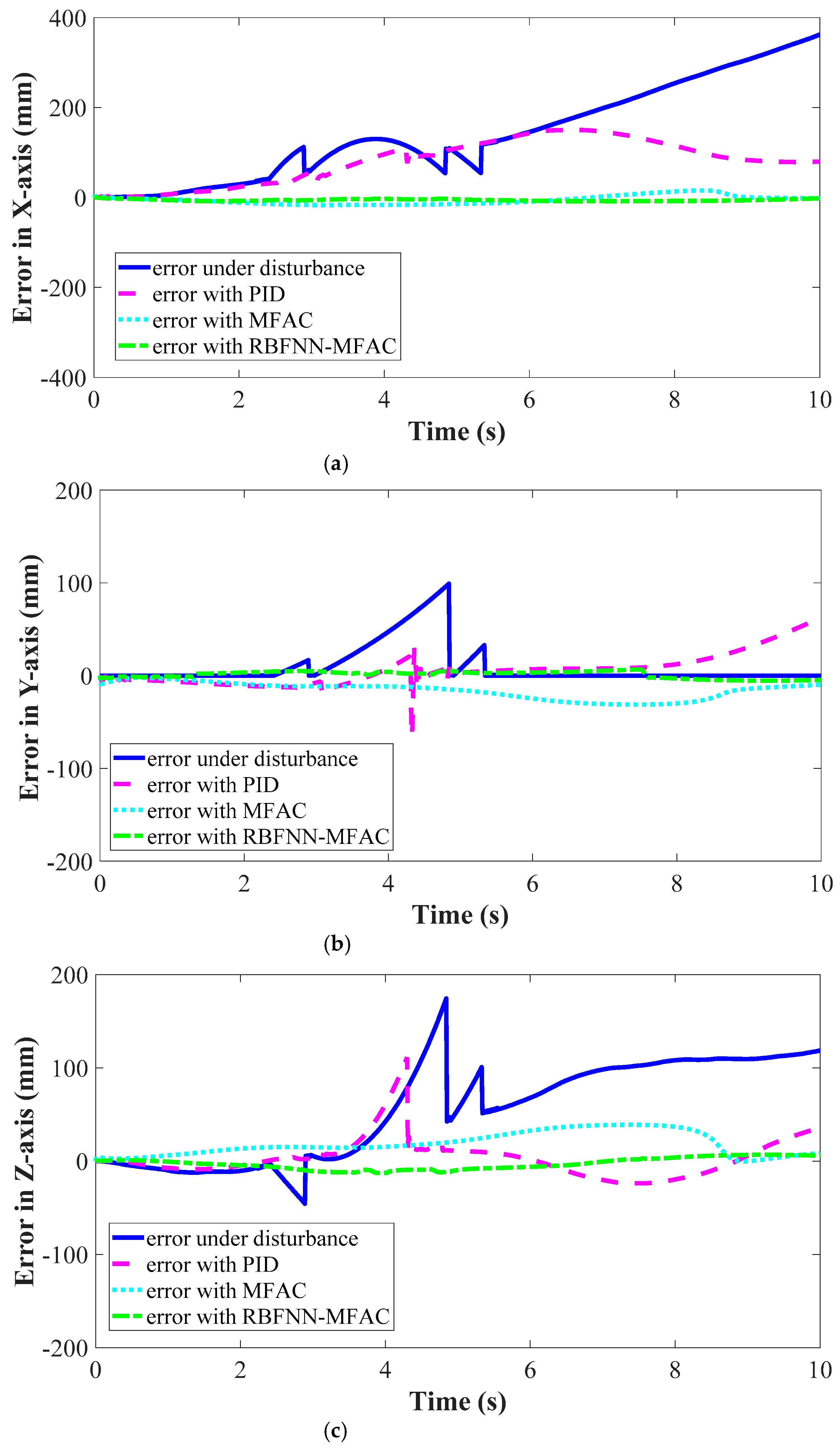
Furthermore, $e_p$ was defined as the difference between the simulated position and the desired position. The position tracking error, $e_p$, was calculated, as shown in Figure 13.

Figure 13. Position Tracking Error along Various Axes of Cartesian Coordinates. (a) Position Tracking Error along x Axis; ($e_{px}$: average error with PID is 80.1 mm, average error with MFAC is 9.3 mm, average error with RBFNN-MFAC is 5.8 mm). (b) Position Tracking Error along y Axis; ($e_{py}$: average error when PID is 12.9 mm, average error with MFAC is 15.9 mm, average error with RBFNN-MFAC is 3.5 mm). (c) Position Tracking Error along z Axis; ($e_{pz}$: average error when PID is 14.2 mm, average error with MFAC is 18.7 mm, average error with RBFNN-MFAC is 5.7 mm).

It can be seen that the position tracking error along x axis was the largest, which indicates that ocean current had the greatest influence on motion in x axis direction. The disturbance rejection function of MFAC and RBFNN-MFAC was most effective along the x axis to significantly improve the position tracking accuracy. The disturbance rejection function along y axis and z axis of RBFNN-MFAC was more effective than that of the MFAC.

The total average error with various control scheme was calculated as follows.

$$e=\sqrt{e_x^2+e_y^2+e_z^2}$$

(11)

Therefore, in terms of position tracking accuracy, $e_p$ with PID was 82.4 mm, $e_p$ with MFAC was 26.2 mm, and $e_p$ with RBFNN-MFAC was 8.9 mm. The position tracking accuracy of MFAC was 68.1% better than that of PID, and the position tracking accuracy of RBFNN-MFAC was 66.3% better than that of MFAC.

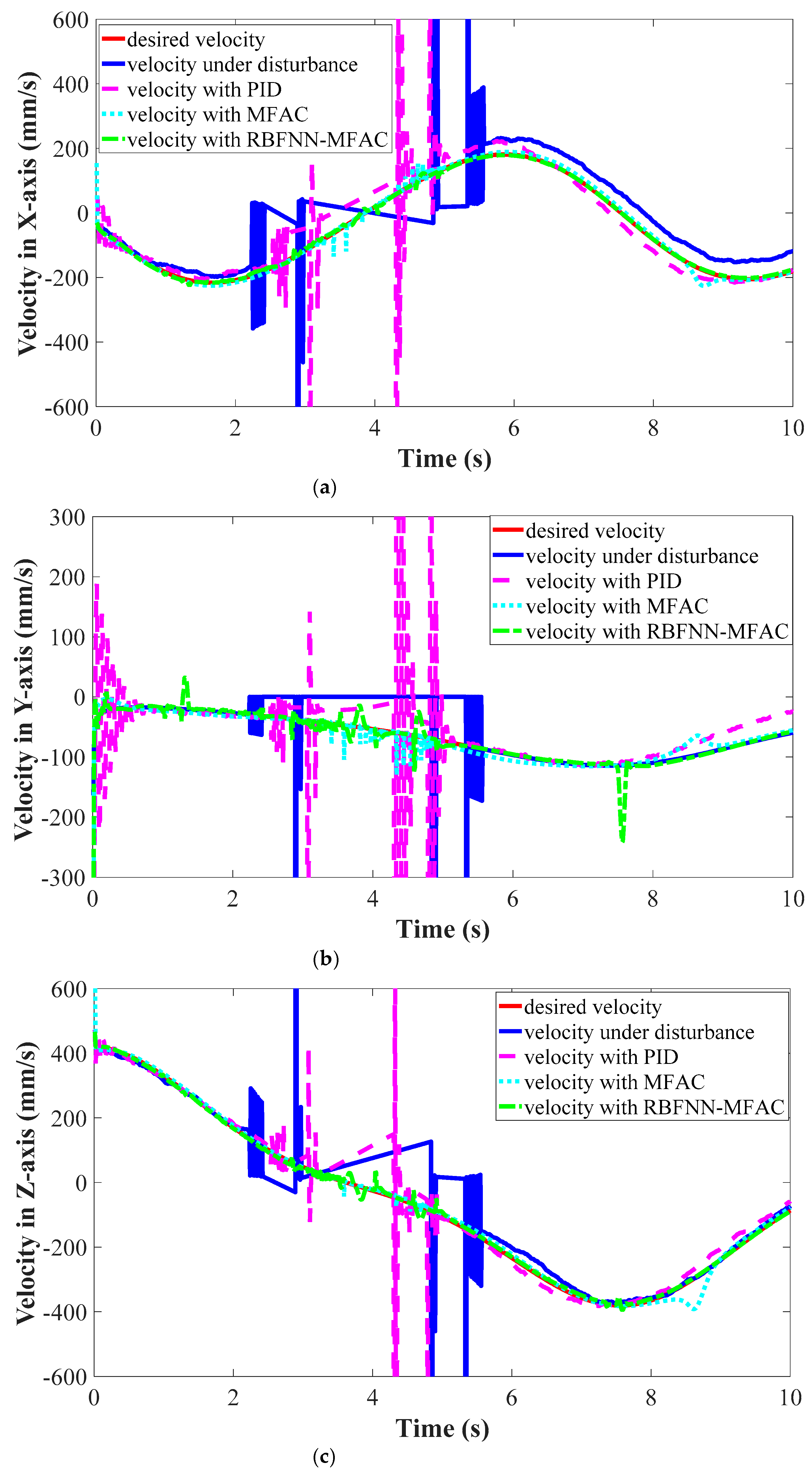
4.3. Speed Tracking Error

Although speed tracking accuracy was not the direct control objective, the control scheme works on the speed tracking accuracy. The speed tracking accuracy along x axis, y axis and z axis of Cartesian coordinates is shown in Figure 14.

Figure 14. Speed Tracking Accuracy along Various Axes of Cartesian Coordinates. (a) Speed Tracking Accuracy along x Axis. (b) Speed Tracking Accuracy along y Axis. (c) Speed Tracking Accuracy along z Axis.

Furthermore, $e_v$ was defined as the difference between the simulated velocity and the desired velocity. The speed tracking error, $e_v$, was calculated, as shown in Figure 15.

Figure 15. Speed Tracking Error along Various Axes of Cartesian Coordinates. (a) Speed Tracking Error along x Axis; ($e_{vx}$: average error with PID is 39.4 mm/s, average error with MFAC is 8.0 mm/s, average error with RBFNN-MFAC is 3.4 mm/s). (b) Speed Tracking Error along y Axis; ($e_{vy}$: average error when PID is 49.4 mm/s, average error with MFAC is 7.2 mm/s, average error with RBFNN-MFAC is 5.2 mm/s). (c) Speed Tracking Error along z Axis; ($e_{vz}$: average error with PID is 41.3 mm/s, average error when MFAC is 9.5 mm/s, and the average error with RBFNN-MFAC is 5.3 mm/s).

It can be seen that the MFAC and the RBFNN-MFAC caused the motion of the manipulator endpoint to be smoother, which meant the two control schemes had better disturbance rejection functions. Compared with MFAC, RBFNN-MFAC had better trajectory tracking performance.

In terms of speed tracking accuracy, $e_v$ with PID was 75.5 mm/s, $e_v$ with MFAC was 14.4 mm/s, and $e_v$ with RBFNN-MFAC was 8.2 mm/s. The speed tracking accuracy of MFAC was 81.0% better than that of PID, and the speed tracking accuracy of RBFNN-MFAC was 43.1% better than that of MFAC.

4.4. Physical Prototype and Future Work

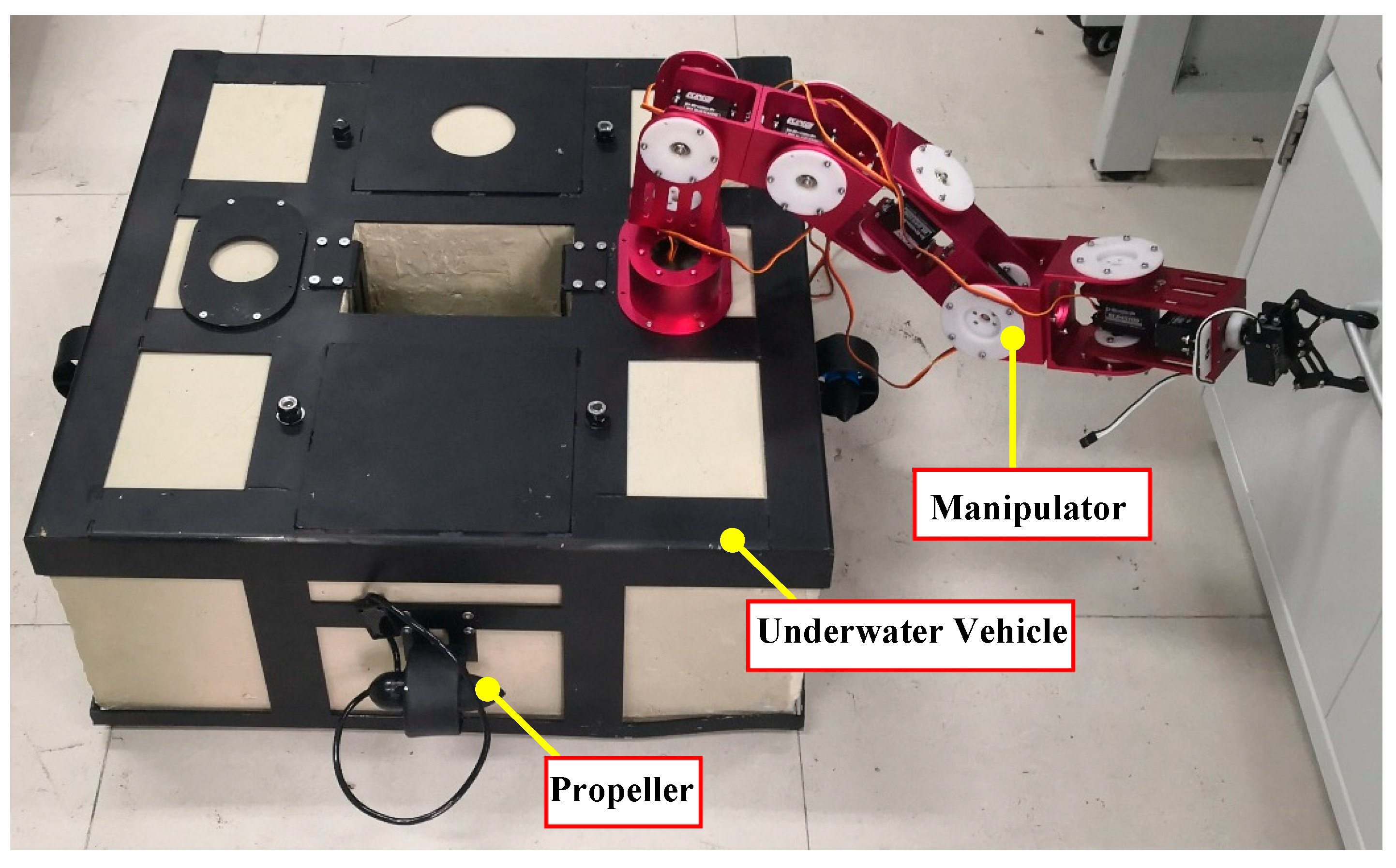
To verify the trajectory tracking performance of the proposed MFAC scheme and RBFNN-MFAC scheme in the future, a UVMS physical prototype was designed and manufactured, as shown in Figure 16.

Figure 16. UVMS Physical Prototype.

The underwater vehicle subsystem has a length of 600 mm, a width of 600 mm and a height of 250 mm. The total length of the manipulator subsystem is about 500 mm. The underwater vehicle has four propellers in the horizontal direction and two propellers in the vertical direction. The manipulator is driven by waterproof motors to ensure that the UVMS can work underwater.

Because of the lack of ocean current disturbance condition, the physical prototype has not been adequately tested in experiment. More sensors and batteries are needed to install on the physical prototype as well. Therefore, there is still much work to be done before the UVMS can work properly.

5. Conclusions

In this study, a UVMS consisting of a six degrees of freedom underwater vehicle and a six degrees of freedom manipulator was taken as the research object. The mechanical structure of UVMS was introduced. The ocean current disturbance on UVMS was analyzed by the commercial Fluent software, and the mechanism dynamics of UVMS was analyzed by Adams commercial software. The trajectory tracking performances of PID, MFAC and RBFNN-MFAC were analyzed by the Adams and Simulink joint simulation.

The results show that the position tracking accuracy with MFAC was 68.1% better than that with PID, the position tracking accuracy with RBFNN-MFAC was 66.3% better than that with MFAC, the speed tracking accuracy with MFAC was 81.0% better than that with PID, and the speed tracking accuracy with RBFNN-MFAC was 43.1% better than that with MFAC.

The proposed MFAC scheme and RBFNN-MFAC scheme does not depend on a kinematics model and dynamics model of the UVMS. Therefore, the universality of the controller is good, and the method is of great importance to applications in engineering.

In the future, experiments with various control schemes will be conducted based on the UVMS physical prototype to verify the trajectory tracking performance of the proposed MFAC scheme and RBFNN-MFAC scheme.