
Mesoscale Dynamics and Eddy Heat Transport in the Japan/East Sea from 1990 to 2010: A Model-Based Analysis


Abstract
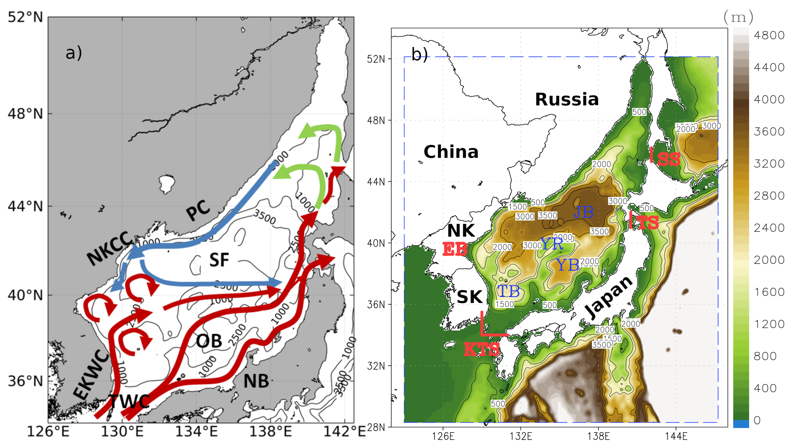
1. Introduction
2. Model Configuration and Setup of the Simulations
3. Model Validation
- Monthly mean satellite altimetry from the AVISO dataset (https://www.aviso.altimetry.fr/en/data/data-access.html, accessed on 1 December 2021) with a spatial resolution of 0.25 in longitude and latitude covering the time period from 1994 to 2010;
- Monthly mean sea surface height from the GOFS3.1 reanalysis [53] with a spatial resolution of 1/12 in longitude and latitude covering the time period from 1994 to 2010;
- Monthly climatological temperature from the East Asian Seas Regional Climatology (EAS dataset) [54] with a spatial resolution of 1/10 in longitude and latitude covering the time period from 1804 to 2013;
- Monthly mean transport estimations through the Korea/Tsushima Strait based on in situ observations from 1997 to 2007 [55];
3.1. Simulated Long-Term Mean Geostrophic Circulation in the Japan/East Sea
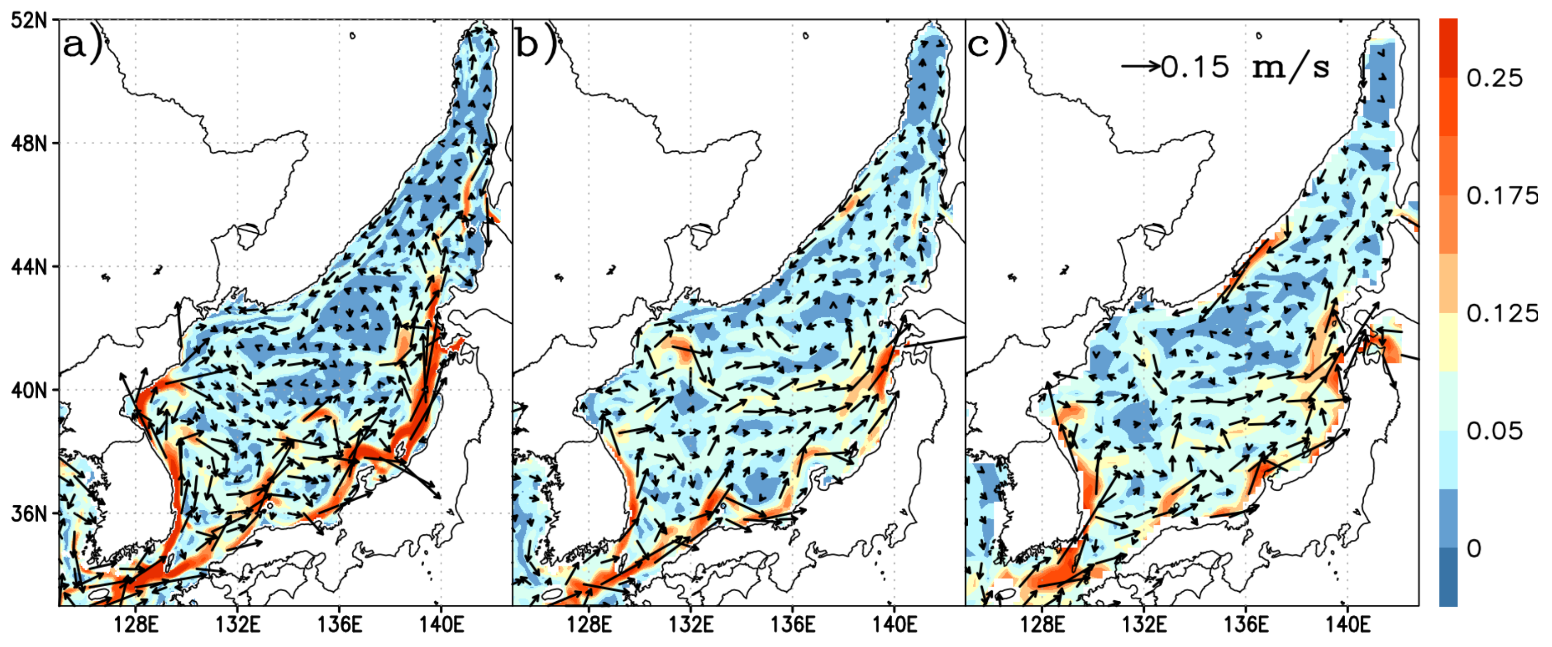
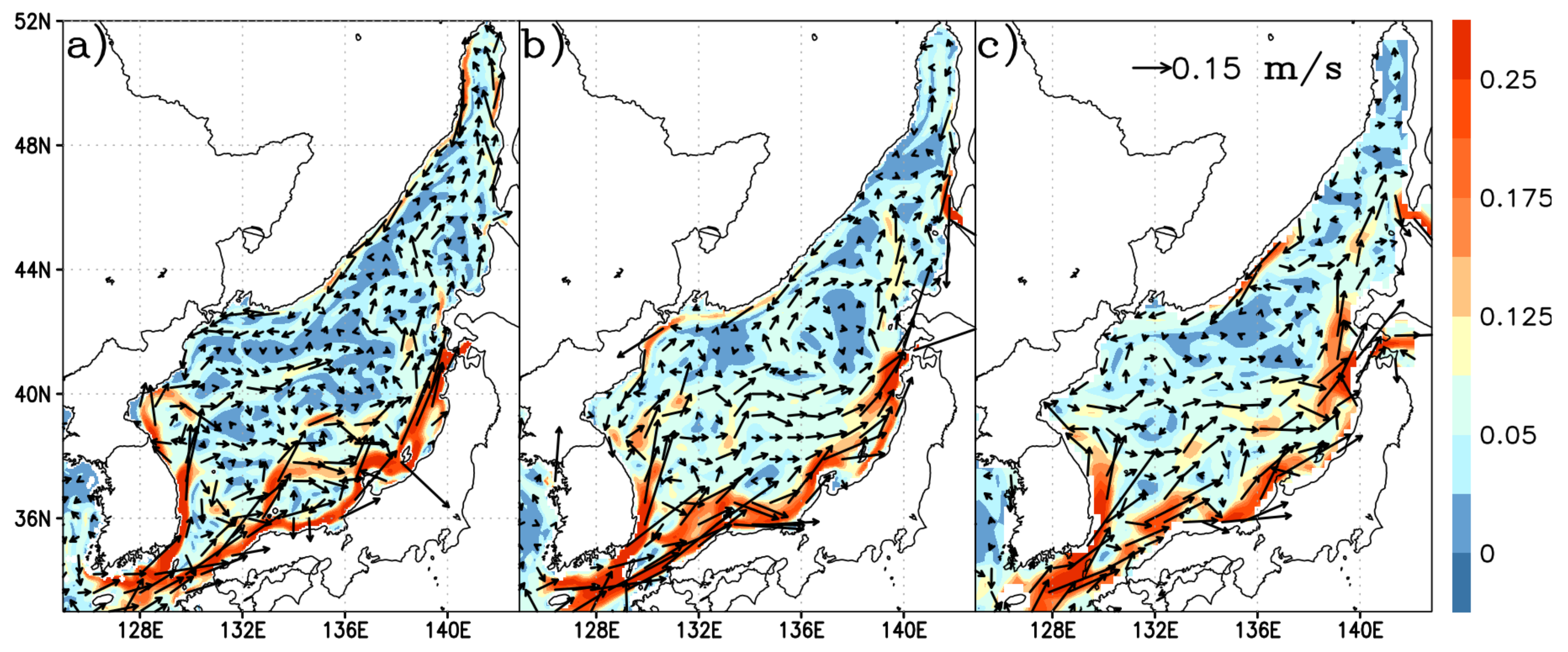
3.2. Simulated Throughflow in the Japan/East Sea
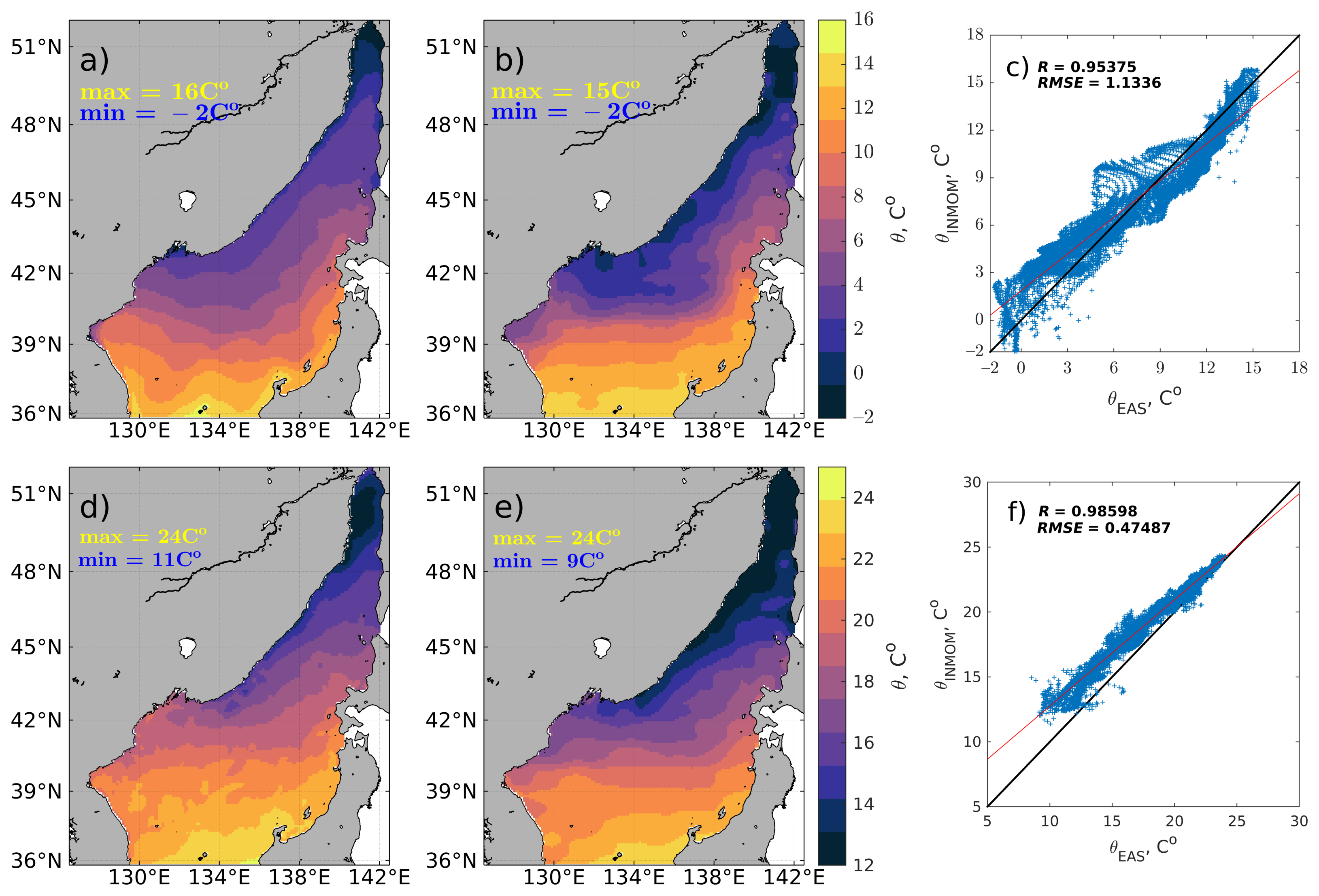
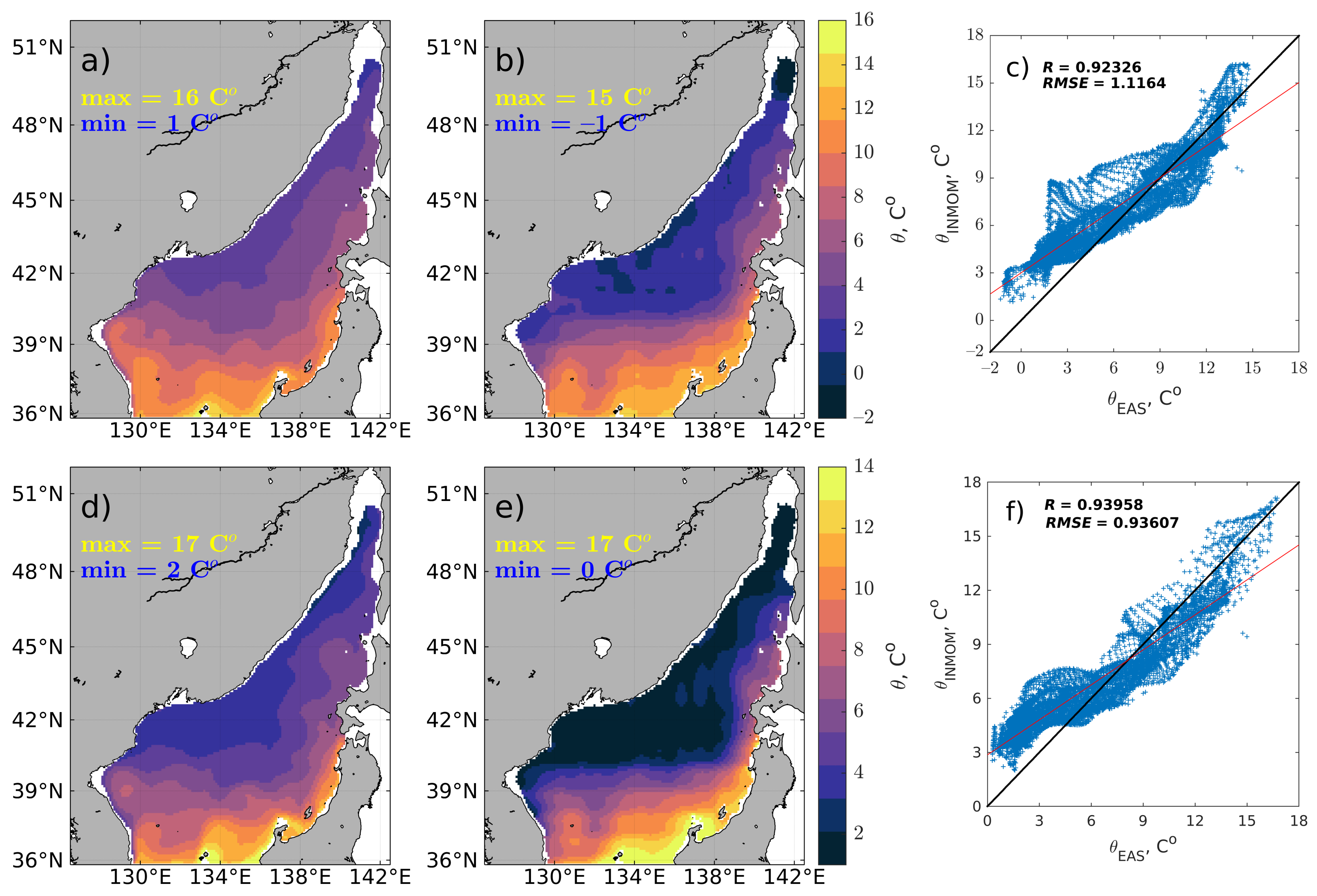
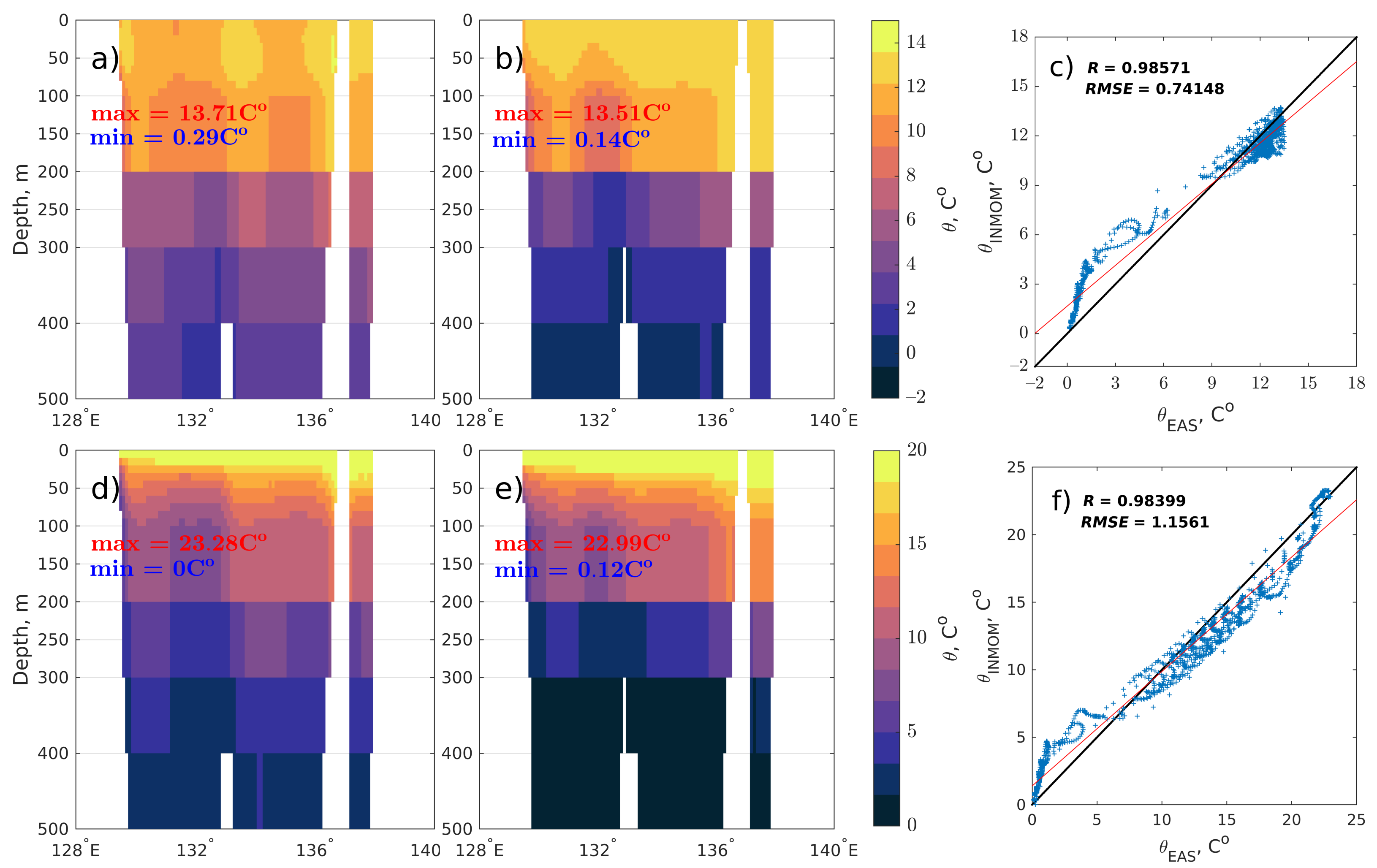
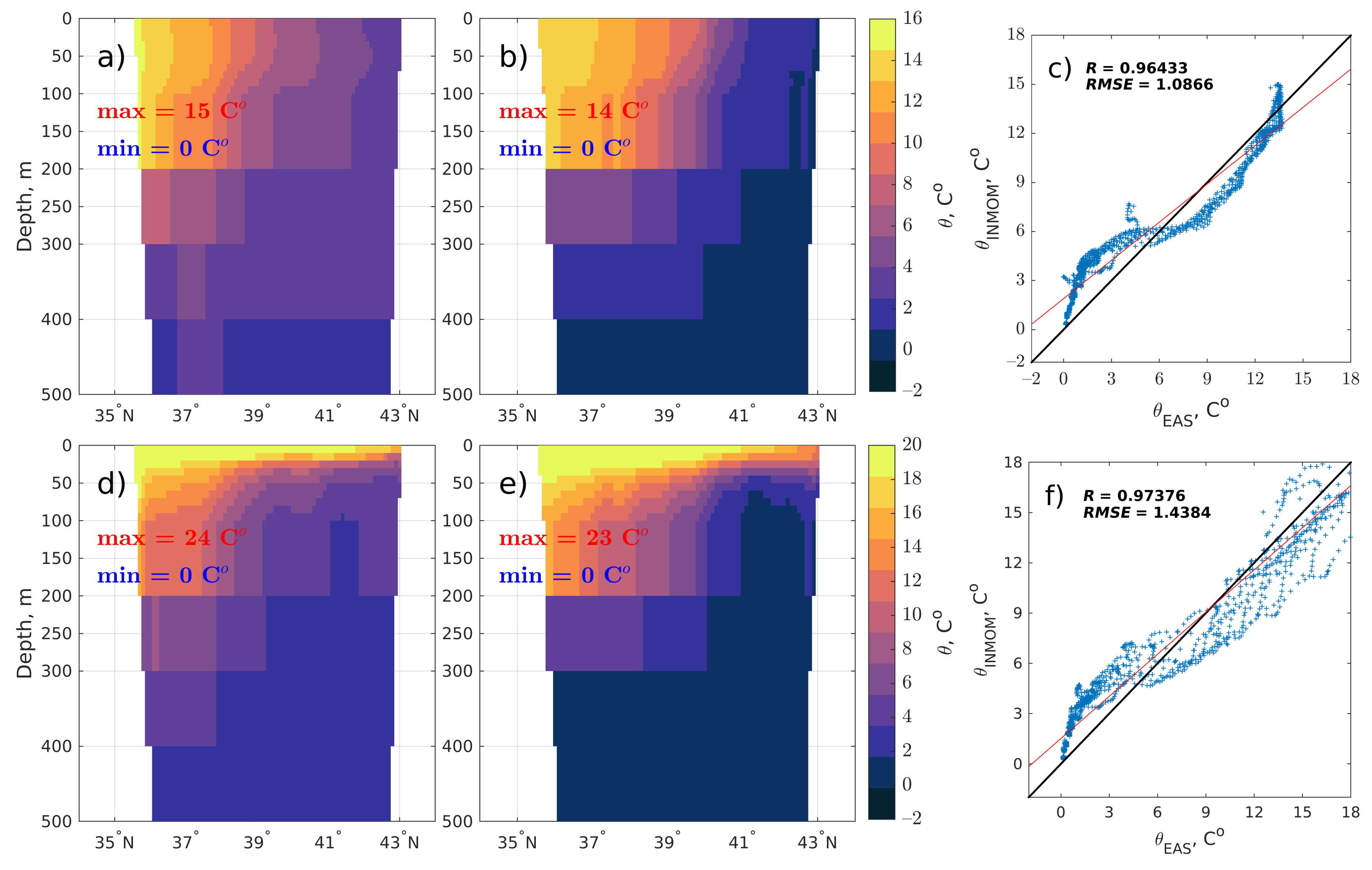
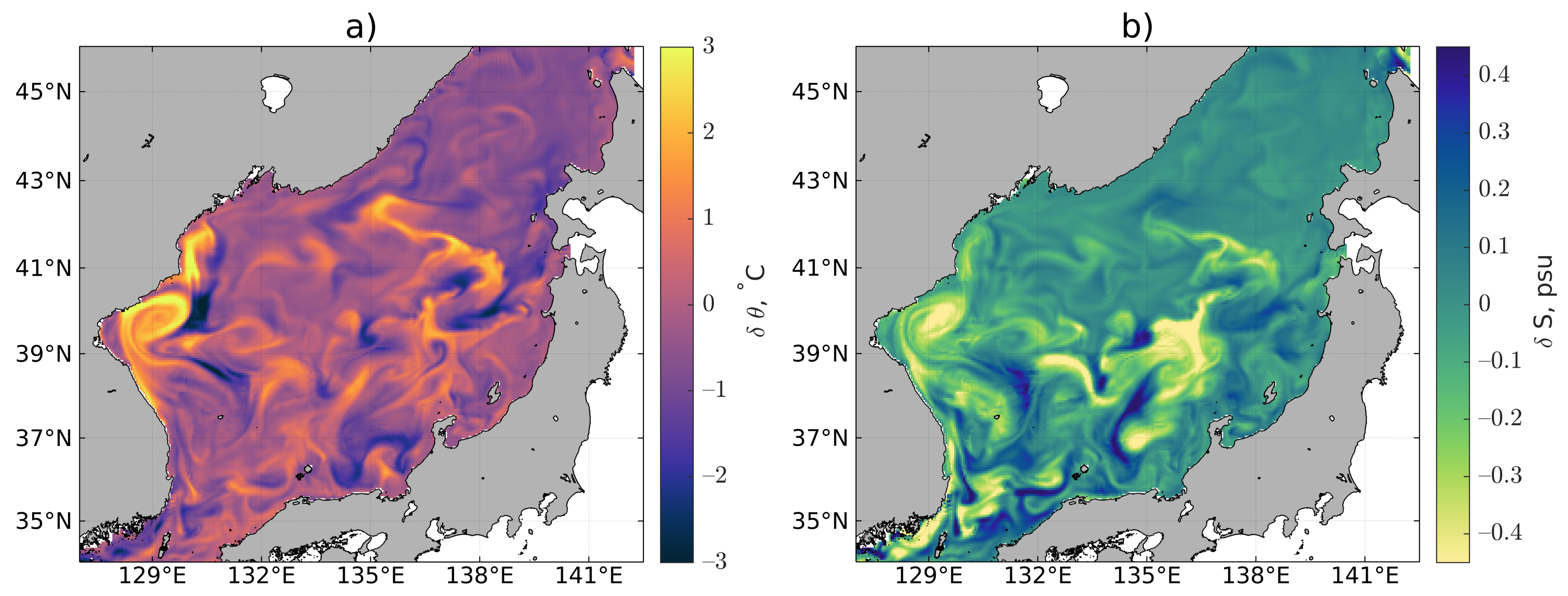
3.3. Simulation-Based Potential Temperature
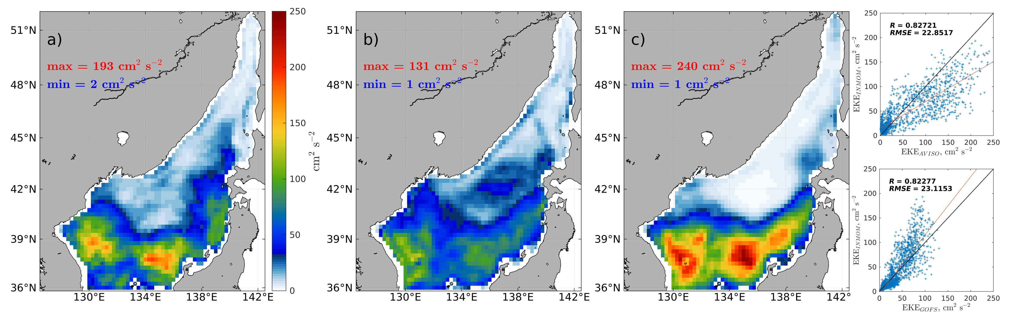
3.4. Simulation-Based Eddy Kinetic Energy
4. Results
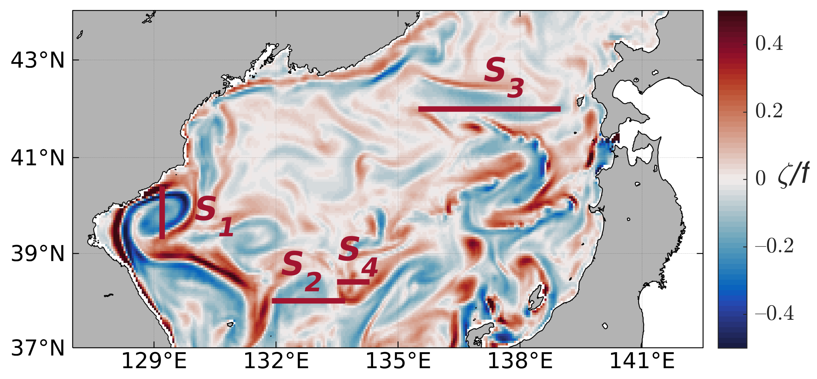
4.1. Simulated Mesoscale Dynamics in the Japan/East Sea
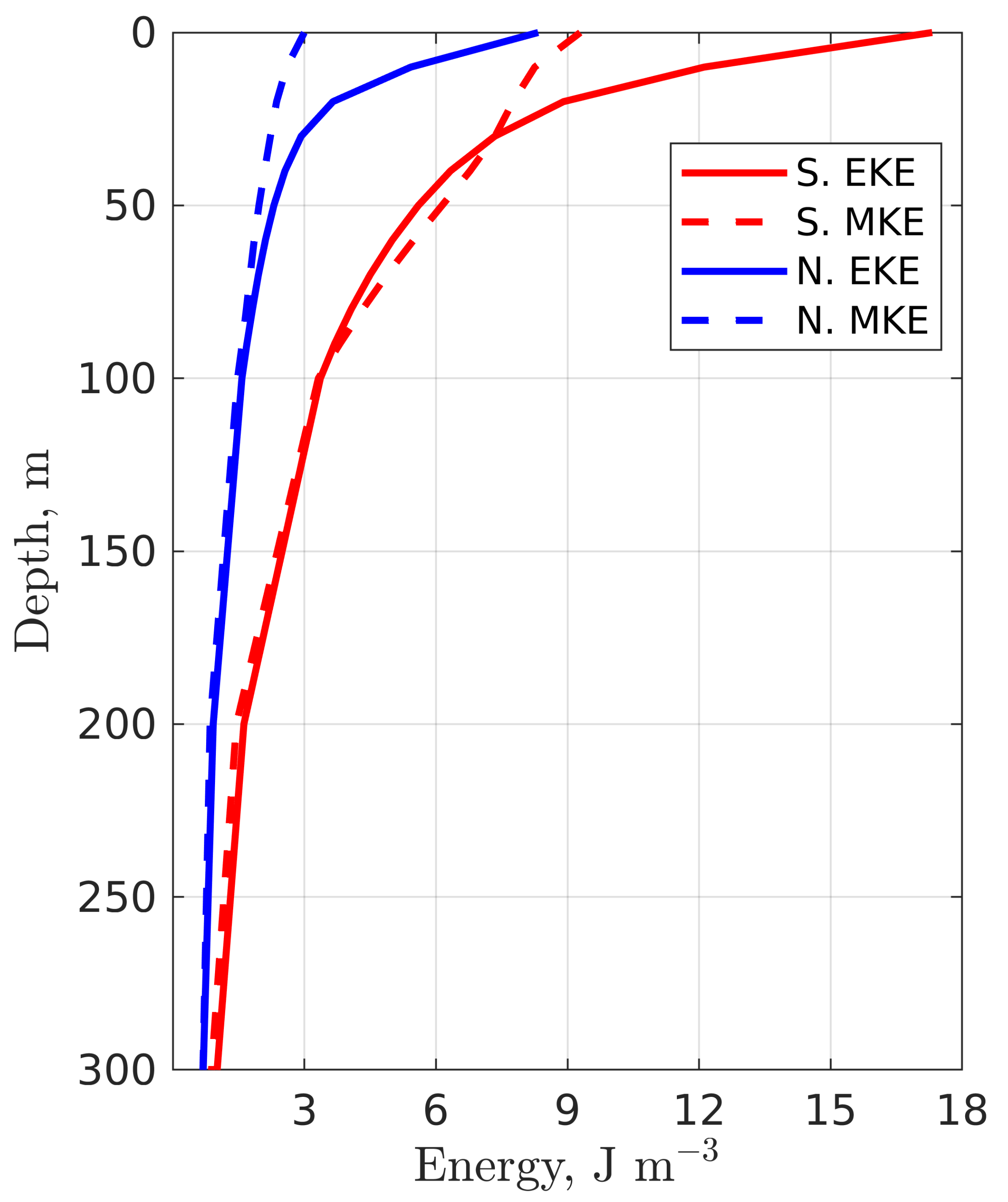
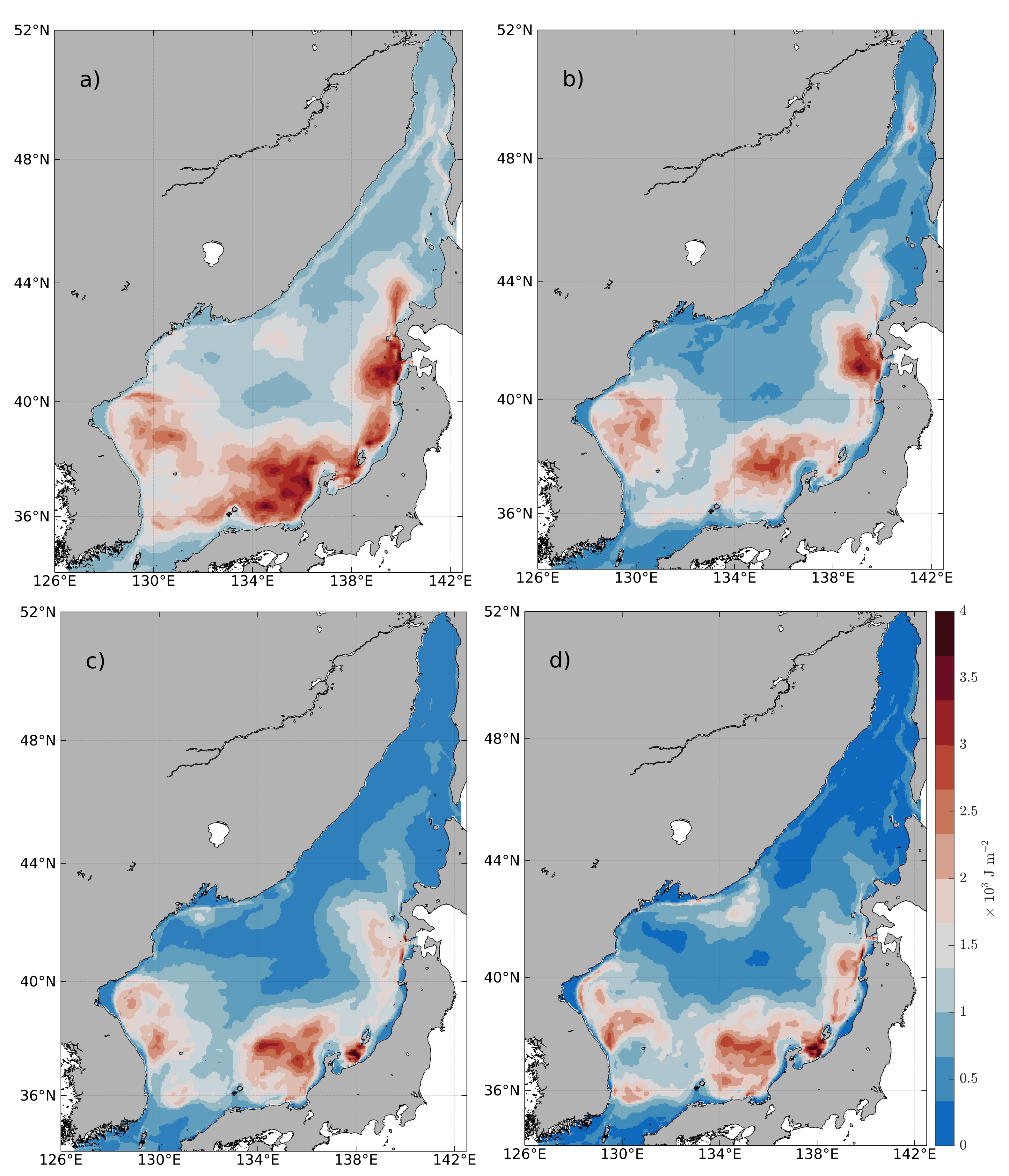
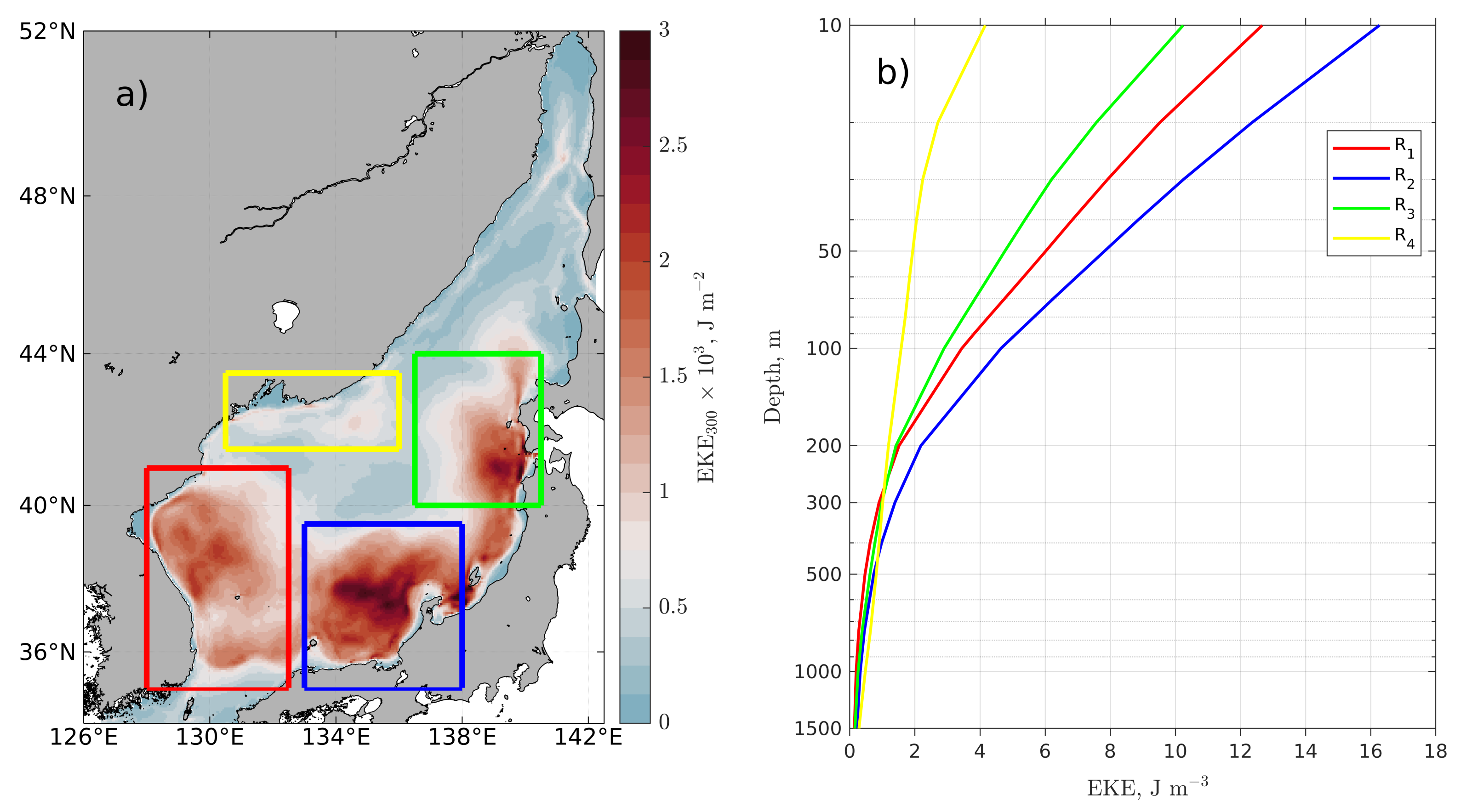
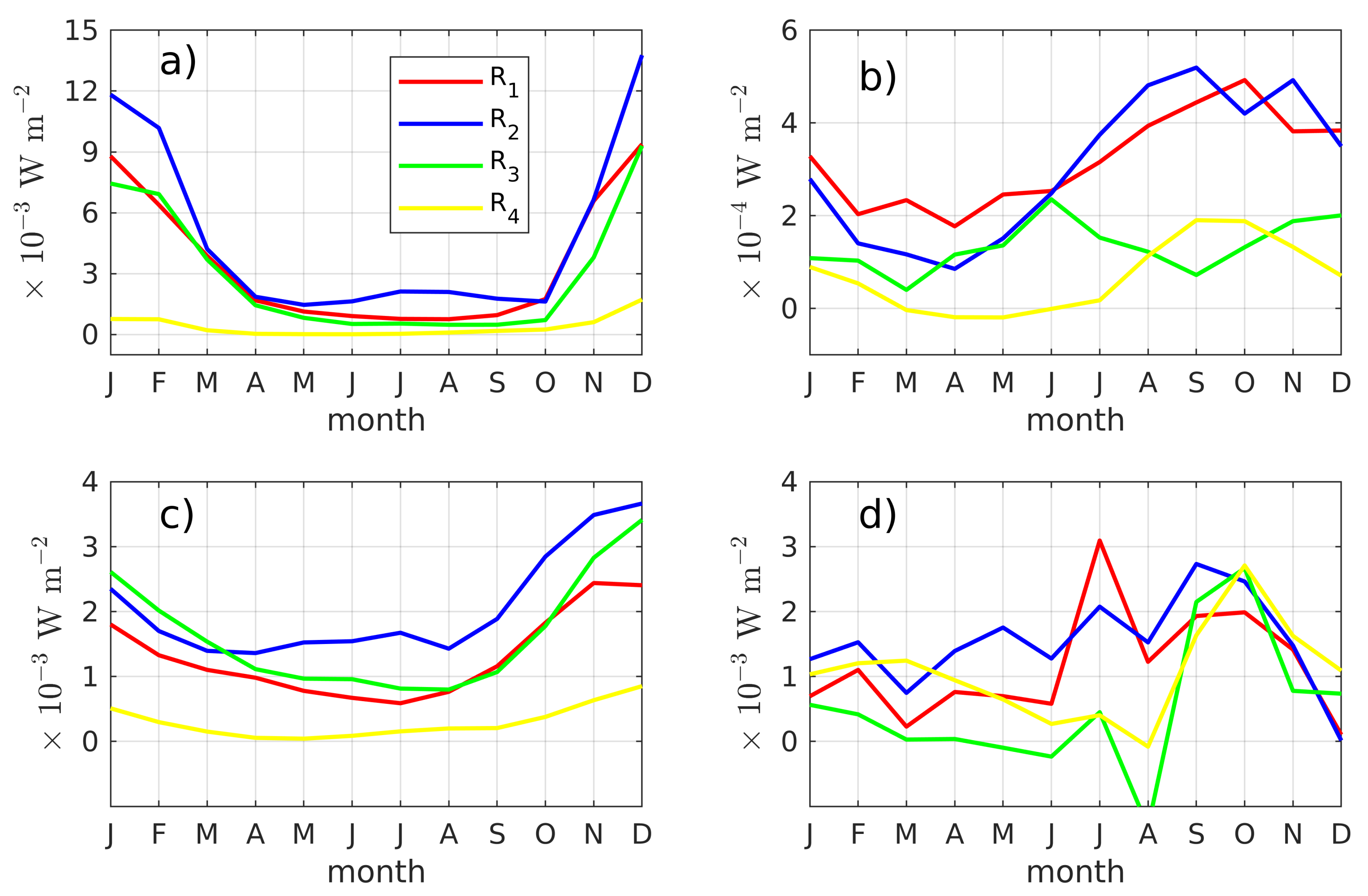
4.2. Eddy Kinetic Energy and Its Sources in the Japan/East Sea
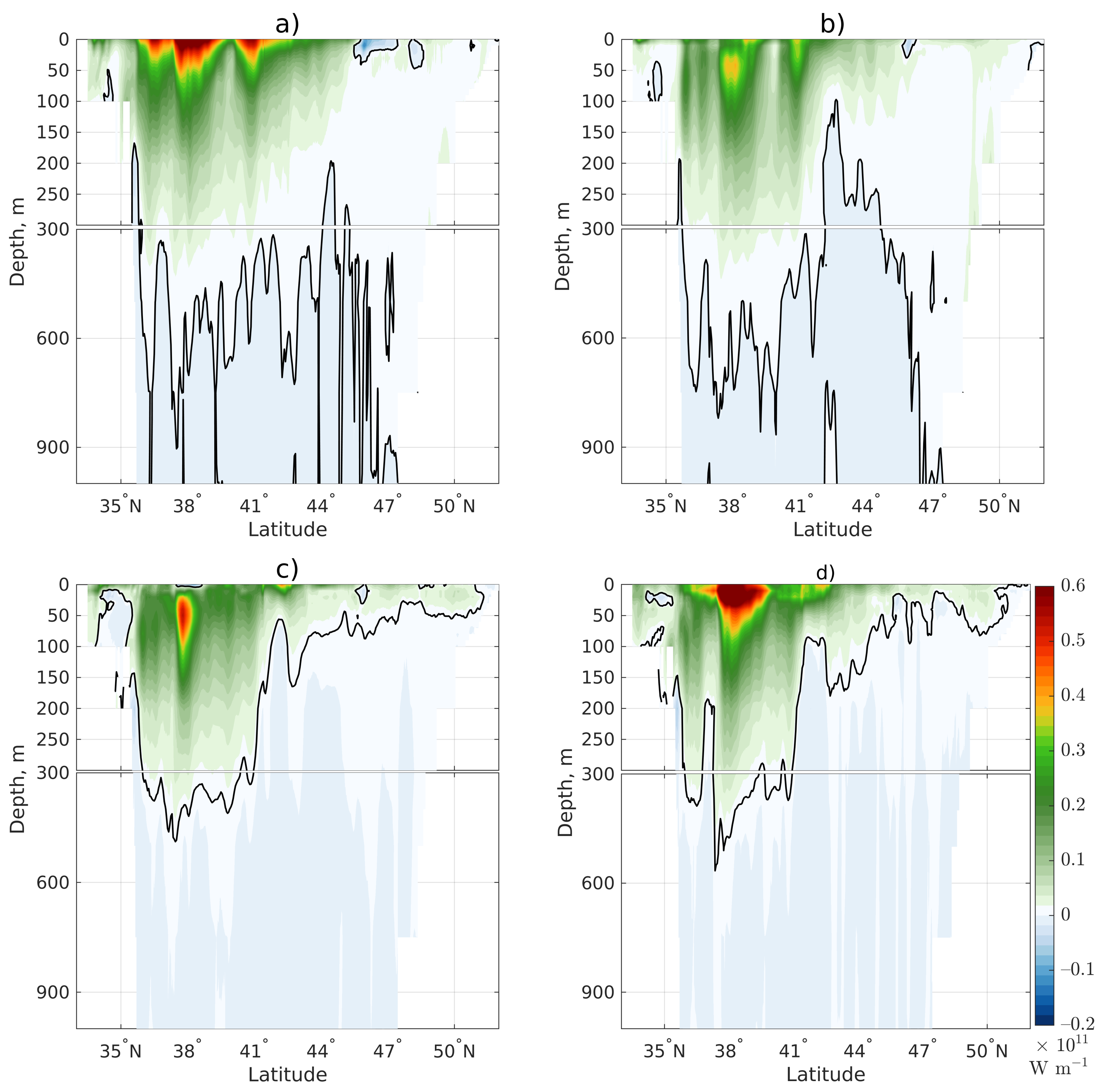
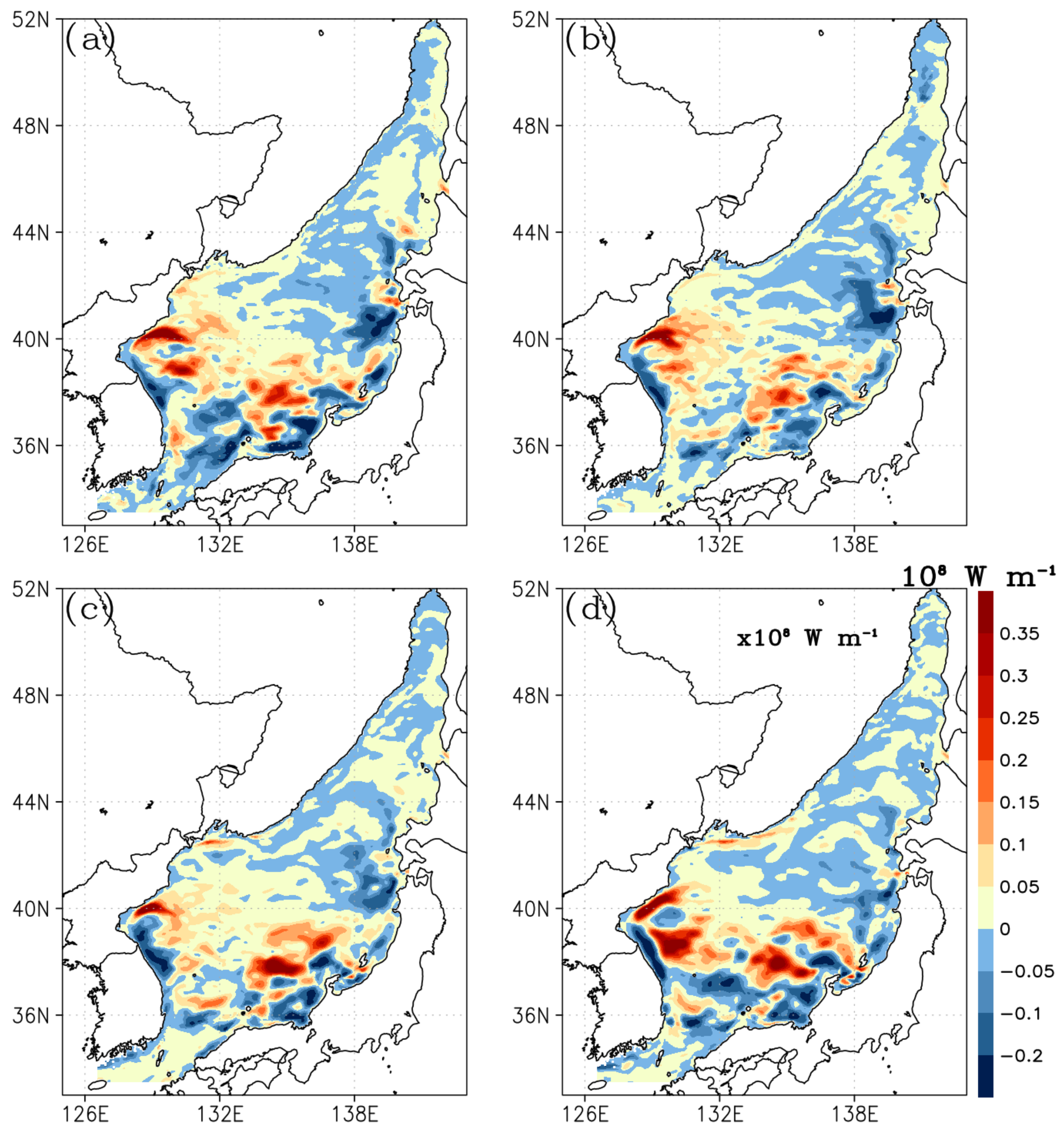
4.3. Horizontal Eddy Heat Transport in the Japan/East Sea
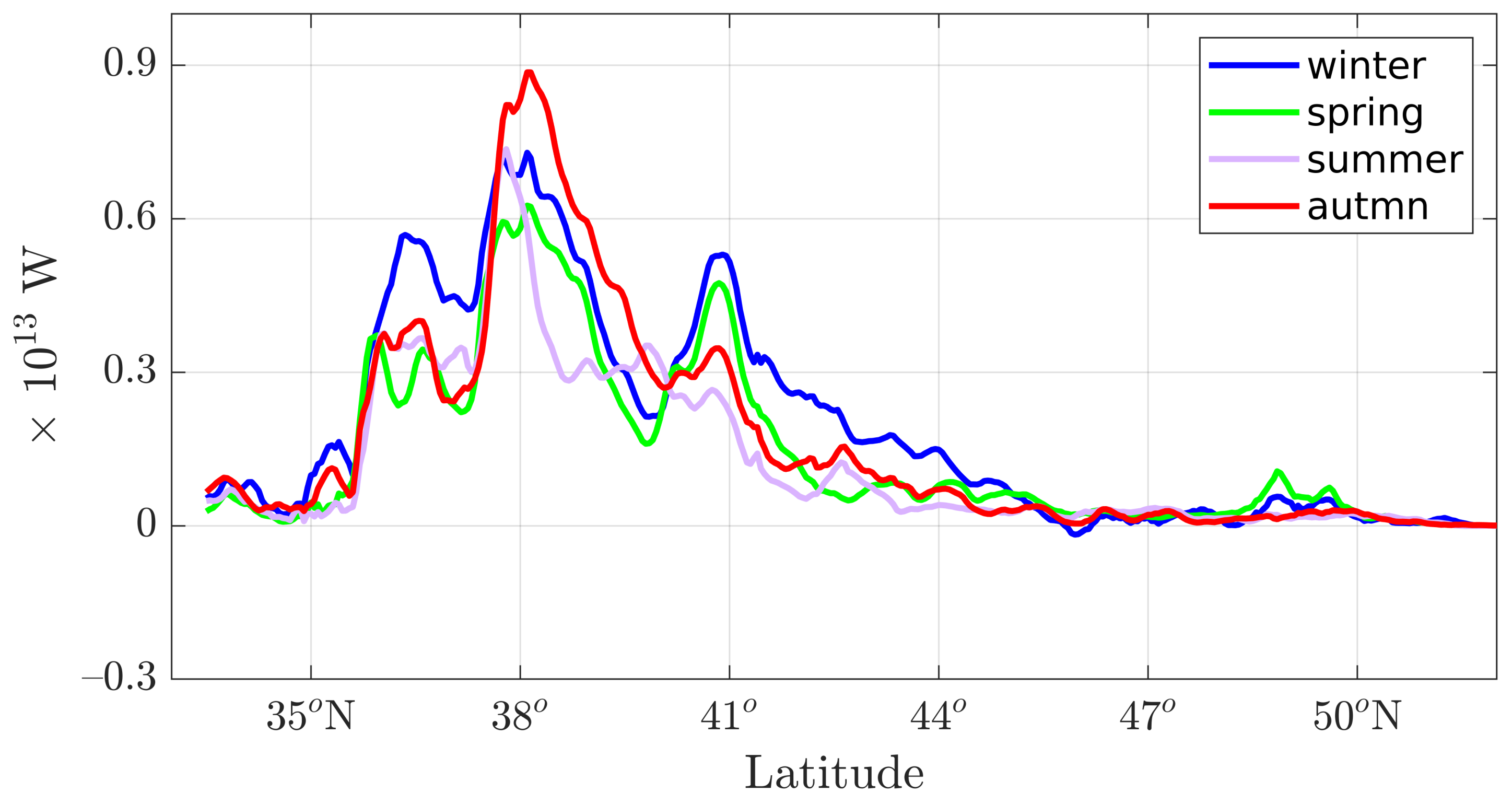
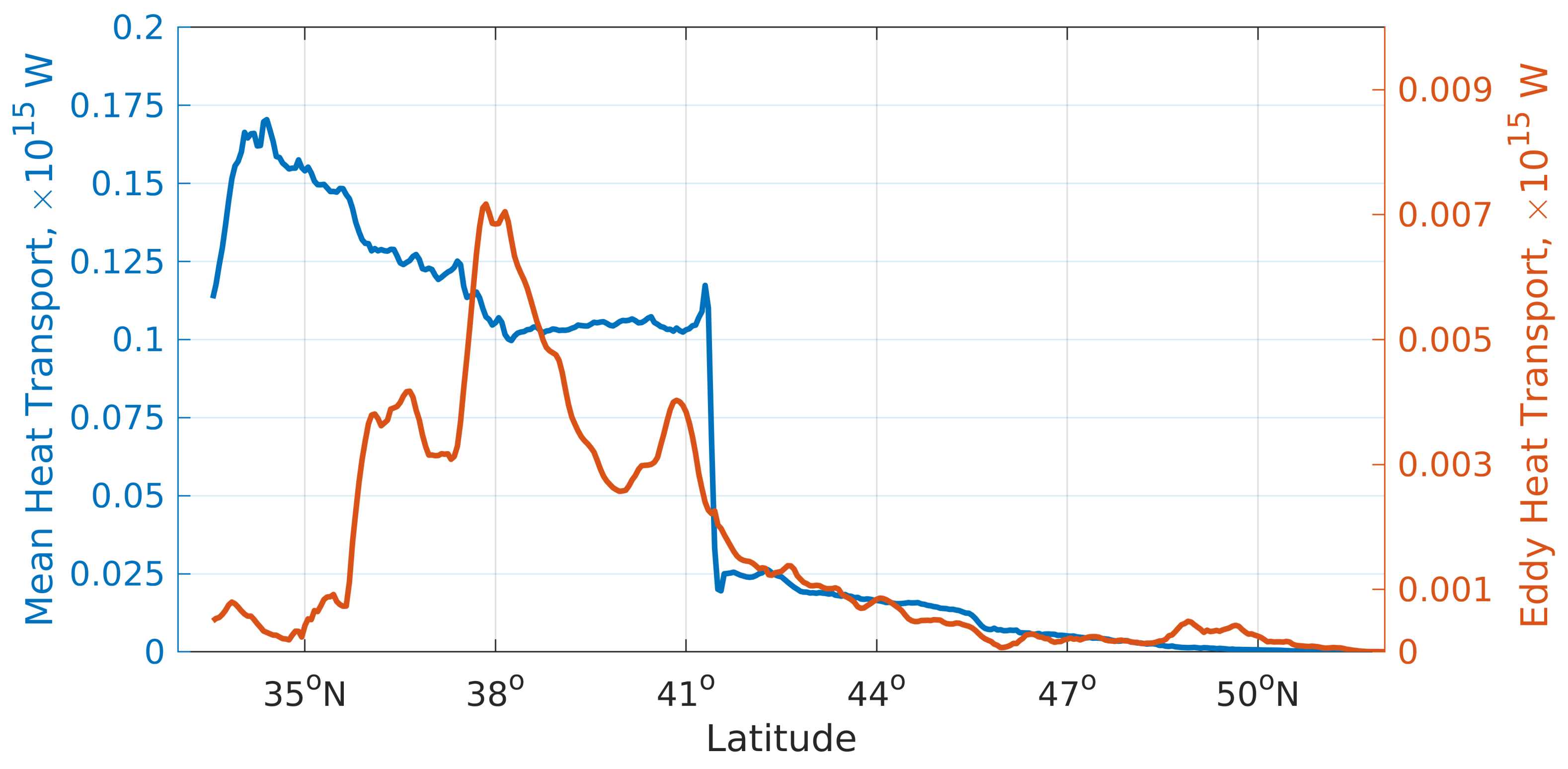
4.3.1. Meridional Heat Transport Induced by the Mesoscale Dynamics in the Japan/East Sea
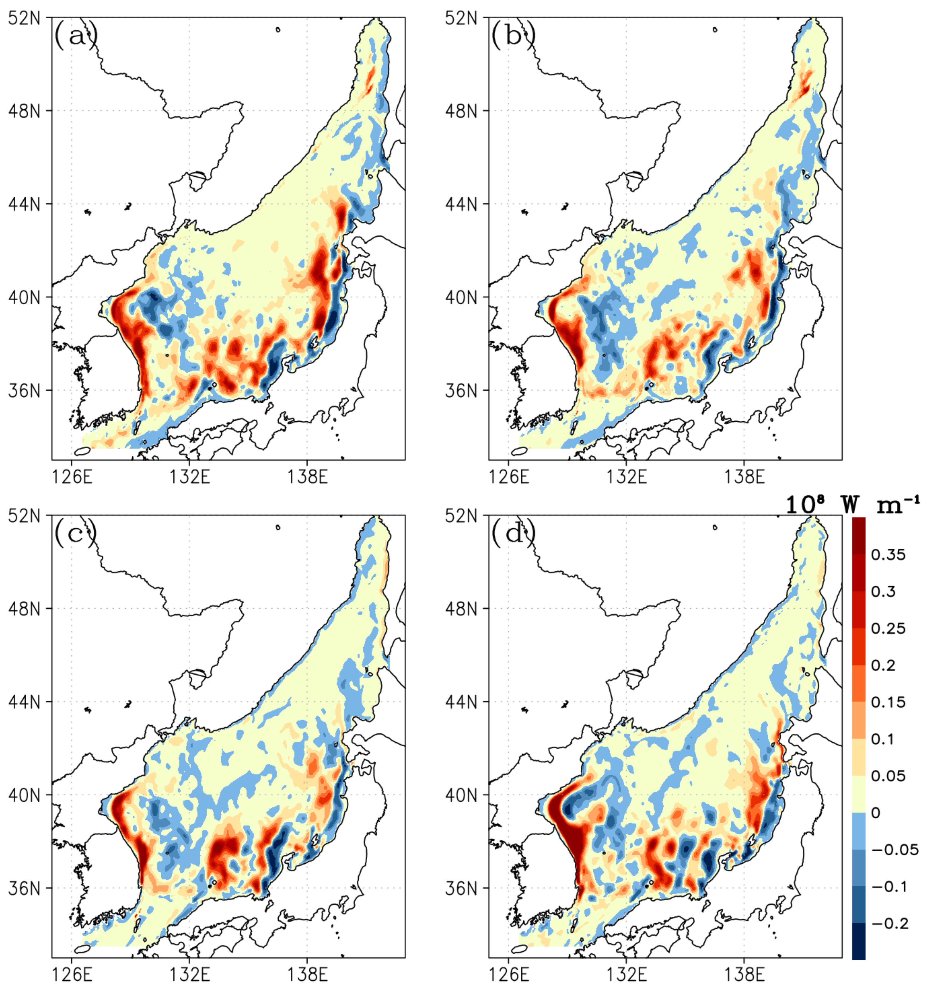
4.3.2. Zonal Eddy Heat Transport in the Japan/East Sea
5. Discussion
6. Conclusions
Author Contributions
Funding
Institutional Review Board Statement
Informed Consent Statement
Data Availability Statement
Conflicts of Interest
References
- Sun, B.; Liu, C.; Wang, F. Global meridional eddy heat transport inferred from Argo and altimetry observations. Sci. Rep. 2019, 9, 1345. [Google Scholar] [CrossRef]
- Roemmich, D.; Gilson, J. Eddy Transport of Heat and Thermocline Waters in the North Pacific: A Key to Interannual/Decadal Climate Variability? J. Phys. Oceanogr. 2001, 31, 675–687. [Google Scholar] [CrossRef]
- Volkov, D.; Lee, T.; Fu, L.L. Eddy-induced meridional heat transport in the ocean. Geophys. Res. Lett. 2008, 35, L20601. [Google Scholar] [CrossRef]
- Jayne, S.; Marotzke, J. The Oceanic Eddy Heat Transport. J. Phys. Oceanogr. 2002, 32, 3328–3345. [Google Scholar] [CrossRef]
- Ushakov, K.; Ibrayev, R. The Role of Eddies in Global Oceanic Meridional Heat Transport. Dokl. Earth Sci. 2019, 486, 554–557. [Google Scholar] [CrossRef]
- Early, J.; Samelson, R.; Chelton, D. The Evolution and Propagation of Quasigeostrophic Ocean Eddies. J. Phys. Oceanogr. 2011, 41, 1535–1555. [Google Scholar] [CrossRef]
- Haigh, M.; Sun, L.; McWilliams, J.; Berloff, P. On eddy transport in the ocean. Part II: The advection tensor. Ocean Model. 2021, 165, 101845. [Google Scholar] [CrossRef]
- Griffies, S.; Winton, M.; Anderson, W.; Benson, R.; Delworth, T.; Dufour, C.; Dunne, J.; Goddard, P.; Morrison, A.; Rosati, A.; et al. Impacts on Ocean Heat from Transient Mesoscale Eddies in a Hierarchy of Climate Models. J. Clim. 2015, 28, 952–977. [Google Scholar] [CrossRef]
- Chelton, D.; Schlax, M.; Samelson, R. Global observations of nonlinear mesoscale eddies. Prog. Oceanogr. 2011, 91, 167–216. [Google Scholar] [CrossRef]
- Zhang, Z.; Wang, W.; Qiu, B. Oceanic mass transport by mesoscale eddies. Science 2014, 345, 322–324. [Google Scholar] [CrossRef]
- von Storch, J.S.; Eden, C.; Fast, I.; Haak, H.; Hernandez-Deckers, D.; Maier-Reimer, E.; Marotzke, J.; Stammer, D. An estimate of the Lorenz energy cycle for the World Ocean based on the 1/10 STORM/NCEP simulation. J. Phys. Oceanogr. 2012, 42, 2185–2205. [Google Scholar] [CrossRef]
- Eden, C.; Boning, C. Sources of Eddy Kinetic Energy in the Labrador Sea. J. Phys. Oceanogr. 2002, 32, 3346–3363. [Google Scholar] [CrossRef]
- Stammer, D. Global Characteristics of Ocean Variability Estimated from Regional TOPEX/POSEIDON Altimeter Measurements. J. Phys. Oceanogr. 1997, 27, 1743–1769. [Google Scholar] [CrossRef]
- Maslo, A.; Azevedo Correia de Souza, J.; Pardo, J. Energetics of the Deep Gulf of Mexico. J. Phys. Oceanogr. 2020, 50, 1655–1675. [Google Scholar] [CrossRef]
- Demyshev, S.; Dymova, O. Numerical analysis of the Black Sea currents and mesoscale eddies in 2006 and 2011. Ocean Dyn. 2018, 68, 1335–1352. [Google Scholar] [CrossRef]
- Shore, J.; Stacey, M.; Wright, D. Sources of Eddy Energy Simulated by a Model of the Northeast Pacific Ocean. J. Phys. Oceanogr. 2008, 38, 2283–2293. [Google Scholar] [CrossRef]
- Ohshima, K.; Wakatsuchi, M. A Numerical Study of Barotropic Instability Associated with the Soya Warm Current in the Sea of Okhotsk. J. Phys. Oceanogr. 1990, 20, 570–584. [Google Scholar] [CrossRef]
- Zhai, X.; Johnson, H.; Marshall, D.; Wunsch, C. On the Wind Power Input to the Ocean General Circulation. J. Phys. Oceanogr. 2012, 42, 1357–1365. [Google Scholar] [CrossRef]
- Stepanov, D.; Diansky, N.; Fomin, V. Eddy energy sources and mesoscale eddies in the Sea of Okhotsk. Ocean Dyn. 2018, 68, 825–845. [Google Scholar] [CrossRef]
- Hallberg, R. Using a resolution function to regulate parameterizations of oceanic mesoscale eddy effects. Ocean Model. 2013, 72, 92–103. [Google Scholar] [CrossRef]
- Stepanov, D. Estimating the Baroclinic Rossby Radius of Deformation in the Sea of Okhotsk. Russ. Meteorol. Hydrol. 2017, 42, 601–606. [Google Scholar] [CrossRef]
- Chang, K.I.; Zhang, C.I.; Park, C.; Kang, D.J.; Ju, S.J.; Lee, S.H.; Wimbush, M. Oceanography of the East Sea (Japan Sea); Springer: Berlin/Heidelberg, Germany, 2016. [Google Scholar] [CrossRef]
- Isoda, Y. Warm eddy movements in the eastern Japan Sea. J. Oceanogr. 1994, 50, 1–15. [Google Scholar] [CrossRef][Green Version]
- Gordon, A.; Giulivi, C.; Lee, C.; Furey, H.; Bower, A.; Talley, L. Japan/East Sea Intrathermocline Eddies. J. Phys. Oceanogr. 2002, 32, 1960–1974. [Google Scholar] [CrossRef]
- Lee, D.K.; Niiler, P. The energetic surface circulation patterns of the Japan/East Sea. Deep Sea Res. Part II Top. Stud. Oceanogr. 2005, 52, 1547–1563. [Google Scholar] [CrossRef]
- Prants, S.; Budyansky, M.; Ponomarev, V.; Uleysky, M. Lagrangian study of transport and mixing in a mesoscale eddy street. Ocean Model. 2011, 38, 114–125. [Google Scholar] [CrossRef]
- Ostrovskii, A.; Stepanov, D.; Kaplunenko, D.; Park, J.H.; Park, Y.G.; Tishchenko, P. Turbulent mixing and its contribution to the oxygen flux in the northwestern boundary current region of the Japan/East Sea, April–October 2015. J. Mar. Syst. 2021, 224, 103619. [Google Scholar] [CrossRef]
- Prants, S.; Uleysky, M.; Budyansky, M. Lagrangian Analysis of Transport Pathways of Subtropical Water to the Primorye Coast. Dokl. Earth Sci. 2018, 481, 1099–1103. [Google Scholar] [CrossRef]
- Lee, K.; Nam, S.; Kim, Y.G. Statistical Characteristics of East Sea Mesoscale Eddies Detected, Tracked, and Grouped Using Satellite Altimeter Data from 1993 to 2017. J. Korean Soc. Oceanogr. 2019, 24, 267–281. [Google Scholar] [CrossRef]
- Hogan, P.; Hurlburt, H. Impact of Upper Ocean–Topographical Coupling and Isopycnal Outcropping in Japan/East Sea Models with1/8° to1/64° Resolution. J. Phys. Oceanogr. 2000, 30, 2535–2561. [Google Scholar] [CrossRef]
- Jacobs, G.; Hogan, P.; Whitmer, K. Effects of Eddy Variability on the Circulation of the Japan/East Sea. J. Oceanogr. 1999, 55, 247–256. [Google Scholar] [CrossRef]
- Na, H.; Kim, K.Y.; Chang, K.; Park, J.; Kim, K.; Minobe, S. Decadal variability of the upper ocean heat content in the East/Japan Sea and its possible relationship to northwestern Pacific variability. J. Geophys. Res. 2012, 117, C02017. [Google Scholar] [CrossRef]
- Yoon, S.T.; Chang, K.; Na, H.; Minobe, S. An east-west contrast of upper ocean heat content variation south of the subpolar front in the East/Japan Sea. J. Geophys. Res. 2016, 121, 6418–6443. [Google Scholar] [CrossRef]
- Moshonkin, S.; Zalesny, V.; Gusev, A. Simulation of the Arctic—North Atlantic Ocean Circulation with a Two-Equation K-Omega Turbulence Parameterization. J. Mar. Sci. Eng. 2018, 6, 95. [Google Scholar] [CrossRef]
- Danabasoglu, G.; Yeager, S.; Kim, W.; Behrens, E.; Bentsen, M.; Bi, D.; Biastoch, A.; Bleck, R.; Böning, C.; Bozec, A.; et al. North Atlantic simulations in Coordinated Ocean-ice Reference Experiments phase II (CORE-II). Part II: Inter-annual to decadal variability. Ocean Model. 2016, 97, 65–90. [Google Scholar] [CrossRef]
- Frey, D.; Morozov, E.; Fomin, V.; Diansky, N.; Tarakanov, R. Regional Modeling of Antarctic Bottom Water Flows in the Key Passages of the Atlantic. J. Geophys. Res. 2019, 124, 8414–8428. [Google Scholar] [CrossRef]
- Stepanov, D. Mesoscale eddies and baroclinic instability over the eastern Sakhalin shelf of the Sea of Okhotsk: A model-based analysis. Ocean Dyn. 2018, 68, 1353–1370. [Google Scholar] [CrossRef]
- Diansky, N.; Stepanov, D.; Fomin, V.; Chumakov, M. Water Circulation Off the Northeastern Coast of Sakhalin during the Passage of Three Types of Deep Cyclones over the Sea of Okhotsk. Russ. Meteorol. Hydrol. 2020, 45, 29–38. [Google Scholar] [CrossRef]
- Stepanov, D.; Diansky, N.; Novotryasov, V. Numerical simulation of water circulation in the central part of the Sea of Japan and study of its long-term variability in 1958–2006. Izv. Atmos. Ocean. Phys. 2014, 50, 73–84. [Google Scholar] [CrossRef]
- Diansky, N.; Stepanov, D.; Gusev, A.; Novotryasov, V. Role of wind and thermal forcing in the formation of the water circulation variability in the Japan/East Sea Central Basin in 1958–2006. Izv. Atmos. Ocean. Phys. 2016, 52, 207–216. [Google Scholar] [CrossRef]
- Stepanov, D.; Ryzhov, E.; Zagumennov, A.; Berloff, P.; Koshel, K. Clustering of Floating Tracer Due to Mesoscale Vortex and Submesoscale Fields. Geophys. Res. Lett. 2020, 47, e2019GL086504. [Google Scholar] [CrossRef]
- Stepanov, D.; Ryzhov, E.; Berloff, P.; Koshel, K. Floating tracer clustering in divergent random flows modulated by an unsteady mesoscale ocean field. Geophys. Astrophys. Fluid Dyn. 2020, 114, 690–714. [Google Scholar] [CrossRef]
- Ohshima, K.; Simizu, D.; Ebuchi, N.; Morishima, S.; Kashiwase, H. Volume, Heat, and Salt Transports through the Soya Strait and Their Seasonal and Interannual Variations. J. Phys. Oceanogr. 2017, 47, 999–1019. [Google Scholar] [CrossRef]
- Chelton, D.; de Szoeke, R.; Schlax, M. Geographical Variability of the First Baroclinic Rossby Radius of Deformation. J. Phys. Oceanogr. 1998, 28, 433–460. [Google Scholar] [CrossRef]
- Amante, C.; Eakins, B. ETOPO1 1 Arc-Minute Global Relief Model: Procedures, Data Sources and Analysis; Report, NOAA Technical Memorandum NESDIS NGDC-24; NOAA: Silver Spring, MD, USA, 2009. [CrossRef]
- Pacanowski, R.; Philander, S. Parameterization of Vertical Mixing in Numerical Models of Tropical Oceans. J. Phys. Oceanogr. 1981, 11, 1443–1451. [Google Scholar] [CrossRef]
- Large, W.; Yeager, S. The global climatology of an interannually varying air-sea flux data set. J. Clim. 2009, 33, 341–364. [Google Scholar] [CrossRef]
- Straub, D.; Duhaut, T. Wind Stress Dependence on Ocean Surface Velocity: Implications for Mechanical Energy Input to Ocean Circulation. J. Phys. Oceanogr. 2006, 36, 202–211. [Google Scholar] [CrossRef]
- Dee, D.; Uppala, S.; Simmons, A.; Berrisford, P.; Poli, P.; Kobayashi, S.; Andrae, U.; Balmaseda, M.; Balsamo, G.; Bauer, P.; et al. The ERA-Interim reanalysis: Configuration and performance of the data assimilation system. Q. J. Roy. Meteor. Soc. 2011, 137, 553–597. [Google Scholar] [CrossRef]
- Yakovlev, N. Reproduction of the large-scale state of water and sea ice in the Arctic Ocean in 1948–2002: Part I. Numerical model. Izv. Atmos. Ocean. Phys. 2009, 45, 357–371. [Google Scholar] [CrossRef]
- Zweng, M.; Reagan, J.; Antonov, J.; Locarnini, R.; Mishonov, A.; Boyer, T.; Garcia, H.; Baranova, O.; Johnson, D.; Seidov, D.; et al. World Ocean Atlas 2013, Volume 2: Salinity; NOAA: Silver Spring, MD, USA, 2013.
- Locarnini, R.; Mishonov, A.; Antonov, J.; Boyer, T.; Garcia, H.; Baranova, O.; Zweng, M.; Paver, C.; Reagan, J.; Johnson, D.; et al. World Ocean Atlas 2013, Volume 1: Temperature; NOAA: Silver Spring, MD, USA, 2013.
- Cummings, J. Operational multivariate ocean data assimilation. Q. J. Roy. Meteor. Soc. 2005, 131, 3583–3604. [Google Scholar] [CrossRef]
- Johnson, D.; Boyer, T.; Seidov, D.; Mishonov, A. Regional Climatology of the East Asian Seas: An Introduction; NOAA: Silver Spring, MD, USA, 2015. [CrossRef]
- Fukudome, K.; Yoon, J.; Ostrovskii, A.; Takikawa, T.; Han, I.S. Seasonal Volume Transport Variation in the Tsushima Warm Current through the Tsushima Straits from 10 Years of ADCP Observations. J. Oceanogr. 2010, 66, 539–551. [Google Scholar] [CrossRef]
- Ito, T.; Togawa, O.; Ohnishi, M.; Isoda, Y.; Nakayama, T.; Shima, S.; Kuroda, H.; Iwahashi, M.; Sato, C. Variation of velocity and volume transport of the Tsugaru Warm Current in the winter of 1999–2000. Geophys. Res. Lett. 2003, 30, 1678. [Google Scholar] [CrossRef]
- Saveliev, A.; Danchenkov, M.; Hong, G.H. Volume Transport through the La-Perouse (Soya) Strait between the East Sea (Sea of Japan) and the Sea of Okhotsk. Ocean Polar Res. 2002, 24, 147–152. [Google Scholar] [CrossRef]
- Kim, T.; Yoon, J. Seasonal variation of upper layer circulation in the northern part of the East/Japan Sea. Cont. Shelf Res. 2010, 30, 1283–1301. [Google Scholar] [CrossRef]
- Yoon, J.; Abe, K.; Ogata, T.; Wakamatsu, Y. The effects of wind-stress curl on the Japan/East Sea circulation. Deep Sea Res. Part II Top. Stud. Oceanogr. 2005, 52, 1827–1844. [Google Scholar] [CrossRef]
- Qiu, B. Seasonal Eddy Field Modulation of the North Pacific Subtropical Countercurrent: TOPEX/Poseidon Observations and Theory. J. Phys. Oceanogr. 1999, 29, 2471–2486. [Google Scholar] [CrossRef]
- Chang, K.; Teague, W. Circulation and currents in the southwestern East/Japan Sea: Overview and review. Prog. Oceanogr. 2004, 61, 105–156. [Google Scholar] [CrossRef]
- Ferrari, R.; Wunsch, C. Ocean Circulation Kinetic Energy: Reservoirs, Sources, and Sinks. Annu. Rev. Fluid Mech. 2009, 41, 253–282. [Google Scholar] [CrossRef]
- Pedlosky, J. Geophysical Fluid Dynamics; Springer: New York, NY, USA, 1987. [Google Scholar] [CrossRef]
- Qiu, B.; Chen, S. Eddy-Induced Heat Transport in the Subtropical North Pacific from Argo, TMI, and Altimetry Measurements. J. Phys. Oceanogr. 2005, 35, 458–473. [Google Scholar] [CrossRef]
- Ding, R.; Xuan, J.; Zhang, T.; Zhou, L.; Zhou, F.; Meng, Q.; Kang, I. Eddy-Induced Heat Transport in the South China Sea. J. Phys. Oceanogr. 2021, 51, 2329–2349. [Google Scholar] [CrossRef]
- Ladychenko, S.; Lobanov, V. Mesoscale eddies in the area of Peter the Great Bay according to satellite data. Izv. Atmos. Ocean. Phys. 2014, 49, 939–951. [Google Scholar] [CrossRef]
- Marshall, J.; Shutts, G. A Note on Rotational and Divergent Eddy Fluxes. J. Phys. Oceanogr. 1981, 11, 1677–1680. [Google Scholar] [CrossRef]
- Lee, D.; Niiler, P.; Lee, S.; Kim, K.; Lie, H. Energetics of the surface circulation of the Japan/East Sea. J. Geophys. Res. Oceans 2000, 105, 19561–19573. [Google Scholar] [CrossRef]
- Yoon, J.H.; Kim, Y.J. Review on the seasonal variation of the surface circulation in the Japan/East Sea. J. Mar. Syst. 2009, 78, 226–236. [Google Scholar] [CrossRef]
- Kim, T.; Jo, H.J.; Moon, J.H. Occurrence and Evolution of Mesoscale Thermodynamic Phenomena in the Northern Part of the East Sea (Japan Sea) Derived from Satellite Altimeter Data. Remote Sens. 2021, 13, 1071. [Google Scholar] [CrossRef]
- Isobe, A.; Mitsuru, A.; Toshiteru, W.; Tomoharu, S.; Shigehiko, S.; Atsuyoshi, M. Freshwater and temperature transports through the Tsushima-Korea Straits. J. Oceanogr. 2002, 107, 3065. [Google Scholar] [CrossRef]
- Seo, G.H.; Cho, Y.K.; Choi, B.J. Variations of heat transport in the northwestern Pacific marginal seas inferred from high-resolution reanalysis. Prog. Oceanogr. 2014, 121, 98–108. [Google Scholar] [CrossRef]
- Park, J.; Lim, B. A new perspective on origin of the East Sea Intermediate Water: Observations of Argo floats. Prog. Oceanogr. 2018, 160, 213–224. [Google Scholar] [CrossRef]


| Model domain | 123 E–147.25 E, 28.3 N–52.12 N |
| Topography | ETOPO1 |
| Horizontal resolution | |
| Vertical resolution | 25 -levels |
| Hindcast period | 1979–2011 |
| Mixing technique | Laplace-like operator |
| Heat and salt lateral | |
| diffusivity | 5 m s |
| Lateral harmonic viscosity | 10 m s |
| Vertical mixing | Pacanowski–Philander method |
| parameterization | |
| Vertical diffusivity of salt | 10 m s |
| and heat | |
| Vertical viscosity | 10 m s |
| Convective mixing is | |
| parameterized by enhanced | |
| vertical diffusivity | 0.005 m s |
| and vertical viscosity | 0.025 m s |
| Dataset (Period) | Korea/Tsushima Strait, Sv | Tsugaru Strait, Sv | Soya Strait, Sv |
|---|---|---|---|
| INMOM-ERA Int. (1990–2010) | 2.58 | 2.04 | 0.17 |
| Fukudome et al. [55](1997–2007) | 2.65 | – | – |
| Ito et al. [56] (1999–2000) | – | 1.51 | – |
| Ohshima et al. [43] (2003–2015) | – | – | 0.91 |
| Saveliev et al. [57](1975–1988) | – | – | 0.61 |
| GOFS3.1 (1994–2010) | 2.58 | 1.76 | 0.63 |
Publisher’s Note: MDPI stays neutral with regard to jurisdictional claims in published maps and institutional affiliations. |
© 2021 by the authors. Licensee MDPI, Basel, Switzerland. This article is an open access article distributed under the terms and conditions of the Creative Commons Attribution (CC BY) license (https://creativecommons.org/licenses/by/4.0/).
Share and Cite
Stepanov, D.; Fomin, V.; Gusev, A.; Diansky, N. Mesoscale Dynamics and Eddy Heat Transport in the Japan/East Sea from 1990 to 2010: A Model-Based Analysis. J. Mar. Sci. Eng. 2022, 10, 33. https://doi.org/10.3390/jmse10010033
Stepanov D, Fomin V, Gusev A, Diansky N. Mesoscale Dynamics and Eddy Heat Transport in the Japan/East Sea from 1990 to 2010: A Model-Based Analysis. Journal of Marine Science and Engineering. 2022; 10(1):33. https://doi.org/10.3390/jmse10010033
Chicago/Turabian StyleStepanov, Dmitry, Vladimir Fomin, Anatoly Gusev, and Nikolay Diansky. 2022. "Mesoscale Dynamics and Eddy Heat Transport in the Japan/East Sea from 1990 to 2010: A Model-Based Analysis" Journal of Marine Science and Engineering 10, no. 1: 33. https://doi.org/10.3390/jmse10010033
APA StyleStepanov, D., Fomin, V., Gusev, A., & Diansky, N. (2022). Mesoscale Dynamics and Eddy Heat Transport in the Japan/East Sea from 1990 to 2010: A Model-Based Analysis. Journal of Marine Science and Engineering, 10(1), 33. https://doi.org/10.3390/jmse10010033