Multi-Dimensional Monitoring of Agricultural Drought at the Field Scale

Abstract

The causes of agricultural drought are complex, and its actual occurrence process is often characterized by rapid onset in terms of time and small scale in terms of space. Monitoring agricultural drought using satellite remote sensing with low spatial resolution makes it difficult to accurately capture the details of small-scale drought events. High-resolution satellite remote sensing has relatively long revisit cycles, making it difficult to capture the rapid evolution of drought conditions. Furthermore, the occurrence of agricultural drought is linked to multiple factors including precipitation, evapotranspiration, soil properties, and crop physiological characteristics. Consequently, relying on a single variable or indicator is insufficient for multidimensional monitoring of agricultural drought. This study takes Hebi City, Henan Province as the research area. It uses Sentinel-1 satellite data (HV, VV), Sentinel-2 data (NDVI, B2, B11), elevation, slope, aspect, and GPM precipitation data from 2019 to 2024 as independent variables. Three machine learning algorithms—Random Forest (RF), Random Forest-Recursive Feature Elimination (RF-RFE), and eXtreme Gradient Boosting (XGBoost)—were employed to construct a multi-dimensional agricultural drought monitoring model at the field scale. Additionally, the study verified the sensitivity of different environmental variables to agricultural drought monitoring and analyzed the accuracy performance of different machine learning algorithms in agricultural drought monitoring. The research results indicate that under the condition of full-factor input, all three models exhibit the optimal predictive performance. Among them, the XGBoost model performs the best, with the smallest Relative Root Mean Square Error (RRMSE) of 0.45 and the highest Correlation Coefficient (R) of 0.79. The absence of Digital Elevation Model (DEM) data impairs the models’ ability to capture the patterns of key features, which in turn leads to a reduction in predictive accuracy. Meanwhile, there is a significant correlation between model performance and sample size. Ultimately, the constructed XGBoost model takes the lead with an accuracy of 89%, while the accuracies of Random Forest (RF) and Random Forest-Recursive Feature Elimination (RF-RFE) are 88% and 86%, respectively. Based on these three drought monitoring models, this study further monitored a drought event that occurred in Hebi City in 2023, presented the spatiotemporal distribution of agricultural drought in Hebi City, and applied the Mann–Kendall test for time series analysis, aiming to identify the abrupt change process of agricultural drought. Meanwhile, on the basis of the research results, the feasibility of verifying drought occurrence using irrigation signals was discussed, and the potential reasons for the significantly lower drought occurrence probability in the western mountainous areas of the study region were analyzed.

1. Introduction

Extreme drought events are occurring with increasing frequency, exerting significant impacts on ecological environments, agricultural production, and socio-economic development. Depending on the subject of study, drought can be categorized into four principal types: meteorological drought, agricultural drought, hydrological drought, and socio-economic drought [1]. Among these, agricultural drought refers to a condition where, during the crop growing period, insufficient or unevenly distributed precipitation leads to severe soil moisture deficit. This deficit affects crop growth and development, causing crop damage, yield reduction, or even total crop failure [2]. Hence, identifying effective methods for monitoring agricultural drought has long been a subject of significant research interest in various disciplines, including water sciences, agricultural sciences, and geographic information science.

The mainstream technical methods in the current field of agricultural drought monitoring can be categorized into three major types: monitoring methods based on meteorological data and mechanistic models, those based on ground sensors and Internet of Things (IoT) technology, and monitoring methods based on satellite remote sensing data that have developed rapidly in the past decade. From the perspective of technological development history, monitoring methods based on meteorological data and mechanistic models represent the earliest applied technical system. Among these, studies centered on crop water balance models have established a mature theoretical framework and application paradigm. For instance, Zhou et al. [3] modeled the soil water balance by integrating the Hydrus-1D and CropWat models, and assessed irrigation performance and water use efficiency, which in turn provided a methodology for water-saving management in the Heihe River Basin of Gansu Province. In another study, Mathobo et al. [4] utilized crop-specific parameters for dry beans to calibrate and validate a Soil Water Balance (SWB) model. Their results demonstrated a strong agreement between the simulated and measured values for leaf area index, total dry weight, harvestable dry weight, and soil water deficit, indicating that the calibrated model can serve as an effective irrigation scheduling tool. In the application of crop water balance models, most models-especially simplified models commonly used at the regional scale-generally adopt the assumptions of “homogeneous soil” and “average crop coefficient” to simplify calculations In real-world scenarios, however, significant spatial heterogeneity in soils exists due to topography, parent material, and farming practices, while actual crop water requirements often deviate substantially from the “standard crop coefficient” owing to pests, diseases, variations in fertility, and planting density. These micro-scale variations are often masked by the averaging assumptions in models. Consequently, models generally struggle to accurately delineate “within-field variability” in regional field-scale studies [5,6,7]. Although some complex mechanistic models, supported by detailed micro-scale observations, can partially capture these differences at the plot scale, their spatial resolution is limited by the density of meteorological stations. Furthermore, their strong dependency on parameters, which are challenging to calibrate, continues to constrain their general applicability. It can thus be seen that the results of current agricultural drought monitoring based on meteorological data and mechanistic models have limited guiding value for precision irrigation and local disaster relief efforts.

With the continuous advancement of automated sensors and wireless network technologies, the measurement accuracy and operational cost of sensors have entered a new tier [8,9]. Meanwhile, their capabilities of all-weather continuous monitoring, real-time data collection, and transmission have significantly enhanced the dynamic capture of key agricultural drought parameters (e.g., soil moisture content, crop canopy temperature) [10], driving agricultural drought monitoring research based on ground sensors and IoT technology toward a vigorous development trend characterized by high efficiency and precision. In current practical applications, remote sensing monitoring continues to dominate agricultural drought monitoring due to its extensive coverage, multi-temporal dynamic observation capabilities, and mature operational application systems. Its technical paradigms and data products enjoy high industry recognition. However, the precision advantages of ground sensors and IoT technologies are gradually emerging. As equipment costs continue to decrease, multi-source data fusion technologies mature, and operational maintenance systems improve, their application potential will be progressively realized. The current high deployment costs of sensors and the lack of continuous spatial monitoring continue to constrain the application and promotion of sensor stations in agricultural drought monitoring.

Satellite remote sensing data are primarily employed to monitor agricultural drought through methods such as deriving soil moisture content, assessing vegetation condition, monitoring surface temperature, and calculating evapotranspiration rates [11,12,13]. For instance, Zhu et al. [14] conducted the first systematic validation of the accuracy of the SMAP Enhanced L3 Soil Moisture Product (SPL3SMP_E) in the agricultural regions of North China. Zou et al. [15] analyzed the utility of indices such as VCI and TCI in monitoring meteorological drought in tropical dry forests. Wang et al. [16] developed an empirical model for evapotranspiration (ET) inversion based on FY-4A satellite data. To facilitate large-scale drought monitoring research, they further delineated distinct ET adjustment zones based on the relationship between ET and soil water content (SWC). Yang et al. [17] reconstructed Land Surface Temperature (LST) using the Remote Sensing Daily Surface Temperature Reconstruction Model (RS_DAST), thereby deriving a Temperature-Vegetation Drought Index (R_TVDI) that outperformed the original TVDI reconstruction. However, single remote sensing methods have limitations, such as the low resolution of microwave soil moisture data and the susceptibility of optical vegetation indices to cloud interference [18,19,20]. Consequently, the prevailing trend now involves integrating multi-source satellite data with auxiliary data to construct composite drought indices, thereby enhancing monitoring accuracy and applicability [14,21,22]. However, multi-source data fusion typically combines data sources with differing spatial resolutions. When high-resolution data is blended with low-resolution data, low-resolution pixels often encompass multiple land cover types (such as cropland, bare ground, water bodies, roads, etc.), forming ‘mixed pixels’ [18,23]. This may obscure small-scale drought details, thereby constraining the ability of satellite remote sensing to achieve higher resolution in agricultural drought monitoring.

In summary, compared with monitoring methods based on meteorological data and mechanistic models, as well as ground sensors, remote sensing satellites offer high spatial coverage and temporal continuity, enabling the rapid acquisition of drought distribution at the regional or even global scale. However, due to the interference of mixed pixels, constraints on the accuracy of high-resolution data, and difficulties in extracting small-scale information, most existing studies focus on macro large-scale applications. Agricultural irrigation is the primary measure to address agricultural drought; in China, agricultural irrigation water consumption accounts for more than 50% of the total annual water resource consumption. Therefore, obtaining agricultural drought conditions at the field scale is of great significance for guiding water transfer and irrigation [24,25]. With the further advancement of modern satellite remote sensing technology, massive amounts of Earth observation remote sensing data with multi-spatiotemporal and multi-spectral resolutions have been generated [26,27], providing more possibilities for achieving field-scale agricultural drought monitoring using remote sensing data. In view of this, this study took Hebi City, Henan Province as the research area, adopting Sentinel series satellite product data, as well as data such as GPM and DEM as auxiliary data. Three machine learning algorithms (Xgboost, RF, RF-rfe) were used to integrate auxiliary data and remote sensing data, and three agricultural drought monitoring models were constructed. By comparing the performance and characteristics of different models, agricultural drought monitoring in Hebi City based on multi-source remote sensing data was realized. This study aims to develop a field-scale agricultural drought monitoring model based on high-resolution remote sensing data. It addresses the core challenges of existing large-scale drought monitoring models, which struggle to capture detailed drought characteristics and accurately track rapid drought evolution processes. The model provides scientific technical support for water resource allocation decisions, such as irrigation scheduling.

2. Study Area

The study area, Hebi City, is situated in northern Henan Province (Figure 1). Located at the transition zone between the eastern foothills of the Taihang Mountains and the North China Plain, its geographical coordinates span 35°26′00″ to 36°02′54″ north latitude and 113°05′23″ to 114°45′12″ east longitude. It borders Anyang City to the east, west, and north, and adjoins Xinxiang City to the south, with a total area of approximately 2182 km². The southeastern part of the study area is predominantly plains, while the western region adjoining the foothills of the Taihang Mountains is largely mountainous (Figure 1). Hebi City is situated at the transition zone between the eastern foothills of the Taihang Mountains and the North China Plain. Soil formation is influenced by topography, climate, and parent material. In the mountainous and hilly areas, soils are based on residual deposits from rock weathering, while in the plains, they developed from alluvial deposits of the Yellow River and Wei River. The predominant soil types are brown soils (dominant in mountainous and hilly areas) and saline-alkali soils (predominant in the plains). The study area features a temperate semi-humid monsoon climate with distinct seasons. Winters are dry and cold with little precipitation, averaging −2 °C to 4 °C annually, while extreme lows can drop below −10 °C. These low-temperature conditions suit winter wheat’s overwintering requirements. Summers are hot and rainy, averaging 26 °C to 28 °C annually, with extreme highs often exceeding 38 °C. The concurrent high temperatures and rainfall generate ample effective accumulated heat. The annual precipitation is approximately 600–700 mm, with over 60% concentrated in summer. The concurrent occurrence of rainfall and heat is suitable for agricultural production. The main crops grown locally are winter wheat and maize, following a double-cropping system per year. Irrigation is carried out in winter and spring based on soil moisture conditions, and improved crop varieties and high-standard farmland planting models are promoted. Within the study area, 16 automatic soil moisture monitoring stations have been established by the Henan Provincial Meteorological Bureau and the Hebi Municipal Meteorological Bureau’s Agricultural Meteorological Station, enabling hourly automatic monitoring of soil moisture. In this study, soil moisture data from these 16 automatic soil moisture monitoring stations were used as the true values for indicating agricultural drought. The overall situation of the study area is shown in Figure 1.

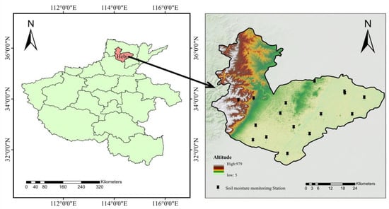
Figure 1. Location and the DEM of Hebi City.

3. Materials and Methods

3.1. Data Sets

3.1.1. Site Soil Moisture and Rainfall Data

This study collected daily soil moisture and precipitation data from 1 January 2019, to 31 December 2024, across 16 soil moisture monitoring stations. The measured soil moisture data were provided by the Agricultural Meteorological Station of the Henan Provincial Meteorological Bureau. Data acquisition was automatically performed using Time-Domain Reflectometry (TDR) sensors. These sensors established observation layers at 10 cm intervals from the soil surface, covering depths ranging from 10 to 100 cm. They simultaneously measured volumetric soil moisture and relative moisture content at each layer, with observation errors controlled within ±3%. Data collection operated continuously on an hourly basis around the clock. Given that prior studies have demonstrated soil moisture at the 20–30 cm depth is most indicative of agricultural drought [28,29], this study ultimately selected measured soil moisture data from the 10–30 cm layer at each site for subsequent analysis.

3.1.2. Sentinel Satellite Series Data

The Sentinel satellite series, a core component of the Copernicus Programme by the European Space Agency (ESA), aims to provide high-quality and high-precision remote sensing data for fields such as environmental monitoring, climate change research, and disaster management. This study primarily utilizes Sentinel-1 and Sentinel-2 satellite data, with specific product information as follows: Sentinel-1 consists of two satellites, namely Sentinel-1A and Sentinel-1B, both of which are polar-orbiting satellites. Sentinel-1A was launched on 3 April 2014, and Sentinel-1B on 25 April 2016. The mission of Sentinel-1B concluded in 2022, while Sentinel-1C was launched on 5 December 2024. Equipped with a C-band Synthetic Aperture Radar (SAR), the satellites possess all-time and all-weather observation capabilities, unaffected by cloud cover or lighting conditions. Sentinel-1 offers different resolutions depending on its imaging modes: the Strip Map (SM) mode has a resolution of 5 m × 5 m, the Interferometric Wide Swath (IW) mode 5 m × 20 m, the Extra-Wide Swath (EW) mode 20 m × 40 m, and the Wave (WV) mode 5 m × 5 m [30]. This study employs VV and VH dual-polarization Synthetic aperture radar (SAR) data from the Sentinel-1 Interferometric Wide Swath (IW) mode. With a swath width of approximately 250 km, this mode can clearly reveal soil moisture distribution at the field scale (e.g., contiguous farmland). Additionally, it features a short revisit period (6 days for a single satellite and 3 days for dual satellites), enabling high-frequency monitoring at regional scales such as county and municipal levels (e.g., weekly soil moisture change monitoring on a weekly basis). Relevant data are presented in Table 1. On the premise of ensuring the accuracy of soil moisture retrieval and drought monitoring, it balances precision and efficiency by shortening the data acquisition cycle to increase the sample size within the same period, making it the optimal mode for regional-scale studies.

Table 1. Usage of sentinel-1 data.

Data	Unit	Imaging Mode	Time Resolution	Spatial Resolution
VV	dB	IW	6 days	5 m × 20 m
VH	dB	IW	6 days	5 m × 20 m

The Sentinel-2 satellite series comprises two satellites, namely Sentinel-2A and Sentinel-2B. Sentinel-2A was launched on 23 June 2015, and Sentinel-2B on 7 March 2017. Equipped with a multispectral imager, Sentinel-2 satellites feature 13 spectral bands, covering the visible light, near-infrared, and short-wave infrared regions. These bands have ground resolutions of 10 m, 20 m, and 60 m, respectively, providing high-resolution image data that meets diverse application requirements. The Sentinel-2 data utilized in this study includes the Normalized Difference Vegetation Index (NDVI), Band B2 data, and Band B11 data. The primary reasons for selecting the above bands are as follows: First, although NDVI is not an original band of Sentinel-2, it is calculated from Band B4 (red band, 665 nm) and Band B8 (near-infrared band, 842 nm). As a core parameter characterizing vegetation coverage and growth status, its effectiveness in soil moisture retrieval and drought monitoring has been verified by numerous studies [31,32,33]. Second, Band B11 (short-wave infrared band, central wavelength of 1610 nm) is highly sensitive to the moisture content of the topsoil layer (0–5 cm). Third, Band B2 (blue band, central wavelength of 490 nm) is critical for retrieving aerosol optical depth and eliminating atmospheric scattering interference during the preprocessing stage. Although only these three types of data are selected, they roughly cover the main band ranges of Sentinel-2. Relevant data are presented in Table 2.

Table 2. Usage of sentinel-2 data.

Data	Data Definition & Source	Time Resolution	Spatial Resolution
NDVI	$NDVI={\displaystyle \frac{{\rho }_{B8}-{\rho }_{B4}}{{\rho }_{B8}-{\rho }_{B4}}}$	5 days	10 m
B2	Blue Band	5 days	10 m
B11	Shortwave Infrared Band	5 days	10 m

Currently, numerous studies have demonstrated the accuracy of high-resolution data from the Sentinel satellite series in monitoring small-scale droughts, geological hazards, and crop distribution [34,35,36]. The temporal range of the data used in this study is from 2019 to 2024, and the data were sourced from the Google Earth Engine (GEE) platform. The specific access link is: https://earthengine.google.com/.

3.1.3. ASTER GDEM Version 3.0 Elevation Data

ASTER GDEM is a global digital elevation data product jointly released by the National Aeronautics and Space Administration (NASA) and the Ministry of Economy, Trade and Industry (METI) of Japan. It is generated through calculations based on data from the Advanced Spaceborne Thermal Emission and Reflection Radiometer (ASTER), covering the land surface between 83° N and 83° S with a spatial resolution of 1 arc-second (approximately 30 m) [37]. This data features high precision and high data quality. Compared with its predecessor, ASTER GDEM v2.0, the current version offers better matching between horizontal accuracy and surface features, as well as more precise positioning. It adopts more advanced algorithms to identify and eliminate artifacts caused by clouds, shadows, and water bodies, significantly suppressing phenomena such as “ghosting” and “striping” [37,38]. Specific access link: https://www.gscloud.cn/search (accessed on 28 July 2024). Considering the influence of slope and aspect on soil moisture storage, and to fully utilize the potential role of DEM data, this study used ArcGIS 10.8 (Esri, Redlands, CA, USA) to extract slope and aspect data of the study area from the target DEM data. After undergoing uniform spatial resolution processing, these data were used as independent variables in the model.

3.1.4. GPM Global Precipitation Data

GPM global precipitation data is generated by the Global Precipitation Measurement (GPM) mission, a joint initiative of the National Aeronautics and Space Administration (NASA) and the Japan Aerospace Exploration Agency (JAXA). Primarily based on observations from the GPM Core Observatory and other low-orbit satellites, GPM data integrates multiple types of sensor data, including microwave and infrared data. Its spatial resolution is typically 0.1° × 0.1° (approximately 10 km × 10 km). For temporal resolution, multiple options are available, including 30-min, 1-h, 3-h, 1-day, and 1-month precipitation data. The GPM data used in this study spans from 2019 to 2024 and was sourced from the Google Earth Engine (GEE) platform. The specific access link is: https://earthengine.google.com/.

The extraction of GPM, DEM, and other related data requires processing multi-source remote sensing data to have consistent spatial and temporal resolutions with the Sentinel series data. First, the remote sensing data are spatially resampled to obtain data with the same spatial resolution. Second, interpolation is performed on all types of remote sensing data during time periods with no available data to achieve data with the same temporal resolution.

3.2. Methods

3.2.1. Machine Learning Models

Our preliminary research indicates that XGBoost and RF machine learning models demonstrate superior performance in multi-source remote sensing drought monitoring [21], exhibiting strong resistance to overfitting and high-dimensional data processing capabilities. This study specifically selects several commonly used ensemble learning methods to systematically validate the impact of different approaches on drought monitoring accuracy.

Random Forest (RF) is a supervised learning algorithm based on the idea of Ensemble Learning, proposed by Leo Breiman in 2001. Its core lies in constructing multiple Decision Trees and performing ensemble voting (for classification tasks) or averaging (for regression tasks) on the results. This approach reduces the overfitting risk of a single Decision Tree while improving the model’s generalization ability and stability. As a typical implementation of the Bagging (Bootstrap Aggregating) ensemble framework, Random Forest retains the advantages of Decision Trees-such as “strong interpretability and insensitivity to data distribution”. Furthermore, by introducing two key randomness mechanisms, “random sample sampling” and “random feature selection”, it effectively addresses the critical issues of a single Decision Tree, including vulnerability to noisy data and high model variance. It is widely applied in machine learning tasks such as classification, regression, and feature importance evaluation. The following are the parameters of the RF model in Scikit-learn and their core functions. as shown in Table 3.

Table 3. Random Forest Parameters and Core Functions.

Parameter Name	Core Functions
n_estimators	Control the number of decision trees in a random forest
max_depth	Maximum depth limit per decision tree
max_features	Maximum features for node splitting in a single decision tree
min_samples_split	Minimum samples required to split an internal node in a decision tree
min_samples_leaf	Minimum samples required for a leaf node in a decision tree
random_state	Random seed for random forest control

XGBoost (extreme Gradient Boosting), proposed by Tianqi Chen, is an optimized implementation of the Gradient Boosting Decision Tree (GBDT). By integrating weak learners (CART trees) and introducing regularization as well as efficient optimization strategies, it exhibits excellent generalization ability and training efficiency in classification, regression, and ranking tasks, and is widely applied in machine learning competitions and industrial scenarios. Its core idea is to iteratively construct new decision trees along the gradient descent direction based on the prediction residuals of the previous round of the ensemble model. Finally, the prediction results of all trees are weighted and summed to obtain the final output. The following are the parameters and their core functions of the XGBoost model in XGBClassifier. as shown in Table 4.

Table 4. XGBoost Parameters and Core Functions.

Parameter Name	Core Functions
n_estimators	Control number of trees to balance fitting ability and computational cost
learning_rate	Scale individual tree weights to adjust model convergence speed and stability
max_depth	Limit individual tree depth to control model complexity and prevent overfitting
subsample	Row sampling ratio to introduce randomness and reduce overfitting risk
colsample_bytree	Column sampling ratio to reduce feature redundancy impact and improve ensemble diversity
reg_alpha	L1 regularization to enable feature selection and weight sparsification
reg_lambda	L2 regularization to shrink weights and prevent excessive influence of single features
objective	Define loss function to adapt to classification task types (binary/multi-class)
random_state	Fix random processes to ensure result reproducibility

RF-RFE (Random Forest-Recursive Feature Elimination), a feature selection method that combines Random Forest (RF)-based feature importance evaluation with Recursive Feature Elimination (RFE)-based iterative screening. This algorithm uses RF to quantify the contribution of features to the model’s predictive performance, then adopts a recursive strategy of “gradually eliminating the least important features + retraining the model for validation” to screen out the optimal feature subset. RF-RFE (Random Forest-Recursive Feature Elimination), a feature selection method that combines Random Forest (RF)-based feature importance evaluation with Recursive Feature Elimination (RFE)-based iterative screening. This algorithm uses RF to quantify the contribution of features to the model’s predictive performance, then adopts a recursive strategy of “gradually eliminating the least important features + retraining the model for validation” to screen out the optimal feature subset. The following are the core parameters newly added by RFE (taking sklearn.feature_selection.RFE as an example) and their functions.as shown in Table 5.

Table 5. RFE Parameters and Core Functions.

Parameter Name	Core Functions
estimator	Specified base model
n_features_to_select	Final number of features retained
step	Number of features removed per iteration
verbose	Level of detail in iteration output

3.2.2. Sample Collection and Processing

The main crop grown in the study area is wheat, and soil water content is one of the key factors affecting wheat growth. There are significant differences in the impact of soil water content at different depths on wheat growth, which is closely related to the root distribution characteristics of wheat and the water demand law during its growth period. Studies have shown [39] that during the critical growth period of wheat (from jointing to booting stage), wheat roots have penetrated deeply into the middle soil layer, and the water demand accounts for more than 50% of the total water demand throughout the growth period. Therefore, soil water content at a depth of 20 cm was selected as the reference data to reflect the status of agricultural drought, as shown in Table 6.

Table 6. Drought classification of relative soil moisture.

Grade	Type	Relative Soil Moisture at Depth of 20 cm
1	No drought	60% < RSM
2	Mild drought	50% < RSM ≤ 60%
3	Moderate drought	40% < RSM ≤ 50%
4	Severe drought	30% < RSM ≤ 40%
5	Extreme drought	RSM ≤ 30%

Due to the complexity of the formation mechanism of agricultural drought, constructing a more comprehensive drought monitoring system often requires integrating multi-source data (e.g., meteorological, remote sensing, and soil observation data). However, there are significant differences in spatial and temporal resolutions among data from different sources. If such heterogeneous-resolution data are directly input into the model, it will result in poor spatiotemporal matching of data and disordered dimensionality of model input features, thereby reducing the accuracy of drought monitoring and the reliability of results. Therefore, it is necessary to perform resampling preprocessing on the original data. Focusing on drought monitoring in small-scale areas, this study attempts to take high-resolution remote sensing data as the benchmark and uniformly resample all data sources to a spatial resolution of 20 m and a temporal resolution of 2 × 5 days, consistent with Sentinel-2 data. This lays a data foundation for the subsequent construction of a high-precision drought monitoring model.

3.2.3. Model Construction

Main Steps: 1. Automatic soil moisture monitoring stations in Hebi City were selected as soil moisture sampling points for this study. Other data under the same coordinates were collected and classified into different drought factors according to their data types. 2. Initial models were constructed based on three machine learning algorithms. On the basis of incorporating all drought factors, controlled experiments involving the removal of a single factor one by one were conducted. Combined with the correlation coefficient (R) and Relative Root Mean Square Error (RRMSE), the model’s response degree to each factor was quantified, and the contribution weight of different drought factors was evaluated. 3. Models were constructed by sequentially accumulating the number of samples starting from 2019, with the actual drought data of 2023 used as the true values of the model test set. The influence of the number of research samples on the performance of different models was analyzed. 4. The optimal combination of drought factors was selected based on the sensitivity analysis results. The optimal training sample size was determined by combining sample size evaluation, and a high-precision drought monitoring model was reconstructed. Based on the model output, the agricultural drought grades in the study area of Hebi City were calculated. 5. The calculated drought grades were used to display the spatial distribution of agricultural drought in Hebi City. The flow chart of the study is shown in Figure 2.

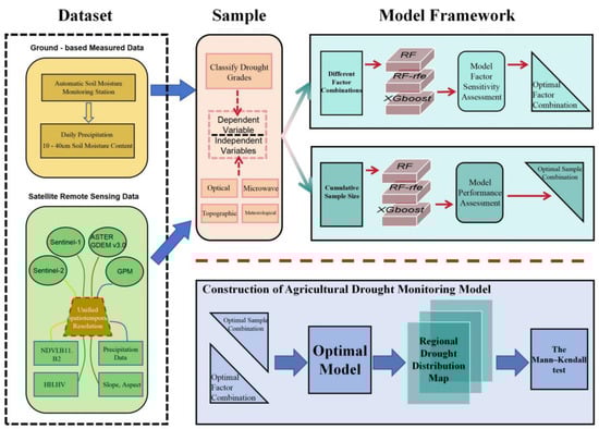
Figure 2. Research Flow Chart.

3.3. Model Accuracy Evaluation

3.3.1. Model Factor Sensitivity Assessment

This study considers the differences in the response of agricultural drought to different variable combinations, comprehensively evaluates the reliability and robustness of agricultural drought variable combinations, and selects two commonly used statistical evaluation indicators to assess the models of different factor combinations under the three machine learning algorithms. The calculation formulas of the two indicators are shown below. Relative Root Mean Square Error (RRMSE) and Pearson Correlation Coefficient (R).

$$RRMSE={\displaystyle \frac{\sqrt{\frac{\sum _{i=1}^N{\left(Y-X\right)}^2}{N}}N}{\sum _{i=1}^N{Y}_i}}$$

(1)

$$R={\displaystyle \frac{{\sum }_{i=1}^N\left(X_i-{\mu }_X\right)\left(Y_i-{\mu }_Y\right)}{\left(N-1\right){\delta }_X{\delta }_Y}}$$

(2)

In the formula, X represents the monitored value of drought grade, Y represents the actual value of drought grade. In Formula (2), ${\mu }_X$ denotes the average value of the monitored values, ${\mu }_Y$ denotes the average value of the actual values, ${\delta }_X$ and ${\delta }_Y$ represent the standard deviations of the monitored values and the actual values, respectively.

3.3.2. Model Performance Evaluation

Based on the selected optimal variable combination for drought monitoring and the optimal training sample size, three machine learning classification models will be constructed through experiments. Below, the performance of each machine learning classification model will be evaluated in detail using four key metrics: precision, accuracy, F1-score (harmonic mean), and recall. The specific calculation formulas are shown below.

$$accuracy={\displaystyle \frac{TP+TN}{TP+FN+FP+TN}}$$

(3)

$$precision={\displaystyle \frac{TP}{TP+FP}}$$

(4)

$$recall={\displaystyle \frac{TP}{TP+FN}}$$

(5)

$$f1-score={\displaystyle \frac{2\ast recall\ast precision}{recall+precision}}$$

(6)

In the formulas: TP (True Positive): The number of samples where the model classifies the category as A, and the actual category of the samples is also A.FP (False Positive): The number of samples where the model classifies the category as A, but the actual category of the samples is not A.FN (False Negative): The number of samples where the actual category of the samples is A, but the model classifies the category as not A.TN (True Negative): The number of samples where the actual category of the samples is not A, and the model also classifies the category as not A. Meanwhile, attention should be paid to distinguishing between precision and accuracy. Accuracy refers to the proportion of correctly classified samples by the model to the total number of samples, while precision refers to the proportion of samples that are actually positive among the samples classified as positive by the model.

Since precision, recall, and F1-score can only evaluate the model’s ability to identify drought of the same grade, and in actual drought scenarios, the number of samples across different drought grades often shows an uneven distribution. This makes such metrics unable to intuitively reflect the comprehensive performance of the drought monitoring model. To address this, the experiment will weight the above three metrics based on the number of samples of different drought grades in actual scenarios, thereby evaluating the model performance in a manner more aligned with practical application needs.

3.3.3. Timing Sequence Analysis Method

The Mann–Kendall test is suitable for analyzing the long-term trends and abrupt change characteristics of multi-source remote sensing data. It exhibits strong robustness to a small number of outliers and can effectively reveal the trend evolution patterns and abrupt change points of the entire time series. Based on the above advantages, this method has been widely applied in studies related to agricultural drought change trends, providing important technical support and reference for the time series analysis of agricultural drought.

For the time series variable sequence x₁, x₂, …, x_n, where n is the length of the time series, when n > 10:

$$Z=\{\begin{array}{c}{\displaystyle \frac{s-1}{\sqrt{Var\left(S\right)}}},S>0\\ 0,fS=0\\ {\displaystyle \frac{s+1}{\sqrt{Var\left(S\right)}}},S<0\end{array}$$

(7)

$$U_{Bk}={\displaystyle \frac{S_k-E\left(S\right)}{\sqrt{Var\left(S\right)}}},k=\mathrm{1,2},\dots ,n$$

(8)

$$\{\begin{array}{c}{U}_{Bk}=-U_{Fk}\\ k^{\prime }=n+1-k\end{array}$$

(9)

Given a significance level of 0.05, where $U_{Fk}$ represents the standard normal distribution and $U_{Bk}$ denotes the inverse sequence of $U_{Fk}$. If the curves $U_{Bk}$ and $U_{Fk}$ intersect, it indicates a sudden change starting at that point. If Z > 0, the time series exhibits an upward trend; conversely, a negative value indicates a downward trend. When |Z| > 1.96, a 95% confidence level is achieved.

4. Results

4.1. Selection of Model Sample Types

Two indicators, RRMSE and R, shown in Figure 3, reflect the contribution of different variable combinations to various models. According to the results, under the variable conditions of without Microwave, without Precipitation, and full factors, the XGBoost model exhibits the smallest RRMSE error and better linear fitting ability compared with the other two models. The RF model outperforms the XGBoost model in these two indicators under the conditions of without DEM and without Optical. When all factors are input, the XGBoost model achieves the minimum RRMSE of 0.45 and strong linear fitting ability, indicating that it is more efficient in fusing and utilizing multiple factors. In contrast, the RF-RFE model has a higher error than the basic RF model, but its linear correlation is not weaker than that of the RF model. This may be due to the loss of key information, resulting in the outcome that “excessive simplification of features reduces accuracy”, which may also be related to algorithm adaptability.

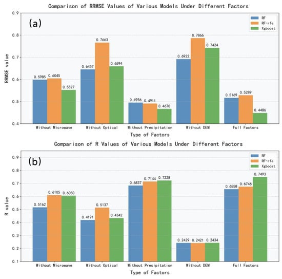
Figure 3. Performance metrics of the three models under different sample combinations: (a) RRMSE; (b) R.

After comparing the scenarios with missing factors, it can be found that removing “DEM” leads to a significant increase in the RRMSE of the three models, and the correlation coefficient R drops to around 0.2. This indicates that DEM plays the role of a “core discriminant factor” among the four types of factors; its absence makes it difficult for the models to capture key patterns, resulting in inaccurate predictions. When “Precipitation” is removed, the R values of RF-based models are the highest—even higher than those under the full-factor scenario—and the R value of the XGBoost model also reaches 0.72. This finding is corroborated by the RRMSE values, suggesting that the Precipitation Type factor contributes little to the models and may even introduce noise, making it a potential redundant factor. However, analyzing the results alone, the differences in R between the RF-based models (with “Precipitation” removed) and the full-factor scenario are only 0.04, and the differences in RRMSE are as small as 0.02. Additionally, under the full-factor condition, the XGBoost model achieves the optimal RRMSE and R values. Therefore, the full-factor combination is still determined as the optimal variable combination through comprehensive evaluation. Subsequent discussions can be based on these results, integrating the observation characteristics and physical significance of precipitation data to explore the reasons for the low contribution of the “Precipitation Type” factor and optimize the rationality of selecting precipitation-related factors.

4.2. Cumulative Selection of Model Samples

In this experiment, the measured drought grades of 2023 were used as the test set, and the total number of samples was expanded by accumulating data from 2019 to 2024 (excluding 2023). Under the full-factor condition, three machine learning methods were used sequentially to construct models, and finally, the trend chart of model performance changing with the cumulative number of samples (shown in Figure 4) was obtained.

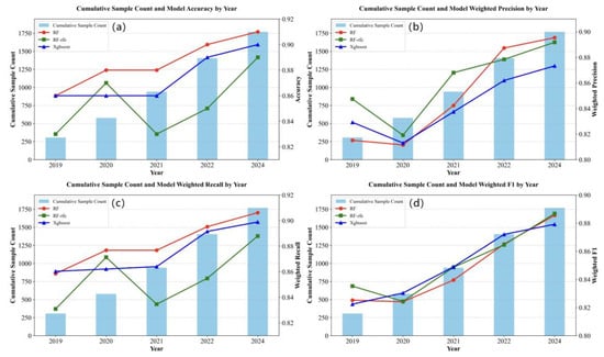
Figure 4. Performance metrics of the three models with cumulative sample size: (a) Accuracy; (b) Precision; (c) Recall; (d) F1-score.

As shown in Figure 4, the performance of the three models generally fluctuates first and then increases continuously with the increase in the number of samples. In the early stage, when the sample size was small (the basic samples in 2019 were limited), the models were prone to overfitting or underfitting. As the sample size expanded (the sample size increased sharply after 2022), the models learned more comprehensive patterns, leading to improved generalization ability. RF-RFE showed the largest fluctuations in the early stage (2020–2021). Due to feature simplification, RF-RFE was more sensitive to small-sample fluctuations. However, as the number of samples increased, when the cumulative sample period exceeded three years, the performance improvement rate of RF-RFE was significantly faster than that of the RF and XGBoost models, indicating considerable potential. Limited by the latest update timeliness of data, future studies can attempt to further increase the sample size.

4.3. Optimal Model Performance

The training set and test set in this study contained 1756 samples and 440 samples, respectively. The models used were Random Forest (RF), Random Forest based on Recursive Feature Elimination (RF-RFE), and Extreme Gradient Boosting (XGBoost). Box plots were generated based on the results of ten training runs.

As can be seen from the box plots in Figure 5, the medians of test set accuracy for the three models are 89%, 87%, and 89%, respectively. Accuracy reflects the “overall proportion of correct predictions”. XGBoost and RF outperform RF-RFE in this metric; additionally, XGBoost shows a more concentrated distribution, indicating better model stability than RF and superior comprehensive discriminative ability for samples. The accuracy of RF-RFE decreases significantly, which is presumably due to excessive simplification of the model structure during feature selection, resulting in the loss of key discriminative information. When analyzing other metrics (Figure 3), including Weighted Precision, Weighted Recall, and Weighted F1-Score, RF-RFE slightly outperforms RF only in terms of Weighted F1-Score. For all other metrics, the performance follows the order: XGBoost > RF > RF-RFE. Although RF-RFE marginally surpasses RF in Weighted F1-Score, its overall performance remains lower. Combined with other metrics, this slight advantage is more likely attributed to “simplified model structure after feature reduction, which reduces both misjudgments and missed judgments simultaneously but with a limited reduction range” rather than a genuine improvement in model performance.

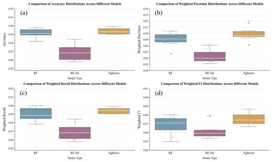
Figure 5. Performance Comparison of Various Models: (a) Accuracy; (b) Precision; (c) Recall; (d) F1 Score.

4.4. Drought Monitoring Results

In summary, under the conditions of full-factor input and sufficient data support, the drought monitoring model constructed using XGBoost achieves the optimal performance. However, the other two models still hold value: the median accuracy of RF reaches 89%, and RF-RFE can also provide references for feature-simplified modeling. This study selected a drought event that occurred in Hebi City in October 2023. The results of the three models are basically consistent with the simultaneous rainfall and soil moisture briefing released by the Henan Provincial Department of Water Resources (from 8:00 on 1 October to 8:00 on 1 November: the surface soil in northern Henan, western Henan, and parts of southern Henan suffered from moisture deficiency, with local mild drought). The specific drought distribution is as follows.

Figure 6, Figure 7 and Figure 8 clearly illustrate the dynamic process of a complete drought event in the study area during the autumn of 2023. This event occurred from 5 September to 25 November, and the drought conditions exhibited significant phased changes and fluctuation characteristics. The drought monitoring results based on the three models show a high degree of consistency, with the specific evolution of the drought and its impacts on winter wheat growth as follows:

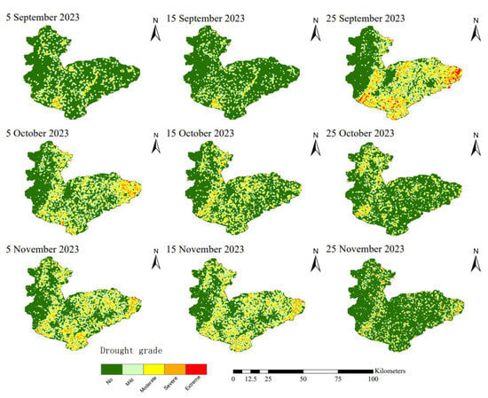
Figure 6. Drought Distribution Map of Hebi City Based on Random Forest Model.

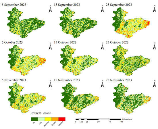
Figure 7. Drought Distribution Map of Hebi City Based on Random Forest—Recursive Feature Elimination Model.

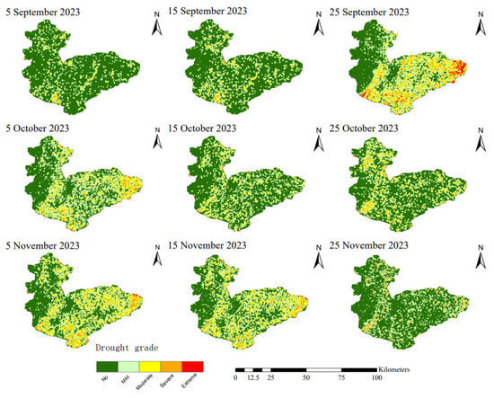
Figure 8. Drought Distribution Maps for Hebi City Based on Xgboost Models.

Before 15 September, the study area received continuous rainfall for multiple days, which effectively replenished soil moisture. No obvious drought occurred in most areas of Hebi City, and the soil moisture met the basic needs of agricultural production. After 15 September, drought signs first appeared in the eastern and southwestern parts of the region, and the drought severity escalated rapidly. It reached its peak on 25 September—areas affected by moderate and severe drought covered most of eastern Hebi City and parts of southern Hebi City, posing a significant threat to agricultural production. This period coincided with the critical stage of winter wheat sowing and emergence in Hebi City. Insufficient soil moisture prevented wheat seeds from absorbing an adequate amount of water required for germination in a timely manner. This not only significantly prolonged the time for radicles and plumules to break through the seed coat but also notably reduced the emergence rate, exerting an adverse impact on the early-stage population establishment of winter wheat.

On 25 October, the drought condition was partially alleviated: only scattered moderate drought areas remained in the region, the drought severity in most areas decreased to mild drought or below, and soil moisture improved accordingly. However, by 5 November, the drought intensified again. Compared with the drought peak on 25 September, the coverage of severe and moderate drought was significantly reduced, and the impact was lessened. By 25 November, this drought event basically ended: most areas of Hebi City returned to a non-drought state, and the remaining moderate drought areas were also scattered. At this time, winter wheat in the study area was mainly at the seedling stage, with some areas having entered the tillering stage. This growth stage directly determines wheat’s cold resistance during overwintering and its regreening growth trend in the following year. Therefore, the effective alleviation of drought is of great significance for ensuring the stable growth of winter wheat.

Overall, the drought evolution trends monitored by the three models are basically consistent, all experiencing a complete process: The evolution of this drought event can be divided into five distinct phases: The initial phase showed no drought to mild drought conditions. During the middle phase, drought intensity steadily increased and reached its peak. Subsequently, the drought experienced a period of temporary relief. In the later phase, drought conditions briefly intensified again. By the end of the study period, the drought had completely subsided. The consistency of the monitoring results provides a reliable basis for the analysis of drought events.

When comparing the spatial distribution maps generated by the three machine learning models, the XGBoost model demonstrates the optimal fitting effect based on the previous model performance evaluation results. Compared with the XGBoost model, the RF-RFE model shows significantly higher sensitivity to drought: its probability of identifying drought conditions at each time node is 5.45% higher on average, with the identification probability for moderate and severe drought grades being 2.3% higher. In contrast, the RF model without feature selection has an average drought identification probability that is 0.92% lower. Moreover, the differences between the RF model and the XGBoost model in moderate and severe drought grades are minimal and negligible. Taking the most severe drought stage on 25 September as an example, the XGBoost and RF models indicate that 17.3% and 15.4% of the area, respectively, experienced drought of varying degrees, while the identification proportion of the RF-RFE model was as high as 26.6%.

The possible reasons for this are as follows: After Recursive Feature Elimination (RFE), the RF-RFE model retains key features that are more sensitive to drought responses (such as soil moisture content and vegetation coverage), reducing interference from irrelevant features. This lowers the model’s threshold for capturing drought signals, leading to an overestimation of the drought range. In contrast, the RF model does not undergo feature optimization, and redundant features may weaken its ability to extract drought information, resulting in a slightly lower identification probability than XGBoost. XGBoost, however, balances feature weights and model complexity through a gradient boosting mechanism. It not only avoids the over-sensitivity of RF-RFE but also reduces the information loss of RF, ultimately achieving a more optimal fitting effect.

5. Discussion

When agricultural drought occurs in irrigable farmland, farmers often alleviate it through irrigation. Therefore, whether drought has occurred in farmland can be inferred inversely based on irrigation activities in the farmland. This study identifies irrigation signals based on whether precipitation during periods of increasing soil moisture exceeds 5 mm. When the increase in soil moisture exceeds 0.04 cm³/cm³ and concurrent precipitation remains below 5 mm, the rise in soil moisture during that period is attributed to irrigation; otherwise, it is attributed to precipitation events. Similar technical approaches have been employed in previous studies [40,41]. has shown that during drought periods, daily precipitation of less than 5 mm may not be considered effective precipitation, as it has no significant impact on soil moisture content at a depth of 20 cm. Taking Figure 9 as an example, an automatic soil moisture monitoring station in Hebi City (2023) showed three obvious irrigation signals: under the condition of precipitation below the 5 mm threshold, the soil moisture content increased suddenly and remained at a high level for a relatively long time. Among these signals, the third one corresponded in time to a drought event that occurred in Hebi City during the autumn of 2023. This irrigation signal further confirms the severity of this drought event.

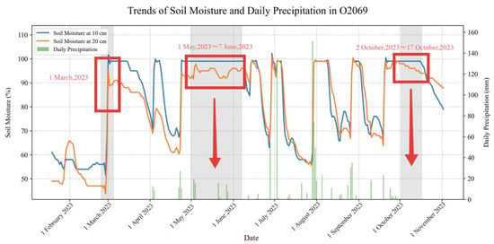
Figure 9. Variation Trends in Soil Moisture Content and Precipitation at Site O2069.

To investigate the practical application value of drought monitoring model results and accurately capture the critical time points of abrupt transitions from non-drought to drought conditions, this study examines the drought process in Hebi City during the autumn of 2023. Focusing on the time interval from 5 August 2023, to 25 December 2023, it systematically explores the temporal evolution patterns of the drought monitoring model. The data employed in this study comprised simulated outputs from three target drought monitoring models. Data preprocessing centered on the core indicator “proportion of area affected by drought events”: based on the spatial scope of the study area, the proportion of the region’s total area experiencing drought at a given time point was calculated to quantify the severity of drought at that moment. The temporal resolution of the data was uniformly set to 3 days to ensure consistency in the time scale for the time-series analysis. Based on this, the Mann–Kendall test was employed to conduct time-series analysis on the “drought area proportion time-series data” output by the three monitoring models. This ultimately characterized the continuous change trends of agricultural drought during the study period, providing a basis for the dynamic monitoring of drought processes (Figure 10, Figure 11 and Figure 12).

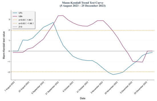
Figure 10. Mann–Kendall test based on the RF model.

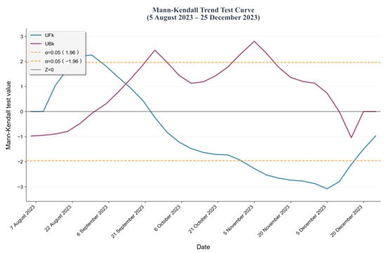
Figure 11. Mann–Kendall test based on the RF-rfe model.

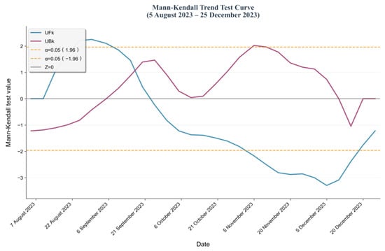
Figure 12. Mann–Kendall test based on the Xgboost model.

A significance level of 0.05 was set for this test, which implements the analysis by calculating two key statistics: the first is the forward-order statistic $U_{Fk}$, and the second is the backward-order statistic $U_{Bk}$ (obtained by reversing the time series of $U_{Fk}$), both of which follow a standard normal distribution; in terms of mutation determination, if there is an intersection between the two statistic curves of $U_{Fk}$ and $U_{Bk}$, the time node corresponding to this intersection indicates the moment when a mutation occurs in the drought series; for trend judgment, it is necessary to introduce the core statistic Z of the MK test—if Z > 0, it means the drought time series shows an overall upward trend during the study period, while if Z < 0, it shows a downward trend; regarding the confidence test, based on the characteristics of the standard normal distribution, when the absolute value of the statistic |Z| > 1.96, the trend change of the drought series can be considered to have passed the 95% confidence test, i.e., the trend result is statistically significant; as shown in Figure 8 and Figure 9, overall, in the three Mann–Kendall tests, the statistic curves of $U_{Fk}$ and $U_{Bk}$ all intersect around 18 September, which is consistent with the occurrence time of the drought, and in some periods, the $U_{Fk}$ or $U_{Bk}$ statistic exceeds the critical value range corresponding to α = 0.05, reflecting that the trend evolution during this period has strong statistical regularity; by comparing the three test results, the drought process depicted by the RF model is more complete—its two mutation points are highly consistent with the occurrence and end times of the drought, and at the same time, the RF model shows a more significant performance of exceeding the α = 0.05 curve with a relatively more prominent change trend; thus, in terms of drought process characterization and trend significance, RF is relatively superior to XGBoost.

In this study, there is a significant correlation between model performance and data selection. Due to space limitations, only some of the issues identified during the research process are discussed here. First, in the experiment on the selection of model sample types, it was observed that after removing the “Precipitation” factor, some models showed better performance in terms of RRMSE (Relative Root Mean Square Error) and R (Coefficient of Determination) than when all factors were included. Possible reasons for this phenomenon include the following: the resolution of the selected GPM (Global Precipitation Measurement) data is significantly lower than that of other input data. Even if resampling technology is used to adjust its spatial/temporal resolution, it is still difficult to completely eliminate data information loss caused by resolution mismatch. Additionally, the GPM data itself may have observation biases or data gaps in local time periods. When inputted collaboratively with high-resolution data, such differences in data quality may interfere with the model’s accurate learning of the correlations between factors, which in turn leads to a decline in the model’s fitting effect when all factors are inputted. Meanwhile, by comparing the drought distribution map with the DEM map (see Figure 13), it was found that the probability of drought occurrence in the western mountainous areas of the study region is significantly lower.

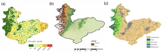
Figure 13. (a) Arid Distribution Map, and (b) Digital Elevation Map of the Study Area, (c) Land Use Map of the Study Area.

Two possible explanations are inferred as follows: First, after DEM data is input into the model, the impacts of plain and mountainous terrain on processes such as water movement and evapotranspiration differ, leading to variations in the model’s drought identification results across different topographic regions. This has been investigated in greater depth by Hawthorne S et al. [42] and Oberski T et al. [43] Second, mountainous areas are dominated by forestlands. Forest canopies have a strong capacity to intercept precipitation, and litter layers and soils under forests exhibit high abilities to store water, resulting in better water retention. This, in turn, reduces the probability of drought occurrence—a view also supported in the study by Calder, I. R [44].

6. Conclusions

This study takes Hebi City as the research area, integrates Sentinel series remote sensing data and other multi-source data, and constructs a medium-high resolution agricultural drought monitoring model. Three machine learning models—Random Forest (RF), Random Forest based on Recursive Feature Elimination (RF-RFE), and Extreme Gradient Boosting (XGBoost)—were selected to conduct optimal variable combination screening, sample size adaptation, and model performance analysis. Additionally, drought distribution maps were drawn to screen out the agricultural drought monitoring model suitable for the research area. The main conclusions are as follows:

• Sentinel series remote sensing data with medium resolution performed well in the three models, and the accuracy of drought identification exceeded 86% in all cases.
• Among all input factors, Digital Elevation Model (DEM) data had the greatest influence and was a core identification factor. Removing this factor would lead to a sharp increase in the Relative Root Mean Square Error (RRMSE).
• Compared with the other two models, XGBoost was superior to the other RF-based models in terms of accuracy and stability; under the same sample conditions, RF-RFE was the most sensitive to drought responses.
• The drought monitoring model developed in this study can provide reference for irrigation scheduling in the study area by identifying drought occurrence characteristics. Surface land use types—particularly vegetation cover—influence regional water budgets and drought formation processes, potentially affecting monitoring accuracy. Future work may consider incorporating these factors into model optimization to further enhance the precision of irrigation guidance.

References

- Mishra, A.K.; Singh, V.P. A review of drought concepts. J. Hydrol. 2010, 391, 202–216. [Google Scholar] [CrossRef]
- Sánchez, N.; González-Zamora, Á.; Martínez-Fernández, J.; Piles, M.; Pablos, M. Integrated remote sensing approach to global agricultural drought monitoring. Agric. For. Meteorol. 2018, 259, 141–153. [Google Scholar] [CrossRef]
- Zhou, H.; zhi Zhao, W. Modeling soil water balance and irrigation strategies in a flood-irrigated wheat-maize rotation system. A case in dry climate, China. Agric. Water Manag. 2019, 221, 286–302. [Google Scholar] [CrossRef]
- Mathobo, R.; Marais, D.; Steyn, J.M. Calibration and validation of the SWB model for dry beans (Phaseolus vulgaris L.) at different drought stress levels. Agric. Water Manag. 2018, 202, 113–121. [Google Scholar] [CrossRef]
- Paciolla, N.; Corbari, C.; Mancini, M. Time continuous two-source energy-water balance modelling of heterogeneous crops: FEST-2-EWB. J. Hydrol. 2023, 619, 129265. [Google Scholar] [CrossRef]
- Cai, G.; Carminati, A.; Gleason, S.M.; Javaux, M.; Ahmed, M.A. Soil-plant hydraulics explain stomatal efficiency-safety tradeoff. Plant Cell Environ. 2023, 46, 3120–3127. [Google Scholar] [CrossRef] [PubMed]
- Wankmüller, F.J.; Delval, L.; Lehmann, P.; Baur, M.J.; Cecere, A.; Wolf, S.; Or, D.; Javaux, M.; Carminati, A. Global influence of soil texture on ecosystem water limitation. Nature 2024, 635, 631–638. [Google Scholar] [CrossRef]
- Wang, J.; Chang, L.; Aggarwal, S.; Abari, O.; Keshav, S. Soil moisture sensing with commodity RFID systems. In Proceedings of the 18th International Conference on Mobile Systems, Applications, and Services, Toronto, ON, Canada, 15–19 June 2020; pp. 273–285. [Google Scholar]
- Matilla, D.M.; Murciego, A.L.; Jiménez-Bravo, D.M.; Mendes, A.S.; Leithardt, V.R. Low-cost Edge Computing devices and novel user interfaces for monitoring pivot irrigation systems based on Internet of Things and LoRaWAN technologies. Biosyst. Eng. 2022, 223, 14–29. [Google Scholar] [CrossRef]
- Luo, K.; Chen, Y.; Lin, R.; Liang, C.; Zhang, Q. A Portable Agriculture Environmental Sensor with a Photovoltaic Power Supply and Dynamic Active Sleep Scheme. Electronics 2024, 13, 2606. [Google Scholar] [CrossRef]
- Cai, J.; Zhao, W.; Ding, T.; Yin, G. Generation of High-Resolution Surface Soil Moisture over Mountain Areas by Spatially Downscaling Remote Sensing Products Based on Land Surface Temperature–Vegetation Index Feature Space. J. Remote Sens. 2025, 5, 0437. [Google Scholar] [CrossRef]
- Thenkabail, P.S. Remote Sensing Handbook, Volume VI: Droughts, Disasters, Pollution, and Urban Mapping; CRC Press: Boca Raton, FL, USA, 2024. [Google Scholar]
- Ghasempour, F.; Yamaç, S.S.; Sekertekin, A.; Iban, M.C.; Kutoglu, S.H. Spatiotemporal Agricultural Drought Assessment and Mapping Its Vulnerability in a Semi-Arid Region Exhibiting Aridification Trends. Agriculture 2025, 15, 2060. [Google Scholar] [CrossRef]
- Zhu, L.; Tian, G.; Wu, H.; Ding, M.; Zhu, A.-X.; Ma, T. Regional assessment of soil moisture active passive enhanced L3 Soil Moisture Product and Its Application in Agriculture. Remote Sens. 2024, 16, 1225. [Google Scholar] [CrossRef]
- Zou, L.; Cao, S.; Sanchez-Azofeifa, A. Evaluating the utility of various drought indices to monitor meteorological drought in Tropical Dry Forests. Int. J. Biometeorol. 2020, 64, 701–711. [Google Scholar] [CrossRef] [PubMed]
- Wang, L.; Guo, N.; Yue, P.; Hu, D.; Sha, S.; Wang, X. Regulation of evapotranspiration in different precipitation zones and its application in high-temperature and drought monitoring. Remote Sens. 2022, 14, 6190. [Google Scholar] [CrossRef]
- Yang, S.; Zhang, D.; Sun, L.; Wang, Y.; Gao, Y. Assessing drought conditions in cloudy regions using reconstructed land surface temperature. J. Meteorol. Res. 2020, 34, 264–279. [Google Scholar] [CrossRef]
- Mullapudi, A.; Vibhute, A.D.; Mali, S.; Patil, C.H. A review of agricultural drought assessment with remote sensing data: Methods, issues, challenges and opportunities. Appl. Geomat. 2023, 15, 1–13. [Google Scholar] [CrossRef]
- Li, Y.; Dong, Y.; Yin, D.; Liu, D.; Wang, P.; Huang, J.; Liu, Z.; Wang, H. Evaluation of drought monitoring effect of winter wheat in Henan province of China based on multi-source data. Sustainability 2020, 12, 2801. [Google Scholar] [CrossRef]
- Prudente, V.H.R.; Martins, V.S.; Vieira, D.C.; e Silva, N.R.d.F.; Adami, M.; Sanches, I.D.A. Limitations of cloud cover for optical remote sensing of agricultural areas across South America. Remote Sens. Appl. Soc. Environ. 2020, 20, 100414. [Google Scholar] [CrossRef]
- Tian, G.; Zhu, L. Drought monitoring of winter wheat in Henan province, China based on multi-source remote sensing data. Agronomy 2024, 14, 758. [Google Scholar] [CrossRef]
- Kercheva, M.; Ganeva, D.; Dimitrov, Z.; Atanasov, A.Z.; Kuncheva, G.; Kolchakov, V.; Nikolova, P.; Dimitrov, S.; Nenov, M.; Filchev, L. Integrating Remote Sensing and Ground Data to Assess the Effects of Subsoiling on Drought Stress in Maize and Sunflower Grown on Haplic Chernozem. Agriculture 2025, 15, 1644. [Google Scholar] [CrossRef]
- Abbes, A.B.; Jarray, N.; Farah, I.R. Advances in remote sensing based soil moisture retrieval: Applications, techniques, scales and challenges for combining machine learning and physical models. Artif. Intell. Rev. 2024, 57, 224. [Google Scholar] [CrossRef]
- Wang, F.; Yu, C.; Xiong, L.; Chang, Y. How can agricultural water use efficiency be promoted in China? A spatial-temporal analysis. Resour. Conserv. Recycl. 2019, 145, 411–418. [Google Scholar] [CrossRef]
- Manago, N.; Hongo, C.; Sofue, Y.; Sigit, G.; Utoyo, B. Transplanting date estimation using sentinel-1 satellite data for paddy rice damage assessment in Indonesia. Agriculture 2020, 10, 625. [Google Scholar] [CrossRef]
- Liu, W.; Ma, S.; Feng, K.; Gong, Y.; Liang, L.; Tsubo, M. The suitability assessment of agricultural drought monitoring indices: A case study in inland river basin. Agronomy 2023, 13, 469. [Google Scholar] [CrossRef]
- Rusdi, M.; Budi, M.; Farhan, A. agricultural droughts monitoring of aceh besar regency rice production center, Aceh, Indonesia–application vegetation conditions index using Sentinel-2 image data. J. Ecol. Eng. 2023, 24, 159–171. [Google Scholar]
- Ghavamsaeidi Noghabi, S.; Yaghoobzadeh, M.; Najafi Mood, M.H. The Evaluation of Climate Change Impact on Agricultural Drought by Soil Moisture Deficit Index Using Fifth Report Models and Scenarios. Iran. J. Soil Water Res. 2020, 50, 2425–2438. [Google Scholar]
- Alahmad, T.; Neményi, M.; Nyéki, A. Soil Moisture Content Prediction Using Gradient Boosting Regressor (GBR) Model: Soil-Specific Modeling with Five Depths. Appl. Sci. 2025, 15, 5889. [Google Scholar] [CrossRef]
- Torres, R.; Snoeij, P.; Geudtner, D.; Bibby, D.; Davidson, M.; Attema, E.; Potin, P.; Rommen, B.; Floury, N.; Brown, M. GMES Sentinel-1 mission. Remote Sens. Environ. 2012, 120, 9–24. [Google Scholar] [CrossRef]
- Varghese, D.; Radulović, M.; Stojković, S.; Crnojević, V. Reviewing the potential of Sentinel-2 in assessing the drought. Remote Sens. 2021, 13, 3355. [Google Scholar] [CrossRef]
- Wu, S.-Y.; Bao, Y.-S.; Li, Y.-F.; Wu, Y. Joint retrieval of soil moisture from Sentinel-1 and Sentinel-2 remote sensing data based on neural network algorithm. Trans. Atmos. Sci. 2021, 44, 636–644. [Google Scholar]
- Son, M.-B.; Chung, J.-H.; Lee, Y.-G.; Kim, S.-J. A comparative analysis of vegetation and agricultural monitoring of Terra MODIS and Sentinel-2 NDVIs. J. Korean Soc. Agric. Eng. 2021, 63, 101–115. [Google Scholar]
- Schellenberg, K.; Jagdhuber, T.; Zehner, M.; Hese, S.; Urban, M.; Urbazaev, M.; Hartmann, H.; Schmullius, C.; Dubois, C. Potential of Sentinel-1 SAR to assess damage in drought-affected temperate deciduous broadleaf forests. Remote Sens. 2023, 15, 1004. [Google Scholar] [CrossRef]
- Kim, J.-W.; Lu, Z. Association between localized geohazards in West Texas and human activities, recognized by Sentinel-1A/B satellite radar imagery. Sci. Rep. 2018, 8, 4727. [Google Scholar] [CrossRef] [PubMed]
- Ioannidou, M.; Koukos, A.; Sitokonstantinou, V.; Papoutsis, I.; Kontoes, C. Assessing the added value of Sentinel-1 PolSAR data for crop classification. Remote Sens. 2022, 14, 5739. [Google Scholar] [CrossRef]
- Abrams, M.; Crippen, R.; Fujisada, H. ASTER global digital elevation model (GDEM) and ASTER global water body dataset (ASTWBD). Remote Sens. 2020, 12, 1156. [Google Scholar] [CrossRef]
- Huang, J.; Yang, X. Evaluation and improvement of the vertical accuracy of the global open DEM under forest environment. Geocarto Int. 2025, 40, 2453024. [Google Scholar] [CrossRef]
- Chen, R.; Xiong, X.-p.; Cheng, W.-h. Root characteristics of spring wheat under drip irrigation and their relationship with aboveground biomass and yield. Sci. Rep. 2021, 11, 4913. [Google Scholar] [CrossRef]
- Bokke, A.S.; Shoro, K.E. Impact of effective rainfall on net irrigation water requirement: The case of Ethiopia. Water Sci. 2020, 34, 155–163. [Google Scholar] [CrossRef]
- Jalilvand, E.; Abolafia-Rosenzweig, R.; Tajrishy, M.; Das, N.N. Evaluation of SMAP/Sentinel 1 high-resolution soil moisture data to detect irrigation over agricultural domain. IEEE J. Sel. Top. Appl. Earth Obs. Remote Sens. 2021, 14, 10733–10747. [Google Scholar] [CrossRef]
- Hawthorne, S.; Miniat, C.F. Topography may mitigate drought effects on vegetation along a hillslope gradient. Ecohydrology 2018, 11, e1825. [Google Scholar] [CrossRef]
- Oberski, T.; Mróz, M.; Ogilvie, J.; Arp, J.P.; Arp, P.A. Addressing potential drought resiliency through high-resolution terrain and depression mapping. Agric. Water Manag. 2021, 254, 106961. [Google Scholar] [CrossRef]
- Calder, I. Blue Revolution: Integrated Land and Water Resources Management; Routledge: Oxfordshire, UK, 2012. [Google Scholar]
Disclaimer/Publisher’s Note: The statements, opinions and data contained in all publications are solely those of the individual author(s) and contributor(s) and not of MDPI and/or the editor(s). MDPI and/or the editor(s) disclaim responsibility for any injury to people or property resulting from any ideas, methods, instructions or products referred to in the content. |
© 2026 by the authors. Licensee MDPI, Basel, Switzerland. This article is an open access article distributed under the terms and conditions of the Creative Commons Attribution (CC BY) license.