Research on Variable-Rate Spray Control System Based on Improved ANFIS

Abstract

To optimize the flow stability and improve application accuracy of the PWM intermittent variable-rate spraying system, which suffers from insufficient flow stability and response delays during changes in travel speed, this study proposes an intelligent control method based on an improved Adaptive Neural Fuzzy Inference System (ANFIS). Flow characteristic data of the solenoid valve were collected under four pressure conditions (0.2–0.5 MPa), drive frequencies (5–20 Hz), and duty cycles (10–90%) using an indoor test system. An ANFIS controller architecture was constructed with target flow rate and actual travel speed as input variables and PWM frequency-duty cycle combinations as output variables. This controller enhances the traditional single-output mode of ANFIS by achieving multi-output collaborative optimization through shared premise parameters, thereby strengthening the system’s nonlinear modeling and control capabilities. To validate the system’s practical performance, a field simulation test platform based on a spraying robot was constructed. By analyzing preset prescription map information, the system achieved precise variable-rate spraying operations during movement. Test results demonstrate that the steady-state error remains within 5.03% under various speed-varying conditions. This research provides a high-precision intelligent control solution for variable-rate spraying systems, holding significant implications for reducing pesticide application rates and advancing precision agriculture.

1. Introduction

Pesticides play a vital role in agriculture, forestry, and public health. As a core component of precision agriculture systems, variable-rate application technology enables on-demand pesticide application based on crop growth patterns and pest occurrence trends. This significantly reduces pesticide waste, lowers environmental pressure, and enhances agricultural productivity. With the advancement of agricultural modernization, variable-rate application technology has matured and plays an increasingly vital role in sustainable agricultural development [1,2,3]. Since 1997, China has been the world’s largest producer and consumer of pesticides [4]. Due to significant spatio-temporal variations in crop growth conditions and yields, Chinese agriculture continues to face challenges such as excessive pesticide usage, low utilization rates, inefficient plant protection machinery operations, high labor intensity for farmers, and pesticide residue exceeding standards in agricultural products [5]. As a key breakthrough in smart agriculture, variable-rate technology has become a global research hotspot in agricultural science and technology, showing a trend toward large-scale application in production practices. Driven by the convergence of IoT sensing technologies, artificial intelligence algorithms, and industrial robot control systems, variable-rate spraying technology is undergoing a transformative leap from mechanization to digitalization and intelligent operation [2,6,7].

Variable-rate spraying technology based on prescription maps primarily focuses on achieving on-demand application to prevent over-spraying and under-spraying. The core challenge for variable-rate application systems lies in achieving precise flow regulation. Currently, three primary adjustment methods exist [8]: PWM intermittent spray regulation, pressure regulation, and concentration regulation. Variable concentration regulation [9] controls flow by adjusting pesticide or fertilizer concentration, enabling relatively fine spray control. It suits operations requiring frequent concentration adjustments but demands higher standards for equipment and control systems. Variable-rate application technology based on pressure regulation controls flow by adjusting system pressure. It offers advantages such as simple structure, low cost, and ease of implementation, making it suitable for traditional agricultural spraying systems. However, its precision control capabilities are relatively limited. PWM intermittent spray regulation, currently the most extensively researched variable-rate method, controls application volume by periodically opening and closing solenoid valves [10,11].

However, in actual field operations, fluctuations in the tractor’s travel speed are unavoidable. At this point, the core control challenge for the system lies in enabling the actual spray flow rate to rapidly and accurately track the target flow rate determined by the changing speed and prescription map. Due to the combined effects of solenoid valve hysteresis, mechanical friction, and fluid dynamic characteristics, the spray volume exhibits complex nonlinear behavior and response delays relative to the PWM control signal [12]. Traditional control strategies, such as open-loop control based on preset flow-frequency-duty-cycle relationship tables, struggle to meet real-time adjustment demands during dynamic speed changes, often leading to over- or under-application. Meanwhile, classical PID closed-loop control faces significant parameter tuning challenges when applied to such nonlinear, time-delay-prone systems [13]. Therefore, developing an intelligent controller capable of autonomously learning and adapting to system nonlinearities and time-varying characteristics is a critical requirement for achieving high-precision dynamic flow control.

In recent years, the introduction of intelligent control methods has provided new approaches to address this issue [14,15]. Fuzzy control can translate operational experience into control rules, effectively handling system uncertainties, while neural networks possess excellent nonlinear fitting capabilities and can be continuously optimized through training [16,17]. Adaptive neuro-fuzzy inference systems [18] combine the strengths of fuzzy logic and neural networks. They retain the explicit knowledge representation capability of fuzzy if-then rules while incorporating the data-driven learning mechanism of neural networks, demonstrating higher accuracy in constructing complex nonlinear controllers [19,20,21].

Standard ANFIS addresses complex nonlinear problems by integrating fuzzy logic systems with artificial neural networks. Its derivation process involves optimizing fuzzy logic system parameters to enable adaptive learning of input-output relationships. When constructing ANFIS controllers, the fuzzy partitioning of input variables and initial membership functions directly determine system performance [22]. This study proposes a variable-rate spraying control strategy centered on an improved ANFIS. Its innovation lies in coupling ANFIS control with data-driven methods by sharing premise parameters and adding multiple output rules to ANFIS. A complete prescription map [23,24] variable-rate spraying robot test platform was established, and field validation of variable-rate spraying was conducted based on the prescription map.

2. Materials and Methods

2.1. System Hardware Design

To define spray flow ranges and evaluate variable-rate spraying efficacy, this study developed a prescription-map-based PWM variable-rate spraying robot control system using a master-slave architecture. The system centers on a three-cylinder plunger pump, GNSS positioning module, power supply, and control box. Parameter settings and operational status monitoring are performed via a touchscreen, enabling high-speed data transmission, real-time analysis, and visualization. The spray robot’s control system is functionally divided into three layers: decision layer, control layer, and execution layer [25,26,27].

As shown in Figure 1, the host computer uses the Youyeetoo X1 industrial control host developed by Shenzhen Fenghuolun Technology in Shenzhen, China as its computational core. Equipped with an X86 processor operating at 2.9 GHz and running Windows 10, the control software is developed in Python 3.10.6 and supports multi-tasking parallel processing. The program reads the NMEA-0183 data stream from the GNSS module, parsing only GPRMC statements [28] to extract UTC time, latitude/longitude, heading, and ground speed. Other messages are discarded to reduce computational load. Flow sensors transmit real-time operational data via the USART serial port. After integrating multi-source data, the system generates real-time spray command sequences.

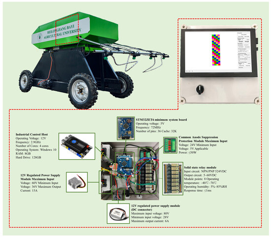
Figure 1. Composition of the Spray Control System.

The lower-level controller utilizes an STM32F103ZET6 minimal system board as its core. It establishes a bidirectional data link with the upper-level computer via the USART serial port, ensuring stable and reliable communication. Upon receiving a spraying command, the controller immediately calculates and outputs precise PWM signals through GPIO. The drive signal first activates a solid-state relay, which then controls the agricultural high-frequency solenoid valve. Each solenoid valve is connected in parallel with a freewheeling diode to absorb reverse electromotive force during shutdown, preventing PCB impact and extending system lifespan.

The core component of the execution unit is the 2W-30-020 “Guardian” agricultural high-frequency solenoid valve, independently developed by the Intelligent Equipment Technology Research Center of the Beijing Academy of Agriculture and Forestry Sciences, with a rated operating voltage of 12 V. Compared to traditional low-frequency solenoid valves, it offers significant advantages in control precision, anti-drip performance, system compatibility, and operational reliability, making it better suited for precision agriculture variable-rate spraying requirements. The flow sensor utilizes the high-precision 938-1538/03 model from Swiss company Digmesa, ensuring accurate flow data acquisition.

2.2. Data Acquisition and Model Construction

To achieve precise tracking of target flow rates under dynamic speeds, the controller primarily calculates the optimal PWM frequency and duty cycle combination in real time based on the target flow rate and actual travel speed. This constitutes a multi-input, multi-output problem with a strongly nonlinear mapping. To quantify the limitations of existing methods, this study first tested an open-loop control strategy based on a preset flow-frequency-duty cycle relationship table on an indoor experimental platform. Under simulated field conditions where speed stepped from 0.5 m/s to 1.5 m/s, the system required over 1.4 s for flow to re-stabilize, with a mean steady-state standard error reaching 18.75%. This demonstrates that traditional linear or decoupled control methods struggle to accurately capture the complex relationships involved. Therefore, this study employs data acquisition to compare existing models and select an optimal control scheme. The goal is to construct a data-driven model with target flow rate and pressure as inputs and PWM parameters as outputs, serving as the core of an intelligent controller.

2.2.1. Data Acquisition and Analysis Palatino Linotype

To investigate the flow rate relationship of the spray system under varying pressure, frequency, and duty cycle conditions, a full factorial design was employed. A spray test bench was constructed based on performance metrics to comprehensively evaluate the effects of pressure P, frequency F, and duty cycle DC on average flow rate Q. Test parameter ranges: P = 0.2, 0.3, 0.4, 0.5 MPa; F = 5, 10, 15, 20 Hz; DC incremented from 10% to 90% in 10% increments. After flow stabilization, each combination was continuously recorded for 30 s, and the average value was taken.

Table 1 evaluates the consistency of spray performance in multi-nozzle systems. Preliminary analysis indicates that experimental data exhibit clear physical patterns. During coordinated multi-nozzle spraying, the coefficients of variation at different pressure levels were 0.0345, 0.0113, 0.0183, and 0.0104 respectively, reflecting excellent consistency. Furthermore, based on single-nozzle flow rate test results, it was found that at a fixed frequency, the spray volume increases significantly with rising pressure, exhibiting a clear positive correlation. Similarly, at a constant pressure, the spray volume also shows a positive correlation with frequency, though this growth trend flattens under high-frequency, high-pressure conditions. The combined results from the charts indicate that spray volume is not determined by a single factor but is jointly regulated by the interactive effects of pressure, frequency, and duty cycle. The relationship between pressure, frequency, and duty cycle is illustrated in Figure 2.

Table 1. Inspection of Spray Consistency for Multiple Nozzles.

Pressure (MPa)	Standard Spray Volume (L/Min)	P1 Spray Volume (L/Min)	P2 Spray Volume (L/Min)	P3 Spray Volume (L/Min)	P4 Spray Volume (L/Min)	Coefficient of Variation
0.2	0.45	0.45	0.475	0.48	0.45	0.0345
0.3	0.55	0.55	0.565	0.56	0.56	0.0113
0.4	0.63	0.62	0.64	0.64	0.62	0.0183
0.5	0.71	0.72	0.73	0.73	0.715	0.0104

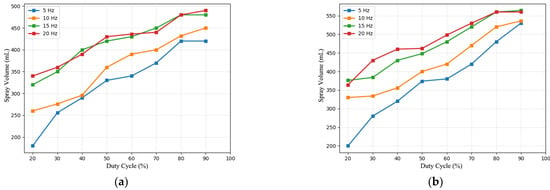
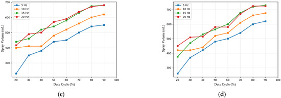
Figure 2. Flow rate as a function of pressure, frequency, and duty cycle. (a) 0.2 Mpa. (b) 0.3 Mpa. (c) 0.4 Mpa. (d) 0.5 Mpa.

2.2.2. Multiple Linear Regression

To establish a preliminary quantitative prediction framework, this study first employs multiple linear regression as the foundational model [12]. An 896-sample dataset was utilized, with its distribution illustrated in Figure 3. Figure 3 shows the distribution of a portion of the dataset. As evident from the figure, data points are distributed relatively uniformly across the frequency and duty cycle ranges, with no noticeable clusters or sparse regions. This indicates that the dataset provides good coverage within these parameter spaces.

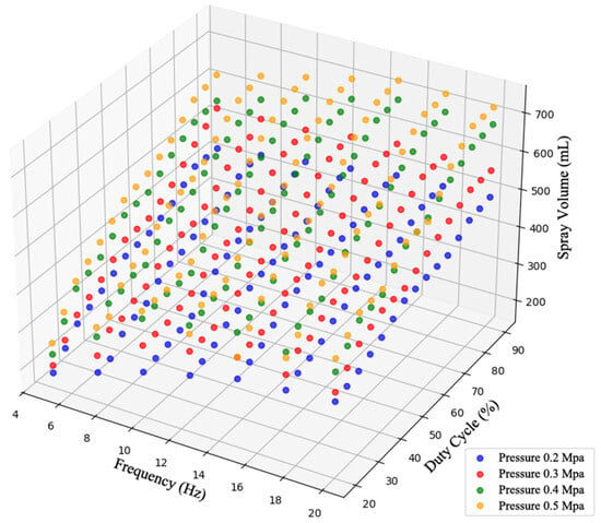
Figure 3. Distribution of the Dataset.

Of these, 807 samples were employed for training, while 89 served as test cases. During the training phase, least squares fitting was applied, incorporating interaction terms between pressure, frequency, and duty cycle to capture coupling effects among parameters. The regression analysis yielded the following fitted equation:

$$Q=-31.0005+582.7321P+8.2107F + 3.5632DC$$

(1)

The model’s statistical metric ${\mathrm{R}}^2=0.939$ indicates good fitting performance on the training data, demonstrating reasonable accuracy in flow prediction. Based on the fitted equation, when we reverse-engineer frequency and duty cycle combinations for a given target flow rate $Q$ using multiple linear regression, it is challenging to precisely determine a unique set of parameters. This difficulty arises because we are solving for multiple unknowns with a single equation. Therefore, we will shift our approach and employ artificial intelligence algorithms to train and test combinations of frequency and duty cycle across different flow rates.

2.2.3. Multi-Model Comparison

Models were refined using artificial intelligence algorithms, comparing standard ANFIS with XGBoost [29], Random Forest [30], and SVM [31] algorithms to predict flow based on input pressure, frequency, and duty cycle for performance analysis. Using the same dataset, the analysis results are shown in Figure 4. Standard ANFIS demonstrated outstanding performance, achieving the highest ${\mathrm{R}}^2$ = 0.9693 on the test set, significantly outperforming other comparison algorithms and exhibiting exceptional generalization capability and model fit. Although ANFIS’s RMSE of 6.3702 is slightly higher than XGBoost and Random Forest, its stable and outstanding performance on both training and test sets demonstrates the algorithm’s robust adaptability and reliability. Notably, ANFIS exhibits the smallest performance discrepancy between training and testing sets, with an R² decrease of only 0.0081—significantly lower than the 0.0361 observed in Support Vector Machines. This indicates ANFIS effectively avoids overfitting issues within limited datasets.

Figure 4. Comparison of Multi-Model Performance.

Continuing the comparative analysis of model back-derivation, we used flow to derive frequency and duty cycle combinations. The comparison revealed that, except for ANFIS, the output processes of other algorithms exhibited limited interpretability. The Random Forest algorithm effectively handles nonlinear relationships, demonstrates low sensitivity to outliers, and exhibits strong resistance to overfitting. XGBoost achieves high accuracy, delivers excellent performance, supports multi-output regression, and shows low sensitivity to missing values. SVM excels on small datasets but suffers from low training efficiency for large-scale data, requires data standardization, is sensitive to parameter and kernel function selection, and offers limited interpretability. ANFIS leverages fuzzy logic interpretability to generate understandable rules, making it particularly suited for control problems and highly compatible with spray application scenarios. Therefore, we selected the ANFIS model for subsequent research.

Standard ANFIS typically comprises five layers: input layer, membership function layer, rule layer, normalization layer, and output layer [32]. The learning process involves two stages: forward propagation and backward propagation. During forward propagation, membership function parameters remain constant while outputs are computed using current parameters, functioning as a fixed fuzzy logic system. Backpropagation calculates the difference between the model output and the target output, then adjusts parameters via gradient descent to minimize error.

To evaluate the fundamental performance of the standard ANFIS architecture in modeling spray systems, a predictive model was constructed with pressure, frequency, and duty cycle as inputs and real-time flow rate as the output. Its performance and residual analysis results are shown in Figure 5. Scatter plots of predicted versus actual values in Figure 5a,b reveal data points clustered closely around the baseline. The model achieved R² values of 0.9774 and 0.9693 on the training and test sets, respectively, with RMSE maintained at a low level. This fully demonstrates the ANFIS model’s exceptional fitting accuracy for complex nonlinear flow relationships. Further residual analysis in Figure 5b,c reveals that errors are randomly and uniformly distributed near the zero line without discernible patterns. Moreover, their frequency distribution in Figure 5d closely matches the standard normal distribution curve. This outcome indicates the absence of systematic prediction bias in the model, confirming a thorough and appropriate fitting process.

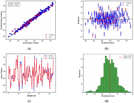
Figure 5. Statistical information of standard ANFIS training data. (a) Actual vs. Predicted. (b) Residual analysis. (c) Test Set: Actual vs. Predicted Comparison. (d) Error Distribution.

2.2.4. Design of the ANFIS Controller

The limitation of the standard ANFIS model lies in its inability to handle multiple outputs. While its strong interpretability enables accurate flow prediction, it cannot forecast frequency duty cycles based on pressure and flow data. Therefore, improvements to the standard ANFIS model are necessary. Two approaches exist for enhancing ANFIS models with multiple outputs [33]: one is the shared premise parameter ANFIS model, and the other is a dual-output ANFIS model. This study tested the dataset using 5-fold cross-validation with 896 data points.

The shared premise parameter ANFIS model employs a four-input, two-output architecture. Due to the limited dataset size, only three Gaussian membership functions—low, medium, and high—were defined for each input. Grid partitioning generated 81 rules. Training employed a hybrid learning algorithm: forward propagation using least squares, backward propagation using gradient descent with a learning rate of 0.01. Mean squared error (MSE) served as the loss function, with a maximum of 4000 iterations and early stopping to prevent overfitting.

Figure 6a’s flow heatmap reveals that spray volume generally increases with rising pressure. At constant pressure, spray volume also rises with increasing frequency. The flow correlation heatmap in Figure 6b reveals strong correlations between spray volume and pressure, frequency, and duty cycle. However, there is minimal correlation between pressure, frequency, and duty cycle. Both analyses show consistent trends: as pressure and spray volume increase, both frequency and duty cycle rise.

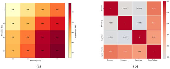
Figure 6. Heatmap of Spray Volume and Spray Volume Correlation. (a) Spray Volume Heat Map. (b) Spray Volume Correlation Heatmap.

By comparing the parameters of the ANFIS model with shared prior parameters and the dual ANFIS model, the results are shown in Figure 7a–c. The mean $R^2$ value of the ANFIS model with shared prior parameters is 0.9414, slightly higher than the 0.9343 of the dual ANFIS model. The shared-prior ANFIS model also exhibited lower average RMSE values for frequency and duty cycle predictions, at 2.9026 and 20.8959 respectively, compared to the dual ANFIS model’s values of 2.9998 and 23.8862.

Figure 7. Cross-validation results for ANFIS with shared premise parameters and dual ANFIS model (5-fold). (a) $R^2$ comparison. (b) Frequency RMSE Comparison. (c) Duty Cycle RMS Comparison.

As shown in Figure 8a,b, both response surfaces illustrate the variation trends of frequency duty cycle combinations under different pressure and spray volume conditions. Comparing the results reveals that the ANFIS controller with shared antecedent parameters and the dual ANFIS model exhibit relatively consistent response trends. However, the response surface of the ANFIS model with shared antecedent parameters shows a greater amplitude of change in the output frequency duty cycle combinations compared to the dual ANFIS model under identical input parameter variations. This indicates higher sensitivity to input parameters in the former model. This difference indicates that in practical applications, the ANFIS model with shared antecedent parameters can more precisely capture the effects of minute changes in input parameters, making it suitable for scenarios requiring high-precision control. Conversely, the dual ANFIS model is better suited for applications requiring a macro-level grasp of trend changes.

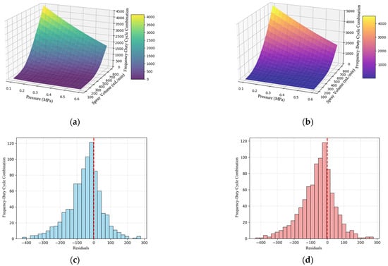
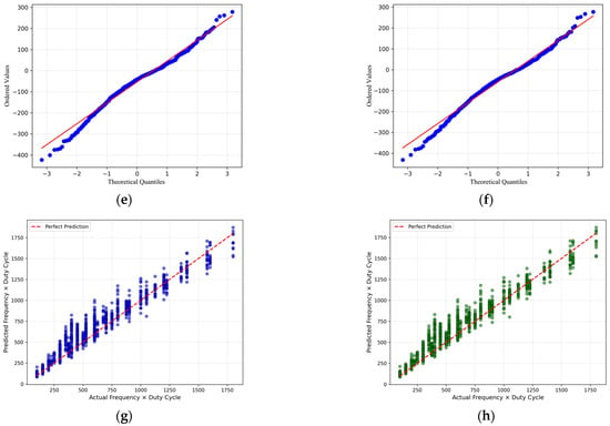
Figure 8. Comparison of Dual ANFIS Model and ANFIS Model with Shared Prerequisite Parameters. (a) Response Surface of the Dual ANFIS Model. (b) Response Surface of ANFIS Models with Shared Prerequisite Parameters. (c) Residual Distribution of the Dual ANFIS Model. (d) Residual Distribution of the Shared Prerequisite Parameter ANFIS Model. (e) QQ Plot of the Dual ANFIS Model. (f) QQ Plot of ANFIS Model with Shared Prerequisite Parameters. (g) Comparison of Prediction Performance Between Dual ANFIS Models. (h) Comparison of Prediction Performance Among ANFIS Models with Shared Input Parameters.

Combining Figure 8c–h, the dual ANFIS output model delivers reliable prediction capabilities across the entire range. The ANFIS model with shared prior parameters demonstrates higher accuracy and stability in prediction performance, particularly suited for scenarios demanding high prediction precision in the low-to-medium value range. Analysis indicates that compared to training two independent ANFIS networks to predict frequency and duty cycle separately, a single large model can automatically learn and coordinate the intrinsic coupling relationship between the two control outputs. This avoids potential command conflicts that may arise from independent models and theoretically offers better convergence and control coordination [34].

As shown in Figure 9, the main improvements to the standard ANFIS model in this study are as follows: by simultaneously processing four related input parameters and sharing premise parameters to output two coupled control commands, it integrates the semantic expression capability of fuzzy logic with the learning ability of neural networks to achieve precise modeling and control of complex nonlinear systems.

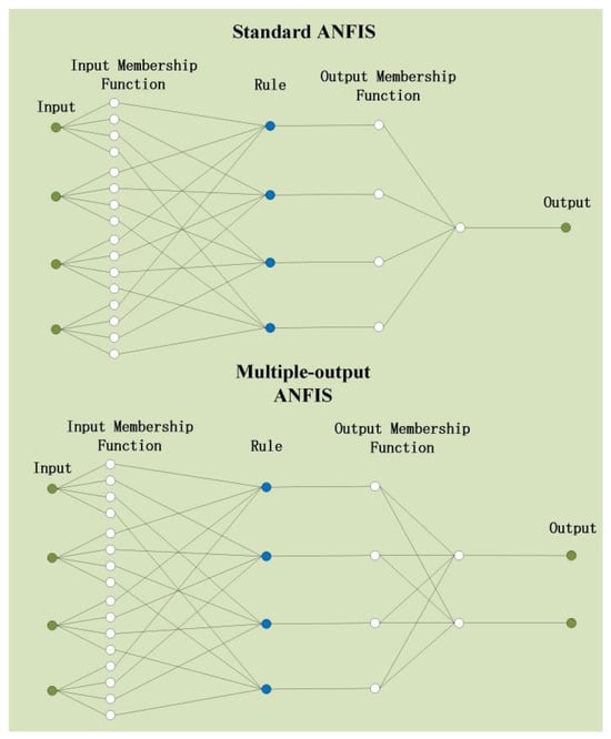
Figure 9. ANFIS Structure for the Spraying System.

Its five-layer structure is largely identical to that of a standard ANFIS, with the primary differences lying in the multi-output linear mapping layer and the overall output layer. The fuzzification layer primarily converts precise numerical inputs into fuzzy semantic values, quantifying the degree to which each input belongs to a specific fuzzy set:

$$O_{1,i} = {\mu }_{A_i}(P)$$

(2)

$$O_{1,j}={ \mu }_{B_j}(F)$$

(3)

$$O_{1,k}={\mu }_{C_k}(D)$$

(4)

$$O_{1,l}={\mu }_{D_l}(Q)$$

(5)

In the membership function layer, Gaussian blurring is applied to perform fuzzy partitioning of the input space. The center and width parameters for the membership functions of pressure, frequency, duty cycle, and flow rate are as follows:

$${\mu }_{A_i}\left(P\right) = \exp \left(-{\displaystyle \frac{(P-c_{P,i}{)}^2}{{\sigma }_{P,i}^2}}\right)$$

(6)

$${\mu }_{B_j}\left(F\right)=\exp \left(-{\displaystyle \frac{(F-c_{F,j}{)}^2}{{\sigma }_{F,j}^2}}\right)$$

(7)

$${\mu }_{C_k}\left(D\right)=\exp \left(-{\displaystyle \frac{(D-c_{D,k}{)}^2}{{\sigma }_{D,k}^2}}\right)$$

(8)

$${\mu }_{D_l}\left(Q\right)=\exp \left(-{\displaystyle \frac{(Q-c_{Q,l}{)}^2}{{\sigma }_{Q,l}^2}}\right)$$

(9)

At the rule layer, the primary evaluation focuses on the activation level of each fuzzy rule under the current input conditions. Each rule corresponds to a fuzzy region within the input space, and the rule strength reflects the degree of match between the current input and that region. The $m$ corresponds to the combination of rules $(i,j,k,l)$:

$$w_m = {\mu }_{A_i}(P)\cdot {\mu }_{B_j}(F)\cdot {\mu }_{C_k}(D)\cdot {\mu }_{D_l}(Q)$$

(10)

The normalization layer converts the absolute trigger strength of each rule into relative weights, ensuring the sum of all weights equals 1 to form a reasonable probability distribution. This normalization operation endows the system with interpolation inference capability. When the input falls within the transition zone of multiple rules, the output becomes a weighted combination of each rule’s conclusion, achieving a smooth input-output mapping. $M$ represents the total number of fuzzy rules in the system, equal to the product of the number of membership functions for each input variable:

$${\overline{w}}_m = {\displaystyle \frac{w_m}{{\sum }_{n=1}^M{w}_n}}$$

(11)

The multi-output linear mapping layer combines normalized rule weights with the corresponding rule’s linear conclusion function to compute each rule’s contribution to the final output. All outputs share the same set of premises, but each rule corresponds to two independent linear conclusion functions:

$$O_{4,m}^F = {\overline{w}}_m\cdot f_m^F = {\overline{w}}_m\cdot (p_m^{F}P +{ q}_m^{F}F + r_m^{F}D + s_m^{F}Q + t_m^F)$$

(12)

$$O_{4,m}^D={\overline{w}}_m\cdot f_m^D={\overline{w}}_m\cdot (p_m^{D}P+{ q}_m^{D}F+{ r}_m^{D}D+s_m^{D}Q+t_m^D)$$

(13)

Among these, $p_m^F$, $q_m^F$, $r_m^F$, $s_m^F$ and $t_m^F$ are linear function parameters for frequency output, while $p_m^D$, $q_m^D$, $r_m^D$, $s_m^D$ and $t_m^D$ are linear function parameters for duty cycle output.

The final output layer aggregates the weighted outputs of all rules to generate the final clarifying control command:

$$F_{out} = {\displaystyle \sum _{m=1}^M}{O}_{4,m}^F ={\displaystyle \sum _{m=1}^M}{\overline{w}}_m\cdot f_m^F$$

(14)

$$D_{out}={\displaystyle \sum _{m=1}^M}{O}_{4,m}^D={\displaystyle \sum _{m=1}^M}{\overline{w}}_m\cdot f_m^D$$

(15)

Among these, $F_{out}$ represents the target frequency value optimized through fuzzy reasoning, while $D_{out}$ denotes the target duty cycle value optimized via fuzzy reasoning. The output result synthesizes knowledge from all activation rules, achieving smooth transitions at rule boundaries and effectively preventing abrupt changes characteristic of traditional controllers.

During the forward propagation phase of the hybrid learning algorithm, the antecedent parameters are fixed, and the optimal consequent parameters are directly computed using the least squares method. This approach yields an analytical solution, exhibits rapid convergence, and offers high computational efficiency. Here, X represents the input data matrix, while YF and YD denote the target output vectors for frequency and duty cycle, respectively:

$${\theta }_{conclusion}^F = (X^{T}X{)}^{-1}{X}^T{Y}_F$$

(16)

$${\theta }_{conclusion}^D=(X^{T}X{)}^{-1}{X}^T{Y}_D$$

(17)

During the backpropagation phase, gradient descent is employed to optimize the prior parameters, progressively adjusting the shape of the membership function:

$$\Delta {\theta }_{premise} = -\eta {\displaystyle \frac{\partial E}{\partial {\theta }_{premise}}}$$

(18)

The error function is

$$E={\displaystyle \frac{1}{2}}[(F_{target}-F_{out}{)}^2+(D_{target}-D_{out}{)}^2]$$

(19)

$\eta$ represents the learning rate, a control parameter that adjusts the step size of parameter updates. Through backpropagation of errors, it optimizes the initial parameters to minimize the multi-objective composite error. Via trial-and-error, the current learning rate is set to 0.01.

2.3. Position Compensation Modeling

By inserting timestamps into the code to measure the execution time of each algorithm module individually, the operational errors in the spraying system primarily stem from three factors: USART transmission delays, positioning information transmission delays, and host computer computation processing delays. Calculations show that the average differences in communication delay, positioning transmission delay, and prescription image calculation delay are 15.89 ms, 108.20 ms, and 5.90 ms, respectively. The GNSS module was configured with a 10 Hz output frequency, theoretically providing a 100 ms refresh cycle. However, field measurements revealed that the complete processing chain—from satellite signal acquisition and decoding to usable coordinate calculation—consistently exceeded this threshold. Multi-scenario testing further confirmed that cumulative delays introduced during signal processing significantly degraded the real-time performance of position data. Additionally, positioning accuracy exhibited dynamic fluctuations, with the amplitude of these variations closely correlated to satellite signal strength. Calculations indicate that in open environments with stable satellite signals, positioning accuracy can reach a minimum of 1.2 m. However, in areas with signal obstruction or severe electromagnetic interference, errors may expand to 5.7 m. Therefore, implementing position compensation becomes a critical measure to mitigate spraying errors caused by delays.

By adding timestamps to capture delay data across all system stages, system delay calibration is completed:

$${\tau }_{\mathit{total}} = {\tau }_{\mathit{GNSS}} + {\tau }_{\mathit{trans}} + {\tau }_{\mathit{proc}} + {\tau }_{\mathit{act}}$$

(20)

${\tau }_{\mathit{GNSS}}$ represents the delay output by the GNSS module, ${\tau }_{\mathit{trans}}$ denotes the serial transmission delay, ${\tau }_{\mathit{proc}}$ indicates the processor computation delay, and ${\tau }_{\mathit{act}}$ signifies the actuator response delay.

Modeling the motion state of the test bench:

$$\left\{\begin{array}{c}\Delta x_k = v_k\Delta t\mathit{cos}{\theta }_k + {\displaystyle \frac{1}{2}}{a}_k{\left(\Delta t\right)}^2\mathit{cos}{\theta }_k\\ \Delta y_k = v_k\Delta t\mathit{sin}{\theta }_k + {\displaystyle \frac{1}{2}}{a}_k{\left(\Delta t\right)}^2\mathit{sin}{\theta }_k\end{array}\right\}$$

(21)

Set up the delay compensation algorithm:

$$\left[\begin{array}{c}{x}_{comp}\\ y_{comp}\end{array}\right] = \left[\begin{array}{c}{x}_{raw}\\ y_{raw}\end{array}\right] + \left[\begin{array}{c}{v}_x{\tau }_{total} + {\displaystyle \frac{1}{2}}{a}_x{\tau }_{total}^2\\ v_y{\tau }_{total} + {\displaystyle \frac{1}{2}}{a}_y{\tau }_{total}^2\end{array}\right] + \lambda \left[\begin{array}{c}{e}_x\\ e_y\end{array}\right]$$

(22)

The geographically compensated coordinates x and y ($x_{comp}$, $y_{comp}$) are adjusted in each iteration using the prediction error e from the previous cycle to correct the current output, thereby suppressing the accumulation of model errors. The feedback correction term is defined as

$$\left[\begin{array}{c}{e}_x\\ e_y\end{array}\right]=\left[\begin{array}{c}{x}_{act}-x_{pred,k-1}\\ y_{act}-y_{pred,k-1}\end{array}\right]$$

(23)

The weight calculation is as follows:

$$\left\{\begin{array}{c}\begin{array}{c}{v}_x = v·\cos \theta \\ v_y = v·\sin \theta \end{array}\\ \begin{array}{c}{a}_x = {\displaystyle \frac{v_k-v_{k-1}}{∆t}}\cos \theta \\ a_y = {\displaystyle \frac{v_k-v_{k-1}}{∆t}}\sin \theta \end{array}\end{array}\right\}$$

(24)

By incorporating an acceleration filter, the current vehicle speed can be simulated to achieve greater accuracy:

$$a_{\mathit{filtered}} = \alpha \cdot a_{\mathit{raw}} + \left(1 - \alpha \right)\cdot a_{\mathit{prev}}$$

(25)

2.4. Spray Control Algorithm

The test platform features three spray operation modes: linked, individual, and prescription map. In linked mode, multiple nozzles share the same set of PWM parameters. Individual mode supports independent frequency and duty cycle settings for any nozzle. Prescription map mode enables precision variable-rate application based on variable values within the map. The prescription map matching algorithm first calculates query results, converts them based on current vehicle speed, and then outputs the optimal PWM frequency and duty cycle combination via the ANFIS algorithm. This combination is parsed into a spray command sequence using flow rate formulas and ultimately transmitted to the lower-level computer for execution. The effective spray width W of the four-nozzle system is set to 2 m. The speed deviation returned by GNSS is converted to km/h units, and the system’s total flow rate is calculated using the following formula:

$$Q ={\displaystyle \frac{q\ast W\ast v}{600}}$$

(26)

where $Q$ represents the total flow rate of the spraying system (L/min), $q$ denotes the application rate per unit area (L/ha), $v$ indicates the velocity data transmitted by the GNSS module (km/h), and $W$ signifies the effective spray width (m).

Figure 10 illustrates the solenoid valve drive circuit structure, with drive control implemented by an STM32 microcontroller. The microcontroller outputs a PWM signal to the relay control terminal, with the coil directly sourced from the microcontroller’s 5 V pin. The load side employs a regulated power supply to step down the input voltage to 12 V. The specific wiring configuration is as follows: The relay’s VCC connects to the microcontroller’s 5 V pin, GND connects to the power supply’s negative terminal, the solenoid valve’s positive terminal connects to the normally closed (NC) contact, and the regulated power supply’s 12 V output connects to the common terminal (COM). When the microcontroller outputs a high level, the relay contact switches to normally open (NO), the 12 V circuit closes, and the valve opens. When the PWM output is low, the contact resets to NC, the circuit breaks, and the valve closes.

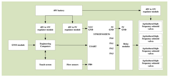
Figure 10. Schematic diagram of variable spraying control system.

As shown in Figure 11, in the prescription map spraying mode, the prescription map is generated by Python in Shapefile format using the WGS-84 coordinate system. The control program first parses the GPRMC message transmitted by the GNSS module. The GPRMC statement contains all core fields required for real-time control of the spraying system, including but not limited to UTC time, latitude/longitude, ground speed, and heading. Fully parsing all NMEA messages would significantly increase unnecessary serial buffer processing time and CPU computational load, compromising control real-time performance. Parsing only GPRMC messages within the real-time control core loop represents an optimal trade-off between meeting control information requirements, ensuring system real-time capability, and reducing implementation complexity. Subsequently, the system acquires real-time latitude/longitude, motion trajectory, and instantaneous velocity from the test platform, invokes the ANFIS controller, and outputs precise frequency and duty cycle commands to the execution unit. Functional modules exchange data via serial bus, with GNSS positioning, flow/pressure data, and control commands transmitted according to standard USART protocols. Flow regulation employs PWM intermittent spray technology. By dynamically adjusting the switching cycle and pulse width of the solenoid valve, the set flow rate is directly mapped to frequency and duty cycle parameters. The controller limits the output frequency duty cycle. Based on the solenoid valve’s maximum response frequency of 20 Hz, the controller’s maximum frequency is capped at 20 Hz. Under flow saturation conditions, the system executes a fully open valve command and records the current anomaly point.

Figure 11. Prescription Map Reading Process.

2.5. Experimental Design

Under simulated field operation conditions, this study designed a mobile robotic platform and conducted variable-speed, variable-rate spraying trials. As shown in Figure 12a, the robot conducts trials based on a predefined prescription map to accurately replicate actual field operation conditions. The prescription map employed a grid size of 3 m × 3 m, with its attribute table containing application rate information for each grid cell. Application rates were divided into five levels, as detailed in Table 2. The trials were conducted at the experimental field of Heilongjiang Bayi Agricultural University.

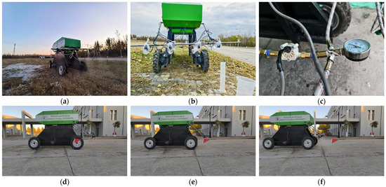
Figure 12. Spray Test. (a) Test site. (b) Pre-calibration. (c) Sensor mounting position. (d) Before entering the target spray zone. (e) While entering the target spray zone. (f) After entering the target spray zone.

Table 2. Spray volume corresponding to the spray grade.

Level	Theoretical Spray Volume (L/Ha)	Theoretical Spray Volume at 1 m/s (L/min)
1	0	0
2	66.7	0.8
3	100	1.2
4	133.3	1.6
5	166.7	2

To enhance the accuracy of flow monitoring in the spray application system, calibration experiments were conducted on the integrated flow sensor. The calibration setup is illustrated in Figure 12b. During calibration, the system flow was regulated using a spray system simulation test bench. A graduated cylinder measured the actual flow rate at the outlet. Simultaneously, the pulse signal output from the flow sensor (Figure 12c) was captured via a data acquisition module, recording the pulse count. Each test group was repeated three times, with the final average value serving as the sensor’s calibration coefficient. As shown in Table 3, the flow sensor’s pulse output coefficient was determined to be 581.38 pulses/L.

Table 3. Sensor check-out.

Test Number	Spray Volume (L)	Number of Output Pulses (Pulses)	Coefficient (Pulses × L−1)	Mean Coefficient (Pulses × L−1)
1	2.56	1491	582.42	581.38
2	3.12	1812	580.77
3	3.41	1981	580.94

As shown in Figure 12d–f, the response delay characteristics under the quantitative prescription map mode were measured repeatedly at constant speed to evaluate the accuracy of the position compensation algorithm. During the test, the spray robot loaded the operational prescription map based on preset parameters. The control system program recorded its latitude and longitude coordinates, speed, and flow rate data every second for subsequent analysis.

3. Results and Discussion

Accuracy test results for the position compensation algorithm indicate the following: at a speed of 1 m/s, the response delay distance when the system enters the prescription map ranges from 22 cm to 35 cm, with an average delay distance of 27 cm (n = 5). Compared to the algorithm without position calibration compensation, the average delay distance is reduced by 33 cm. When the speed increased to 2 m/s, the response delay range expanded to 68 cm to 87 cm, with an average delay distance of 79 cm (n = 5). Compared to the algorithm without position calibration compensation, the average delay distance decreased by 127 cm. This result indicates that the delay compensation algorithm effectively reduces positioning errors.

Based on the comparison of flow rate variation patterns and stability between multi-nozzle and single-nozzle configurations, a spray pressure of 0.3 MPa was selected for the system. The 11,015 nozzle was employed for operations, with the spray robot’s speed limited to 0–9 km/h. During prescription map spraying mode trials, the receiver maintained a stable number of co-visible satellites between 17 and 22 in GNSS mode. The obtained results are shown in Figure 13.

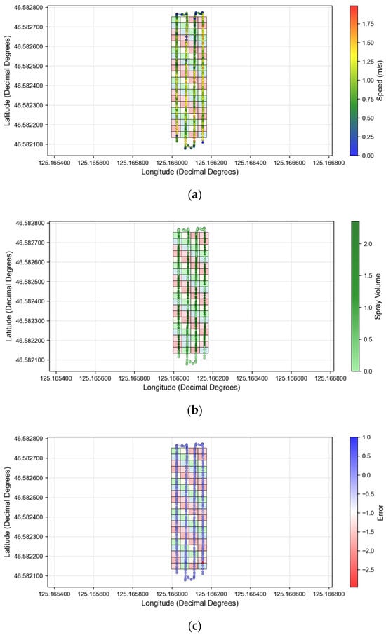
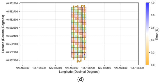
Figure 13. GPS Operation Track. (a) Speed. (b) Spray Volume. (c) Error. (d) Error (%).

Analysis of the instantaneous spray rates across grid intervals within the prescription map reveals that the system accurately controls spray rates under the vast majority of operating conditions. The trial collected 327 raw data points. After validity screening and exclusion of points outside the prescription map, 274 valid samples remained. Spray levels were categorized into five grades, with samples distributed evenly across each grade: Grade 1 (57 samples), Grade 2 (51 samples), Grade 3 (55 samples), Grade 4 (54 samples), and Grade 5 (57 samples). This sample structure provides strong representativeness, objectively reflecting the system’s performance across different spray levels.

Error analysis indicates that the system maintains stable control performance within the primary operating range from Level 2 to Level 5, with average errors of 4.89%, 4.81%, 4.70%, and 5.03%, respectively. All values remain within the ±5% tolerance range. The average errors for speeds less than 0.5 m/s, greater than 0.5 m/s and less than 1 m/s, greater than 1 m/s but less than 1.5 m/s, and greater than 1.5 m/s but less than 2 m/s. The average errors were 5.96%, 4.79%, 4.73%, and 4.84%, respectively, confirming the system’s excellent benchmark flow tracking capability. The standard deviations for levels 2 to 5 were 0.037, 0.0667, 0.1137, and 0.1891, indicating anomalies persist under certain boundary and extreme conditions. By calculating theoretical spray volumes, four false triggers were observed in Level 1, along with 26 flow exceedance points and 7 spray delay points identified across Levels 2–5. Further root cause analysis indicates that errors in Zones 2–4 primarily stem from inherent delays in the GNSS signal reception and processing chain. This causes mismatches between spray commands and real-time positioning. Even with compensation algorithms, minor lags at low speeds or zone transition boundaries may still trigger misalignments. The exceedances in Level 5 were directly linked to system hardware saturation. With a theoretical maximum spray rate of 2.2 L/min, instantaneous flow demands exceeded the solenoid valve’s rated capacity when operating speeds surpassed 1.15 m/s. These phenomena validate the inherent nonlinearity and latency challenges of PWM systems highlighted in the introduction. The improved ANFIS controller in this study optimizes the coordinated output of PWM parameters through data-driven learning, enhancing dynamic response stability. This is reflected in the stable error within primary operational zones. However, it also indicates that compensating for physical limitations of the actuator and absolute latency remains a constraint requiring further breakthroughs in the current solution.

In summary, the system maintains stable control and good accuracy under conventional operating parameters, meeting the basic requirements for variable-rate spraying. However, it is susceptible to position update delays under low-speed boundary conditions and constrained by the response limits of the actuators during high-speed operations. Future research will focus on optimizing position compensation algorithms and actuator selection to further enhance the system’s adaptability across all operating conditions.

4. Conclusions

This study successfully designed and implemented a variable spray control system based on an improved multi-output ANFIS. The main conclusions are as follows.

To meet the demand for precision spraying, this study designed and constructed a prescription-map-based PWM intermittent variable-rate spraying robot platform, completing system parameter testing and calibration indoors.

By comparing the training and validation performance of multiple models on the spraying dataset, the standard ANFIS demonstrated outstanding results due to its high R² value and strong model interpretability. Building upon this, the study further refined the single-output architecture of ANFIS, comparing the performance of a shared-priority-parameter ANFIS controller with a dual-ANFIS controller. The shared-priority-parameter ANFIS controller was selected as the system’s core.

By integrating the delay compensation algorithm with the spray control algorithm, dual-output coordinated optimization of PWM frequency and duty cycle was achieved. Tests conducted at 1 m/s and 2 m/s speeds demonstrated average delay distance reductions of 33 cm and 127 cm, respectively, compared to algorithms without position calibration compensation. This significantly enhances the system’s control performance under nonlinear dynamic conditions.

Field test results demonstrate that the system can maintain steady-state error within ±5.03%. Across varying operating speeds, the average error consistently remains below 5.96%, showcasing rapid and stable response capabilities during stroke speed changes. The standard deviations for primary working ranges 2 to 5 were 0.037, 0.0667, 0.1137, and 0.1891, respectively. Although anomalies may still occur under specific boundary conditions and extreme operating scenarios, this fully integrated hardware-software coordinated spraying robot platform has validated the feasibility and practicality of the solution in actual field operations.

This study retains certain limitations, primarily stemming from the limited scale of the static dataset used for model training, which may impact its generalization capability in more complex and variable field environments. Future work will focus on expanding the experimental dataset’s scale and operational coverage while exploring online learning mechanisms to enable the ANFIS controller to adapt to crop growth cycles and environmental dynamics. Concurrently, the position compensation algorithm will be further optimized to enhance the system’s spraying accuracy and overall adaptability across multimodal, multi-environment, multi-condition, and overlapping scenarios.

References

- Jiao, Y.; Sun, Z.; Jin, Y.; Cui, L.; Zhang, X.; Wang, S.; Zhang, S.; Chang, C.; Ding, S.; Xue, X. Current Status and Future Prospects of Key Technologies in Variable-Rate Spray. Agriculture 2025, 15, 2111. [Google Scholar] [CrossRef]
- Song, Y.; Sun, H.; Li, M.; Zhang, Q. Technology Application of Smart Spray in Agriculture: A Review. Comput. Mater. Contin. 2015, 21, 319–333. [Google Scholar] [CrossRef]
- Fu, Z.T.; Qi, L.J.; Wang, J.H. Developmental Tendency and Strategies of Precision Pesticide Application Techniques. Trans. Chin. Soc. Agric. Mach. 2007, 1, 189–192. (In Chinese) [Google Scholar]
- He, X.K. Research and development of efficient plant protection equipment and precision spraying technology in China: A review. J. Plant Prot 2022, 49, 389–397. (In Chinese) [Google Scholar]
- He, X.K. China Agricultural University Center of Chemicals Application Technology. Research progress and developmental recommendations on precision spraying technology and equipment in China. Smart Agric. 2020, 2, 133–146. (In Chinese) [Google Scholar]
- Dou, H.; Zhang, C.; Li, L.; Hao, G.; Ding, B.; Gong, W.; Huang, P. Application of variable spray technology in agriculture. IOP Conf. Ser. Earth Environ. Sci. 2018, 186, 012007. [Google Scholar] [CrossRef]
- Xu, Y.; Wang, X.; Zhai, Y.; Li, C.; Gao, Z. Precise variable spraying system based on improved genetic proportional-integral-derivative control algorithm. Trans. Inst. Meas. Control. 2021, 43, 3255–3266. [Google Scholar] [CrossRef]
- Yu, Z.N.; Hu, J.; Chu, X.; Liu, C.L.; Liu, Q.L.; Sun, S.Y. Research status and prospect of the spray control method of variable spray system. J. Chin. Agric. Mech. 2019, 40, 72–79. (In Chinese) [Google Scholar]
- Vondricka, J.; Schulze Lammers, P. Measurement of Mixture Homogeneity in Direct Injection Systems. Trans. ASABE 2009, 52, 61–66. [Google Scholar] [CrossRef]
- Robert, P.; Paul, A. Evaluation of Deposition and Application Accuracy of A Pulse Width Modulation Variable Rate Field Sprayer; American Society of Agricultural and Biological Engineers: St. Joseph, MI, USA, 2001. [Google Scholar] [CrossRef]
- Han, S.; Hendrickson, L.L.; Ni, B.; Zhang, Q. Modification and testing of a commercial sprayer with PWM solenoids for precision spraying. Am. Soc. Agric. Biol. Eng. 2001, 17, 591–594. [Google Scholar] [CrossRef]
- Silva, J.E.; Zhu, H.; da Cunha, J.P.A.R. Spray Outputs from a Variable-Rate Sprayer Manipulated with PWM Solenoid Valves. Appl. Eng. Agric. 2018, 34, 527–534. [Google Scholar] [CrossRef]
- Wang, X.D.; Xu, Y.L.; Meng, X.T.; He, R.; Zhai, Y.T. Simulation and experiment of precision variable spraying system based on BAS-PID control. J. Chin. Agric. Mech. 2020, 41, 62–66. (In Chinese) [Google Scholar] [CrossRef]
- Song, L.; Huang, J.; Liang, X.; Yang, S.X.; Hu, W.; Tang, D. An Intelligent Multi-Sensor Variable Spray System with Chaotic Optimization and Adaptive Fuzzy Control. Sensors 2020, 20, 2954. [Google Scholar] [CrossRef]
- Deng, W.; Zhao, C.; Chen, L.; Wang, X. Constant pressure control for variable-rate spray using closed-loop proportion integration differentiation regulation. J. Agric. Eng. 2016, 47, 148. [Google Scholar] [CrossRef]
- Li, K.; Shi, J.; Hu, C.; Xue, W. The Intelligentization Process of Agricultural Greenhouse: A Review of Control Strategies and Modeling Techniques. Agriculture 2025, 15, 2135. [Google Scholar] [CrossRef]
- Yin, Z.; Qian, H.; Xiao, A.; Wu, J.; Liu, G. The Application of Adaptive PID Control in the Spray Robot. In Proceedings of the 2011 Fourth International Conference on Intelligent Computation Technology and Automation, Shenzhen, China, 28–29 March 2011; IEEE: New York, NY, USA, 2011; pp. 528–531. [Google Scholar] [CrossRef]
- Zhang, J.; Yu, Q.; Li, S.; Sun, G. Enhancing position control in pneumatic systems using ANFIS and high-speed on-off valves with compound PWM. Int. J. Hydromechatron. 2024, 1, 347–367. [Google Scholar] [CrossRef]
- Mohandes, M.; Rehman, S.; Rahman, S.M. Estimation of wind speed profile using adaptive neuro-fuzzy inference system (ANFIS). Appl. Energy 2011, 88, 4024–4032. [Google Scholar] [CrossRef]
- Kumar, K.; Das, M.; Karn, A.K. ANFIS robust control application and analysis for load frequency control with nonlinearity. J. Electr. Syst. Inf. Technol. 2024, 11, 65. [Google Scholar] [CrossRef]
- Yaw, O.M.S.; Francis, B.E.; Philip, Y.O. Fractional order ANFIS controllers for LFC in RES integrated three-area power system. J. Electr. Syst. Inf. Technol. 2025, 12, 10. [Google Scholar] [CrossRef]
- Gao, B.; Ma, P.; Hu, G.; Zhong, Y.; Liu, Z. Dual-event-triggering ANFIS-based unscented Kalman filter for cluster cooperative navigation with measurement anomalies. Chin. J. Aeronaut. 2025, 103968. [Google Scholar] [CrossRef]
- Hu, C.; Ru, Y.; Fang, S.; Rong, Z.; Zhou, H.; Yan, X.; Liu, M. Orchard variable rate spraying method and experimental study based on multidimensional prescription maps. Comput. Electron. Agric. 2025, 235, 110379. [Google Scholar] [CrossRef]
- Šarauskis, E.; Kazlauskas, M.; Naujokienė, V.; Bručienė, I.; Steponavičius, D.; Romaneckas, K.; Jasinskas, A. Variable Rate Seeding in Precision Agriculture: Recent Advances and Future Perspectives. Agriculture 2022, 12, 305. [Google Scholar] [CrossRef]
- Karunathilake, E.M.B.M.; Le, A.T.; Heo, S.; Chung, Y.S.; Mansoor, S. The Path to Smart Farming: Innovations and Opportunities in Precision Agriculture. Agriculture 2023, 13, 1593. [Google Scholar] [CrossRef]
- Yao, R.; Xie, B. Intelligent Spraying Robot: Current Status and Future Perspectives from the Perspective of China. Recent Pat. Eng. 2025, 19, E280823220450. [Google Scholar] [CrossRef]
- Wang, F. Control system design of spraying robot. In Proceedings of the 2010 International Conference on Computer and Communication Technologies in Agriculture Engineering, Chengdu, China, 12–13 June 2010; IEEE: New York, NY, USA, 2010; pp. 8–11. [Google Scholar] [CrossRef]
- Du, Y.; Chen, M.; Chen, Z.; Wei, X. Development of vehicular farmland information processing system based on Beidou positioning. In Proceedings of the 2017 4th International Conference on Systems and Informatics (ICSAI), Hangzhou, China, 11–13 November 2017; IEEE: New York, NY, USA, 2017; pp. 99–103. [Google Scholar] [CrossRef]
- Ruggero, G.P.; Anton, C.; Sergio, P.; Christophe, R. Explaining Random Forest and XGBoost with Shallow Decision Trees by Co-clustering Feature Importance. Mach. Learn. 2025, 114, 287. [Google Scholar] [CrossRef]
- Breiman, L. Random Forests. Mach. Learn. 2001, 45, 5–32. [Google Scholar] [CrossRef]
- Chang, C.C.; Hsu, C.W.; Lin, C.J. The analysis of decomposition methods for support vector machines. IEEE Trans. Neural Netw. 2000, 11, 1003–1008. [Google Scholar] [CrossRef]
- Jang, J.S.R. ANFIS: Adaptive-network-based fuzzy inference system. IEEE Trans. Syst. Man Cybern. 1993, 23, 665–685. [Google Scholar] [CrossRef]
- Devi, S.P.; Manivannan, S.; Arunnehru, J. ANFIS Coupled Genetic Algorithm Modelling for MIMO Optimization of Flat Plate Heat Sink; Springer Nature: Singapore, 2023; pp. 597–609. [Google Scholar] [CrossRef]
- Cheng, J.; Guo, Y.; Qian, J. A Multiple Neural Network Architecture Based on Fuzzy C-Means Clustering Algorithm. In Proceedings of the 2006 6th World Congress on Intelligent Control and Automation, Dalian, China, 21–23 June 2006; IEEE: New York, NY, USA, 2006; pp. 1875–1878. [Google Scholar] [CrossRef]
Disclaimer/Publisher’s Note: The statements, opinions and data contained in all publications are solely those of the individual author(s) and contributor(s) and not of MDPI and/or the editor(s). MDPI and/or the editor(s) disclaim responsibility for any injury to people or property resulting from any ideas, methods, instructions or products referred to in the content. |
© 2025 by the authors. Licensee MDPI, Basel, Switzerland. This article is an open access article distributed under the terms and conditions of the Creative Commons Attribution (CC BY) license (https://creativecommons.org/licenses/by/4.0/).