Abstract
Accurately predicting soil particle size fractions (PSFs) and classifying soil texture types are essential for soil resource assessment and sustainable land management. PSFs, comprising clay, silt, and sand, form a compositional dataset constrained to sum to 100%. The practical implications of incorporating compositional data characteristics into PSF mapping remain insufficiently explored. This study applies a two-point machine learning (TPML) model, integrating spatial autocorrelation and attribute similarity, to enhance both the quantitative prediction of PSFs and the categorical classification of soil texture types in the Heihe River Basin, China. TPML was compared with random forest regression kriging (RFRK), random forest (RF), XGBoost, and ordinary kriging (OK), and a novel TPML-C model was developed for multi-class classification tasks. Results show that TPML achieved R2 values of 0.58, 0.55, and 0.64 for clay, silt, and sand, respectively. Among all models, the ALR_TPML predictions showed the most consistent agreement with the observed variability, with predicted ranges of 2.63–98.28% for silt, 0.26–36.16% for clay, and 0.64–96.90% for sand. Across all models, the dominant soil texture types were identified as Sandy Loam (SaLo), Loamy Sand (LoSa), and Silty Loam (SiLo). For soil texture classification, TPML with raw, ALR-, and ILR-transformed data reached right ratios of 61.09%, 55.78%, and 60.00%, correctly identifying 25, 26, and 27 types out of 43. TPML with raw data exhibited strong performance in both regression and classification, with superior ability to separate ambiguous boundaries. Log-ratio transformations, particularly ILR, further improved classification performance by addressing the constraints of compositional data. These findings demonstrate the promise of hybrid machine learning approaches for digital soil mapping and precision agriculture.
1. Introduction
Soil particle size fractions (PSFs) are a critical parameter that characterizes soil physical properties, as it directly influences water retention capacity, aeration, nutrient cycling, and organic matter dynamics []. At the field scale, the spatial distribution of PSFs shows spatial correlation, suggesting that soil texture tends to follow certain spatial patterns, which can provide useful guidance for soil management and land use planning []. Moreover, PSFs play a vital role in regulating soil ecological functions, including nutrient availability, erosion susceptibility [], as well as filtration and buffering processes []. PSFs are widely employed to estimate soil water retention curves, as demonstrated in the work of Haverkamp and Parlange []. Soil texture classification is essential for guiding crop selection and land use planning, as different soil types support different crops due to their distinct physical properties []. It also provides a scientific basis for evaluating land suitability and potential across diverse landscapes []. The Heihe River Basin (HRB) exhibits heterogeneity in land use patterns and soil texture types across its upper, middle, and lower reaches. As a typical ecologically fragile region, it faces long-term challenges such as aridity and soil degradation, making the analysis of PSFs and soil texture types critical for supporting ecological restoration and sustainable land use in the region.
The auxiliary variables were selected following the SCORPAN framework proposed by McBratney et al. [], which extends Jenny’s soil-forming factors into a generic and widely adopted model for digital soil mapping. Li et al. [] revealed that NDVI is closely associated with the spatial distribution of soil texture in their study on permafrost soils in the eastern Qinghai–Tibet Plateau. In addition, topographic factors (including elevation, slope, and aspect) play a crucial role in the formation and distribution of soil texture by regulating vegetation patterns. Significant differences in the generalized fractal dimension (Dq) and single fractal dimension (Dv) of soil particle-size distribution have been observed under different land use types, indicating that land use markedly affects the roughness and heterogeneity of soil texture []. Parent material variation is another key driver of soil texture spatial patterns, often acting in combination with topography and climate []. Classical studies have also demonstrated a strong positive correlation between soil organic carbon (SOC) and the content of clay and silt particles; therefore, SOC is widely regarded as an indirect indicator of soil texture in empirical modeling [].
Various modeling approaches have been employed in the prediction of PSFs and soil texture classification. Traditional geostatistical methods, including ordinary kriging (OK), simple kriging (SK), and inverse distance weighting (IDW), have commonly been applied for spatial interpolation based on autocorrelation structures. However, these methods often lack the flexibility required to integrate high-dimensional environmental covariates. The advent of machine learning (ML) models—such as random forest (RF), Boosted regression trees (BRT), and support vector machines (SVM)—has enabled the modeling of more complex and nonlinear relationships between PSFs and environmental factors. For instance, Liu et al. [] and He et al. [] applied RF and multivariate RF (MRF), respectively, by integrating remote sensing, topographic, and climatic variables to substantially improve PSFs prediction accuracy. In addition, quantile regression forests (QRF) have been employed to quantify prediction uncertainty in PSFs modeling []. Recent studies have demonstrated the effectiveness of combining remote sensing data, terrain parameters, and advanced machine learning (ML) models for soil texture classification. For instance, integrating Landsat 8 spectral bands, terrain attributes, and GLCM texture features with hybrid deep learning models such as RNN-RF has achieved high classification accuracy, with an overall accuracy of 99.2% []. Similarly, SVM, particularly with polynomial kernels, have shown reliable performance in mountainous regions, highlighting the importance of terrain indicators such as elevation and flow path length in soil texture differentiation []. These mainstream ML methods offer distinct advantages in processing high-dimensional auxiliary variables. However, they do not incorporate geographic spatial relationships, which may result in less rational or spatially incoherent predictions [].
Spatial heterogeneity in both PSF distributions and their relationships with covariates—known as dual heterogeneity []—can cause significant prediction errors if neglected. Traditional geostatistical models like OK and IDW rely solely on spatial proximity, while classic machine learning models such as RF and XGBoost use covariate similarity for prediction. Hybrid methods—such as geographically weighted regression (GWR), co-kriging (CK), and random forest regression kriging (RFRK)—combine spatial and attribute information to improve predictions at unsampled locations. For instance, RFRK models trends with RF and residuals with kriging but lacks unified error variance estimation. To address the prediction difficulties caused by dual heterogeneity, Gao et al. [] further developed the two-point machine learning (TPML) model, which integrates spatial autocorrelation and attribute similarity into a high-dimensional feature space, employing a local neighborhood search and pairwise difference learning to enhance prediction accuracy. Built on random forest, TPML also mitigates multicollinearity and overcomes the curse of dimensionality common in local machine learning models. Their results demonstrated that TPML consistently outperformed OK, kriging with external drift, RF, and RFRK. Since its introduction, TPML has been successfully applied in several studies. For example, Wang et al. [] applied TPML to predict soil organic matter (SOM) in Hailun City, Heilongjiang Province, and found that TPML achieved higher accuracy than RF, RFRK, and OK across different sample sizes. Similarly, Qin et al. [] applied TPML in a typical region of the Loess Plateau to predict PSFs using multidimensional auxiliary data, showing that TPML consistently outperformed OK, IDW, RFRK, and RF, with prediction accuracy improving as training data increased. These applications indicate that TPML is effective for spatial prediction of SHM, SOM, and PSFs, with good generalization ability. However, TPML has not yet been applied to the prediction of soil texture types, nor has its potential in multi-class classification tasks been sufficiently explored. To bridge this gap, the present study applies TPML to soil texture type prediction, investigates whether combining TPML with log-ratio transformations can improve both PSF regression and soil texture classification, and further develops an extended model, TPML classification (TPML-C), to explore the applicability of TPML in soil texture type identification.
In this study, soil texture classification was performed based on the United States Department of Agriculture (USDA) system, which has been widely recognized as the standard framework for grading PSFs in soil science [,]. In recent years, significant progress has been made in the development of hybrid modeling approaches that integrate ML techniques with compositional data analysis, geostatistical theory, and large-scale environmental datasets. Studies have shown that models combining log-ratio transformations (e.g., additive log-ratio (ALR), isometric log-ratio (ILR)) with ML or geostatistical techniques (e.g., regression kriging (RK), cokriging (CK)) consistently outperform their non-transformed counterparts in both PSF regression and USDA soil texture classification [,,,]. For example, Li et al. [] and Wang et al. [] reported that ILR-RF and ILR-RK approaches produced more accurate and spatially coherent predictions.
Therefore, this study aims to (1) introduce a new hybrid model framework TPML for the prediction of PSFs and soil texture types, compare it with RFRK, RF, XGBoost, OK to evaluate their performance; (2) systematically investigate the advantages of hybrid modeling approaches that integrate ML, spatial theory, and data transformation techniques for predicting PSFs and classifying soil texture; (3) assess whether log-ratio transformations can enhance prediction accuracy, identify the most influential environmental variables, and analyze their respective effects on PSFs.
2. Materials and Methods
2.1. Overview of the Study Area
The HRB (Figure 1), a representative inland river basin in northwest China [], is situated between 37.57 and 42.82° N and 97.51–102.04° E, spanning Qinghai Province, Gansu Province, and the Inner Mongolia Autonomous Region. It traverses multiple ecological zones, including the Qinghai–Tibet Plateau, the Qilian Mountains, and the Hexi Corridor, and is characterized by a typical continental and arid climate, limited water resources, and intensive land use []. Land use varies across the basin: the southwest is dominated by grassland, forest, and farmland, while the northeast mainly consists of unused land with limited grassland, including sandy land, Gobi, saline-alkali land, marshland, bare land, bare rocky land, and other unused types such as alpine desert and tundra. The upper reaches, within the Qilian Mountain Nature Reserve, have a cold, humid climate and act as key water sources. The middle reaches are arid, with low rainfall (100–250 mm), high evapotranspiration (up to 2000 mm), and average annual temperatures of 6–8 °C; most farmland here depends on irrigation from the Heihe river []. The lower reaches also have an arid climate and rely mainly on animal husbandry []. Water competition, soil degradation, and ecological stress are major challenges in the middle and lower regions []. Due to the region’s ecological diversity, studying soil particle size distribution is important for understanding the interactions between ecological and hydrogeological processes, and for providing a scientific foundation for sustainable land resource management and land degradation prevention in arid regions.
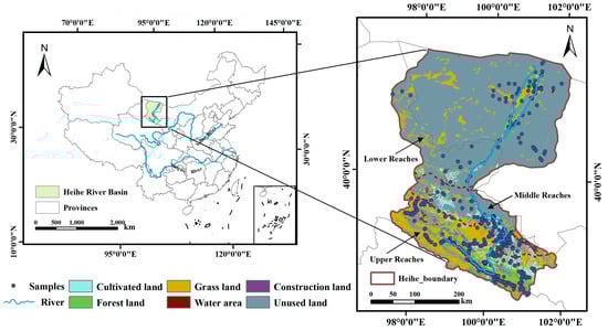
Figure 1.
Overview of the study area.
2.2. Data Source
2.2.1. Soil Sample Data
This study utilized 640 soil sample points collected from the HRB, covering diverse spatial locations characterized by varying topographic, vegetation, soil, human activity, and climatic conditions. Among these, 580 samples (2008–2013) were obtained from the Cold and Arid Regions Science Data Center Regions in China (http://bdc.casnw.net) [,,,,]. At each sampling site, the location was recorded using a handheld global positioning system (GPS) receiver, Garmin Oregon 550t (Garmin International, Olathe, KS, USA). Plant debris and stones were removed, and five subsamples from the 0–20 cm soil layer within a 5 m × 5 m plot were collected, air-dried, and sieved to create a composite sample. An additional replicate composite sample was taken in parallel, and approximately 30 g from each was sent to the laboratory for soil property analysis []. The final soil property values were determined as the average of the two composite samples. The data analysis procedure is informed by methodologies described in [].
2.2.2. Multidimensional Auxiliary Datasets
The auxiliary dataset utilized in this study comprises five categories. All factors were converted into GIS grid maps with a consistent projection and resampled to a uniform spatial resolution of 1 km using the “nearest neighbor” method in ArcGIS 10.8 []. Topographic factors, including elevation, slope, aspect, and curvature, were derived from a 30 m resolution digital elevation model (DEM) obtained from the Shuttle Radar Topography Mission (SRTM, version 4.1) using the Geomorphometry Toolbox in ArcGIS 10.8 []. Landform types were extracted from the 1:1,000,000 scanned and digitized Chinese landform classification map. Vegetation factors: The NDVI was calculated as the 10-year average (2005–2015) from the China Annual Vegetation Index dataset, with a spatial resolution of 250 m. Vegetation types were extracted from the 1:1,000,000 scanned and digitized China Vegetation Map. Soil factors: The SOC content and soil thickness datasets were obtained from the Cold and Arid Regions Science Data Center (http://bdc.casnw.net/) and were provided as simulated grid maps generated through digital soil mapping, with spatial resolutions of 100 m and 90 m, respectively [,]. Soil type information was extracted from a 1:1,000,000 scanned and digitized soil type map of China, which includes Lithosols, Sierozems, Aeolian soils, Fluvo-aquic soils, Frigid felty soils, Frigid frozen soils, Frigid desert soils, Gray-cinnamon soils, and Gray-brown desert soils. Human activity factors: Land use types were derived from 2015 Landsat imagery with a spatial resolution of 1000 m. Climate factors: Annual average precipitation and temperature data were obtained from observations at over 2400 national meteorological stations spanning the past 30 years. The final values represent the averages derived from spatially interpolated results at a spatial resolution of 1 km.
2.3. Model Development
2.3.1. Log-Ratio Transformations
PSFs, comprising clay, silt, and sand, constitute multivariate compositional data characterized by strictly positive components whose sum is constrained to 1 (or 100%). This constant-sum constraint poses challenges for traditional geostatistical methods, which may produce negative predictions or component sums inconsistent with physical reality, thereby violating essential physical constraints []. To address this issue, ALR and ILR transformations are commonly applied in research to map compositional (“closed”) data into real Euclidean space, thereby satisfying the assumptions of traditional statistical modeling [,]. This transformation effectively removes the closure effect’s distortion on the model and ensures both the interpretability and reliability of the prediction results [].
2.3.2. Classic Models
OK Model
This study employs OK, a traditional geostatistical method based on spatial autocorrelation, as a representative technique. Parameters of the random field were estimated from observed data, with weights determined according to spatial autocorrelation quantified by the semivariogram []. Kriging interpolation was conducted using the gstat package in R (v4.4.1) []. The parameters of the OK model are summarized in Table 1.

Table 1.
Variogram model parameters of the OK model.
2.3.3. Machine Learning Models
RF Model
The RF model, derived from the Classification and Regression Tree (CART) algorithm [], addresses CART’s overfitting issue by incorporating the bagging technique []. The model randomly selects a subset of features when splitting nodes to enhance model diversity, reduce feature correlation, and employs out-of-bag (OOB) samples—those not included in the bootstrap sample—to estimate generalization error []. Its advantages include effective prevention of overfitting through dual randomness (sampling and feature selection), insensitivity to noisy data and outliers, and strong robustness. The RF component shares the same parameter settings as the RFRK model. Variable importance is evaluated using the impurity index, and the number of decision trees is set to 250.
XGBoost Model
XGBoost [] is a powerful ML algorithm that employs an ensemble approach, sequentially combining multiple weak learners to improve predictive performance and robustness. Its design specifically addresses two critical challenges in ML: mitigating overfitting via regularization techniques and optimizing computational efficiency [,]. XGBoost employs an iterative additive learning process. Initially, the first base learner is trained on the entire dataset. Subsequent learners are sequentially trained on the residuals of previous predictions, effectively correcting the shortcomings of earlier weak learners []. This iterative refinement continues until predefined stopping criteria are met. The final prediction is obtained by summing the outputs of all individual learners [].
2.3.4. Hybrid Models
RFRK Model
RFRK innovatively integrates ML and geostatistical techniques within its model architecture by employing RF components (via the ranger package in R) [] to capture deterministic trends, and Kriging methods (via the gstat package in R) [] to model residual spatial autocorrelation. The number of decision trees is set to 250. The variogram model parameters are presented in Table 2.
Table 2.
Variogram model parameters of the RFRK model.
TPML Model
The second hybrid model framework is based on the TPML model proposed by Gao et al. []. This framework constructs a weighted high-dimensional feature space, integrates spatial correlation and attribute similarity, and implements a local neighborhood search strategy. Its core objective is to capture complex spatial heterogeneity through differential learning of sample pairs, which can overcome the limitations of traditional distance metrics for categorical variables and address the limitations of conventional models that use equal-weighted nearest neighbor selection. It employs an innovative two-stage modeling strategy:
Firstly, the difference modeling phase: The differences in PSF content between sample points were used as the response variable,
where represents the difference in PSF contents between point and point .
Constructing continuous covariate differences
and type covariate differences
where Equation (2) represents the difference between the k-th continuous covariate at point i and point j. Similarly, Equation (3) represents the vector consisting of the values of the k-th categorical covariate at point i and point j.
Use RF algorithm to train the difference prediction model:
where f represents the supervised learning method, with RF employed in this study; denotes the response variable, which is the difference in PSF contents between training sample point pairs.
Secondly, the spatial prediction stage: For each unobserved point o, the covariate differences between o and all training sample points are calculated, followed by the establishment of a local prediction model:
This implies that by constructing a model between the unobserved point o and the observed point i, the difference in PSF contents between these points can be estimated as:
Here, denotes the estimated PSF content at the unobserved point o to the observed point i. By adding the predicted difference to the known PSF content at observed point , the model derives the predicted PSF content at the unobserved location o, denoted as .
For each target point o in the test dataset, predictions are generated by assessing its relationship with all training points. The final prediction for point o is obtained by averaging the most reliable predictions—those exhibiting the smallest differences—thereby ensuring optimal accuracy.
The original sample was randomly divided into a training set (512 points) and a test set (128 points) at an 80:20 ratio, and the random partitioning was repeated 20 times. The average results from all repetitions were used to calculate the final evaluation metrics. A grid search was conducted on each data partition pair. The parameter for each soil component (sand, silt, and clay) was determined based on the average prediction accuracy across multiple partitions.
TPML-C Model
To expand the applicability of the TPML model in soil texture type identification, this study develops a new classification model, TPML-C, within the TPML framework []. TPML-C retains the original model’s concept of local prediction based on sample differences and introduces adaptive enhancements to the modeling methodology and output mechanism, enabling its suitability for multi-class classification tasks.
In the difference modeling stage, the response variable shifts from a continuous numerical difference to a categorical difference, defined as follows:
were, and denote the class labels of samples i and j, respectively. The difference label serves as the response variable in the difference classification model. Specifically, if two samples belong to the same category, the difference label corresponds to that category. If the categories differ, the difference label represents the transition from to .
In the spatial prediction stage, similar to TPML, for each prediction point o, the covariate differences between o and each training sample point i are computed. The trained difference classification model is then applied to obtain the prediction probability vector for each sample pair:
where represents the covariate difference between point o and training sample i. f(⋅) denotes the trained difference classification model (e.g., RF). is a probability vector over all possible difference labels , with denotes the total number of such labels.
The top- sample pairs ranked by prediction probability are selected to form the neighborhood . Majority voting is then performed on the corresponding predicted labels to determine the final predicted category:
where the value is selected by grid search.
2.4. Model Evaluation Metrics
Mean Absolute Error (MAE), Root Mean Square Error (RMSE), and coefficient of determination (R2) [] are employed to evaluate the accuracy of regression models predicting PSFs. Right Ratio (RR) [], the number of correctly identified classes (NCC), Overall Accuracy (OA), Kappa coefficient, and Average Accuracy (AA) serve as metrics for assessing the overall accuracy of classification models. Additionally, sensitivity, specificity, and balanced accuracy are utilized to evaluate classification accuracy within each category. The specific calculation formulas are as follows:
where is the measured value of soil PSF; is the predicted value; n is the number of validation samples; is the average measured.
where M and n denote the total number of samples and categories in the dataset, respectively. For the i-th feature type, denote the number of reference samples, true positive (TP) samples, and total classified samples (including TP and false positive (FP) samples), respectively. Here, TP indicates correct identification of the i-th feature type, while FP indicates misclassification of other feature types as the i-th type.
2.5. Technical Route
The technical roadmap presented in this study (Figure 2) integrates four key processes: original feature regression modeling, transformed feature regression modeling, direct classification modeling, and comprehensive comparative evaluation.
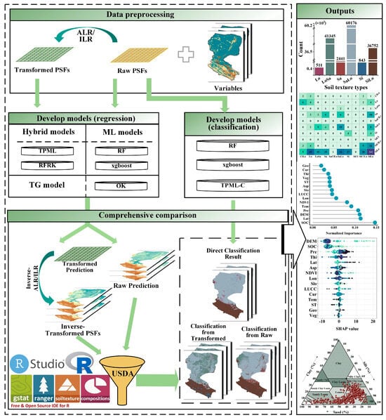
Figure 2.
Experimental flow chart of the case study.
I. Original Feature Regression Modeling Stage
(1) TPML, RF, and RFRK regression models, along with OK and XGBoost, were applied to predict the spatial distribution of silt, clay, and sand content using multidimensional covariate data extracted from sampling points.
(2) The predicted results were classified into soil texture types using the soiltexture package [] in R software.
II. Transformed Feature Regression Modeling Stage
(1) ALR and ILR transformations were applied to the original covariate data.
(2) TPML, RF, and RFRK models were rerun on the transformed data.
(3) Inverse ALR and ILR transformations were applied to the predicted results.
(4) Soil texture classification was performed again using the soiltexture package [].
III. Direct Classification Modeling Stage
(1) The soiltexture package [] was applied to directly classify the covariate values extracted from sampling points.
(2) TPML-C, RF, and XGBoost classification models were run to generate classification results.
IV. Comprehensive Comparison and Verification Phase
(1) Comparison of regression accuracies among different models during the original and transformed feature regression stages.
(2) Systematic comparison of classification accuracies of various models across the three stages: original feature regression, transformed feature regression, and direct classification.
(3) Extraction and analysis of variable importance rankings in the RF and XGBoost models.
3. Results and Analysis
3.1. Descriptive Statistics of Original Data and Transformed Data
Descriptive statistics, including mean, skewness, kurtosis, median, and median absolute deviation (MAD), were calculated for both the original and log-ratio transformed data. Traditional variance analyses, including those based on Euclidean distance, are inappropriate for compositional data like soil PSFs because log-ratio transformations induce geometric asymmetry in the spatial structure []. Consequently, the unbiased total variance [] or robust statistics such as MAD, which are appropriate for compositional data, are employed to characterize the stability or dispersion of the variables. Based on statistical characteristics (Table 3), the mean sand content after transformation (ALR_sand: 28.60; ILR_sand: 28.62) is closer to the median value (24.97) compared to the untransformed mean (30.49). A similar pattern is observed for silt, suggesting that log-ratio transformations mediate the values toward the central tendency, resulting in more balanced distributions. Moreover, the MAD index of ILR is lower than that of ALR (ALR_sand: 1.03; ILR_sand: 0.44) for sand, while slightly higher for silt (ALR_silt: 0.39; ILR_silt: 0.57), indicating that ILR improves the distribution of sand more effectively.
Table 3.
Descriptive statistics for the original and log-ratio-transformed data.
Figure 3 compares the distributions of the original sampling data with those obtained after ALR and ILR transformations. In the original data, silt content primarily ranges from 40% to 80%, with a peak around 60%. Clay content follows an approximately normal distribution, mostly between 0% and 30%, with a peak near 10%, indicating low variability and relative stability across samples. Sand content ranges mainly from 0% to 40%, with a peak around 20%. These patterns suggest that silt is the dominant particle size fraction in the study area. Compared to the original data, the transformed soil component values display more uniform and concentrated distributions. Specifically, the transformed PSFs show a markedly narrower range and reduced variability across components.
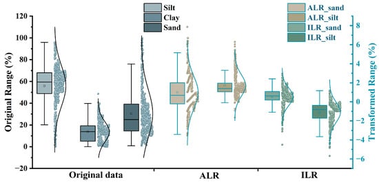
Figure 3.
Comparison of the numerical distribution of the original and log-ratio-transformed data.
3.2. Importance of Environment Variables
Figure 4 illustrates the variable importance rankings obtained from the RF model for predicting PSFs across both original and log-ratio transformed datasets. For the original data, SOC, latitude (Lat), elevation (DEM), precipitation (Pre), and mean annual temperature (Tem) consistently ranked among the top variables, with SOC being most strongly correlated with silt, Lat and Pre with clay, and DEM and SOC with sand. Upon transformation, the importance rankings shift slightly. In the ALR-transformed data, SOC remains dominant for sand, while Pre and Lat gain importance in silt. For the ILR-transformed data, SOC and DEM are particularly important for sand, and Pre and Lat remain top contributors for silt. These patterns suggest that transformations modestly influence the model’s reliance on specific covariates.
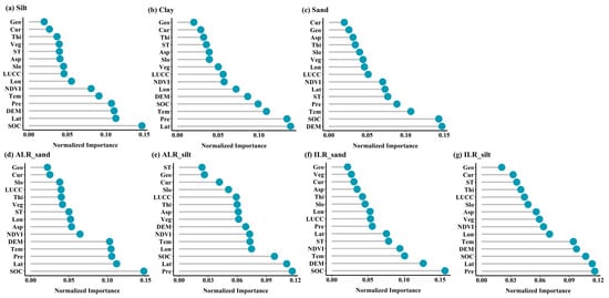
Figure 4.
Variable importance ranking obtained by RF model.
Figure 5 displays SHAP beeswarm plots derived from the XGBoost model, illustrating both the relative importance of variables and the direction of their influence. For the original data, DEM and SOC consistently show the highest contributions across all PSFs, while NDVI and thickness (Thi) exhibit increased importance compared with the RF model. Notably, sand and clay predictions heavily rely on NDVI, which is less emphasized in RF results. For the transformed datasets, SHAP results indicate that DEM, SOC, and NDVI remain consistently among the top features. For example, in ILR_sand, the top features are DEM, SOC, NDVI, aspect (Asp), and slope (Slo), indicating terrain-related covariates gain contributed more significantly after transformation.
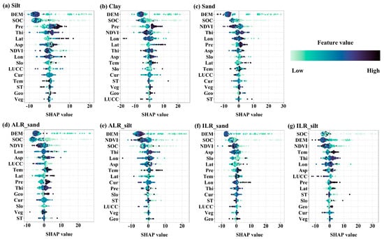
Figure 5.
SHAP beeswarm plot obtained from the XGBoost model.
These findings highlight that while RF and XGBoost both identify DEM and SOC as critical predictors, XGBoost further emphasizes terrain and vegetation indices (e.g., NDVI, Slope, Aspect), especially after transformation. This pattern aligns with findings from other environmental modeling studies using XGBoost. For instance, a recent XGBoost-SHAP analysis in the Jinsha River Basin demonstrated that DEM, slope, aspect, land use, and NDVI are dominant factors driving remote sensing ecological indices []. Additionally, the application of SHAP enhances model interpretability by revealing both the magnitude and direction of each feature’s impact.
3.3. Evaluation of Model Performance Based on Mapping Accuracy
Table 4 summarizes the prediction accuracy of the regression models, classified into three categories: R-H (regression-based hybrid) model, R-ML (regression-based machine learning) model, and R-TG (regression-based traditional geostatistical) model. As shown in Table 4, regression models built using the original, untransformed data generally exhibit higher prediction accuracy than those based on log-ratio transformed data. This suggests that the original sample data exhibit a relatively balanced numerical structure, facilitating more effective direct modeling. In contrast, log-ratio transformations may disrupt this internal balance, leading to reduced model performance. Overall, the two hybrid models, TPML and RFRK, demonstrate superior performance in regression prediction tasks. Specifically, RFRK consistently achieves the highest R2 values across most scenarios, with values reaching 0.63 for sand, 0.58 for clay, and 0.60 for silt, regardless of whether the data are original or transformed (ALR or ILR). TPML demonstrates robust performance in predicting sand content, with R2 values of 0.64 for the original data. followed by 0.63 (RFRK), 0.62 (RF), 0.56 (XGBoost), and 0.56 (OK). Although RFRK achieves the highest R2 values in most scenarios, TPML exhibits competitive or superior performance in terms of error-based metrics. For the original dataset, TPML yields lower MAE and RMSE values for clay content, with 5.14 and 6.37, respectively, than those obtained with RFRK, and achieved a lower RMSE of 13.15 for sand content. These results indicate that TPML not only reduces average prediction errors but also mitigates large deviations, thereby enhancing the overall stability and reliability of predictions for specific PSF components.
Table 4.
Comparison of Regression Accuracy Before and After Transformation Across Different Models.
When using ILR-transformed data, TPML achieves an R2 of 0.60, comparable to the performance of the RFRK and RF models. While RF and XGBoost do not exhibit a definitive advantage in predictive accuracy, their performance remains satisfactory. Furthermore, between the two log-ratio transformation methods, models utilizing ILR transformation generally achieve higher prediction accuracy than those employing ALR transformation. For example, for sand prediction, the RF_ALR and RF_ILR models yield R2 values of 0.57 and 0.60, respectively. This difference can be attributed to ALR transformation utilizing a single component as a reference, constructing an asymmetric log-ratio structure with inconsistent variable scales, which results in greater dispersion of the transformed data (Figure 3). In contrast, ILR transformation constructs an equidistant space using an orthogonal basis, providing improved geometric stability and information retention, thereby rendering the transformed data more suitable for regression modeling. This observation is consistent with the results of Muzzamal et al. [] and Wang et al. [], who explicitly compared ALR and ILR approaches and found that ILR is more stable and generally delivers superior predictive performance.
3.4. Performance Evaluation of Direct Classification Models
Figure 6 presents the confusion matrix heatmaps for three classification models—TPML-C, RF, and XGBoost. The original dataset was randomly partitioned into training and testing subsets using an 80:20 ratio, and this process was repeated five times. The confusion matrices were constructed by aggregating predictions from the five test sets. Overall, all three models exhibit high classification accuracy for the dominant type SiLo, with the RF model performing best. XGBoost successfully identifies eight distinct types, outperforming TPML-C (seven types) and RF (six types). This indicates that the RF model tends to be biased toward the dominant class, resulting in reduced performance on minority types. Regarding specific categories, TPML-C demonstrates superior classification performance for Clay Loam (ClLo) and Silt (Si) types; RF achieves the highest accuracy for SaLo; and XGBoost performs best on Loam (Lo) and LoSa, indicating stronger capability in distinguishing among similar soil texture types.
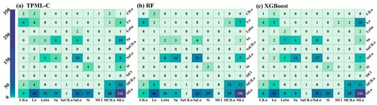
Figure 6.
Confusion matrix heatmaps of TPML-C, RF, and XGBoost.
Table 5 summarizes the classification accuracy metrics for the three models. The OA of the models in the classification task is approximately 60%. The best-performing model is RF, with OA, Kappa, and AA values of 62.19%, 25.35%, and 33.75%, respectively. It outperforms XGBoost and TPML-C in overall prediction accuracy and consistency of type recognition. Its high recognition rate for the dominant type SiLo significantly contributes to the model’s overall accuracy. TPML-C shows slightly lower overall accuracy (59.69%), potentially due to its better preservation of minority type recognition, which may come at the cost of reduced classification stability for some dominant types. XGBoost performs slightly worse than RF in terms of OA and AA but still demonstrates strong classification capability, particularly in recognizing minority types.
Table 5.
Overall classification accuracy of TPML-C, RF, and XGBoost.
Table 6 presents the performance metrics of the TPML-C, RF, and XGBoost models across individual soil texture categories. For the dominant category SiLo, all models exhibited high sensitivity (>0.89), with the RF model achieving a balanced accuracy (BA) of 0.66. TPML-C showed the lowest specificity (0.37) for this category, indicating a tendency to over-predict SiLo instances. For minority categories such as ClLo and Si, TPML outperformed both RF and XGBoost in sensitivity. Its BA for ClLo, Lo, Sa, and Si exceeded that of RF, and in several instances, it outperformed or matched XGBoost, highlighting its enhanced ability to identify rare types. For Silty Clay Loam (SiClLo), RF and XGBoost performed comparably, both achieving a BA of 0.66. Due to the extremely limited number of Sandy Clay Loam (SaClLo) and Silty Clay (SiCl) samples in the test set (only two each), all models were unable to accurately classify these categories (sensitivity = 0, BA = 0.5). Overall, XGBoost demonstrates advantages in balanced accuracy and inter-class balance; TPML-C exhibits potential for identifying minority types; and RF excels in overall accuracy and while preserving inter-class balance.
Table 6.
Accuracy indicators of TPML-C, RF, and XGBoost on various soil texture types.
3.5. Evaluation of Model Accuracy in Predicting Soil Texture Types
Table 7 summarizes the performance metrics of individual models, each aggregated over five independent prediction runs, with the models grouped into five categories: R-H (regression-based hybrid) model, R-ML (regression-based machine learning) model, R-TG (regression-based traditional geostatistical) model, C-H (classification-based hybrid) model and C-ML (classification-based machine learning) model. Among the regression-based prediction models, hybrid models generally outperformed both ML and traditional models in terms of RR and NCC. Specifically, among models using untransformed data, TPML achieved the highest RR (61.09%) and NCC (25). For log-ratio transformed models, RFRK_ILR showed the best performance with the highest RR (63.28%) and NCC (29). The TPML model demonstrated better regression performance (RR: TPML: 61.09%; TPML_ALR: 55.78%; TPML_ILR: 60.00%) on the original data compared to the ALR- and ILR-transformed data. However, the log-ratio transformations enhanced its classification accuracy (TPML_ALR: 26; TPML_ILR: 27). When combining with ILR transformation, both RFRK and RF showed improvements in RR (RFRK_ILR: 63.28%; RF_ILR: 61.09%) and NCC (RFRK_ILR: 29; RF_ILR: 24), indicating enhanced stability and overall performance. For the NCC index derived from the RFRK and RF models using the original dataset (RFRK: 22; RF: 21), the application of ALR transformation led to improvements in classification accuracy, with NCC values increasing to 28 for RFRK_ALR and 26 for RF_ALR. However, this transformation also resulted in a slight decline in regression accuracy, with RR decreasing from 61.09% to 58.44% for RFRK and from 60.47% to 59.53% for RF. XGBoost’s performance on the transformed datasets surpassed that on the original dataset, with the NCC increasing from 21 to 24. The OK model exhibited a slight improvement in type recognition under both ALR and ILR transformations, with the highest NCC observed for OK_ALR (23). However, its RR decreased slightly (OK: 60.63%, OK_ALR: 59.53%, OK_ILR: 60.16%), leading to marginal gains in overall performance. For direct classification models, RF achieved the highest RR (62.66%); however, its NCC value remained relatively low (22), suggesting improved consistency but limited generalization. Although TPML-C produced lower RR values, it identified significantly more soil classes than RF, highlighting its advantage in type coverage. Notably, the XGBoost classification model demonstrated strong performance in both accuracy (RR: 60.94%) and type recognition (NCC: 29), underscoring its effectiveness in soil texture classification. In summary, the log-ratio transformation—particularly the ILR—enhances the ability of each model to recognize soil texture types based on the NCC index, though it often slightly lowers predictive accuracy. Among all models, the hybrid approaches demonstrate the best overall performance, achieving both high RR and NCC on untransformed data, while maintaining strong recognition capability when applied to transformed datasets and classification-based methods. Specifically, among regression models using raw data, TPML attains the highest RR (61.09%) and NCC (25) values, and further improves its NCC to 25 for ALR-transformed data and 27 for ILR-transformed data. RFRK also exhibits a substantial increase in NCC, rising from 22 with raw data to 28 with ALR transformation and 29 with ILR transformation. In comparison, although the RF classification model yields the highest recognition rate (RR), it identifies fewer soil texture types than TPML and XGBoost.
Table 7.
Accuracy of each model in soil texture classification.
Figure 7 presents the USDA texture triangles illustrating soil texture type predictions generated by different models. A comparison of the prediction distributions from the TPML, RFRK, RF, and OK models based on the original data reveals that TPML produces predictions most consistent with the original data’s distribution, followed by RFRK. Predictions from RF and OK are relatively concentrated. In particular, the RF and OK models exhibit a stronger convergence tendency, suggesting that traditional geoscience and ML models may tend to produce conservative predictions under complex spatial heterogeneity, thereby limiting their ability to capture the inherent variability present in the original data. In contrast, hybrid models such as TPML and RFRK demonstrate enhanced capability in replicating the original data distribution. For models based on TPML, the predictions derived from the original data are more clustered, whereas those based on the ALR and ILR transformations are more widely dispersed and more closely resemble the original data’s distribution, especially in the case of TPML_ILR. This indicates that applying ALR and ILR transformations enables the TPML model to predict a broader range of soil texture types.
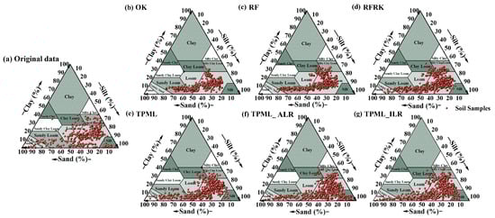
Figure 7.
Predicted soil texture types from USDA texture triangles. Sand, silt, and clay content from (a) original data, (b) OK, (c) RF, (d) RFRK, (e) TPML, (f) TPML_ALR, and (g) TPML_ILR.
3.6. Spatial Distribution Patterns of Sand Content Predicted by Various Models
To analyze the spatial mapping performance of different models, sand content is used as a representative example. Figure 8 presents the spatial distribution of PSF content predicted by the OK, RF, RFRK, and TPML models for gridded test points within the study area. Predictions from the TPML model using ALR- and ILR-transformed data are also included to enable a comparative assessment of the influence of different transformations on the predicted spatial distribution.
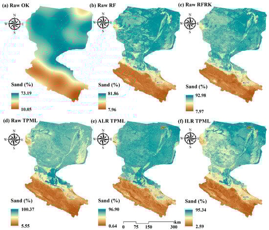
Figure 8.
Sand content maps predicted by different models: OK (a), RF (b), RFRK (c), TPML (d) under original data, and the prediction results after TPML combined with ALR (e) and ILR (f) transformation.
Sand content is low in the upper reaches and high in the lower reaches, consistent with the land use patterns illustrated in Figure 1. This distribution reflects that the upper reaches are dominated by grassland and cultivated land with minimal sand, whereas the lower reaches are characterized by coarser soil textures and are primarily composed of unused land. Sand content near water bodies is generally lower than that in soils farther from the water bodies, indicating finer soil texture adjacent to water sources. Notably, oasis areas in the northeast exhibit markedly lower sand content than their surrounding regions (Figure 8e,f), while the same regions show higher clay content (Figure 9e,f) and lower silt content (Figure 10e,f). This pattern is closely linked to DEM-related variables (slope, aspect, curvature, elevation, thickness) as lower-lying accumulation zones favor the deposition of finer particles like clay, whereas wind erosion processes in exposed areas tend to reduce silt content, consistent with the typical loess-derived soil composition. In contrast, the map based on untransformed data (Figure 8a–d and Figure 10a–d) does not reveal any significant contrast between oasis areas and adjacent soils. This suggests that models employing ALR and ILR transformations are more responsive to variations in soil texture, particularly near oasis areas. This responsiveness is likely due to the effective decoupling of inter-variable dependencies afforded by log-ratio transformations, enhancing the model’s sensitivity to anomalous regions. Conversely, models trained on untransformed data tend to underperform in peripheral and unsampled areas, resulting in conservative predictions that fail to adequately capture the characteristic heterogeneity of oasis areas environments.
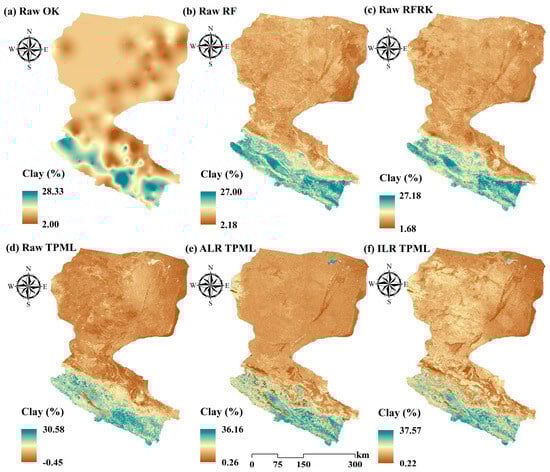
Figure 9.
Clay content maps predicted by different models: OK (a), RF (b), RFRK (c), TPML (d) under original data, and the prediction results after TPML combined with ALR (e) and ILR (f) transformation.
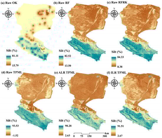
Figure 10.
Silt content maps predicted by different models: OK (a), RF (b), RFRK (c), TPML (d) under original data, and the prediction results after TPML combined with ALR (e) and ILR (f) transformation.
In a localized area of the middle reaches, characterized by high sand content and low silt and clay contents, TPML predictions based on untransformed data produced sand estimates exceeding the theoretical upper bound of 100%, while the corresponding silt and clay estimates fell below 0%, thus violating the constant-sum constraint intrinsic to compositional data. This underscores the importance of applying log-ratio transformations to the original PSF dataset.
Among the transformed models, the ILR-transformed TPML model yields prediction maps with substantially more spatial detail, greater variability, and richer local features compared to those produced by the ALR transformation. This demonstrates that ILR transformation better preserves the geometric structure of compositional data and more effectively reveals spatial heterogeneity of soil texture across regions. Hybrid models such as TPML and RFRK produced finer-grained spatial detail and greater variability, followed by the RF model, while the OK model produced the smoothest predictions. Due to the absence of auxiliary covariate information, the OK predictions lacked spatial detail and reflected only broad regional trends. In terms of prediction range, TPML exhibits the widest range, followed by RFRK and RF, while OK had the narrowest. This further indicates that hybrid models better capture the variability of soil texture properties and produce predictions more closely aligned with the original data distribution (Figure 3).
3.7. Soil Texture Type Prediction Maps of Different Models
Figure 11 compares eight regression models (using raw data, ALR, and ILR transformations) and one classification model in predicting the spatial distribution of soil texture types. Both the direct classification RF model and the TPML regression models (Raw, ALR, and ILR) predicted eight distinct soil texture types—the highest among all models. In comparison, other regression models predicted fewer types: six for Raw RF (Figure 11a) and RF_ILR (Figure 11e), and seven for ALR RF (Figure 11b), RFRK_ALR, and RFRK_ILR. This suggests that post-regression classification tends to exhibit ambiguous type boundaries and limited ability to detect small or marginal texture types. By contrast, TPML regression models (Raw, ALR, and ILR) not only predicted the highest number of texture types but also showed a stronger capacity to resolve finer type variations, highlighting their superior type-level discriminability compared to other regression-based methods. Meanwhile, the direct classification model enables explicit optimization of type boundaries, thereby improving the differentiation of multiple texture types and enhancing the identification and representation of minor types. A statistical analysis of the predicted soil texture distributions across all models reveals that SaLo and SiLo dominate, reflecting the general structure characteristics of soil texture in this region. The raw RF regression model (Figure 11a) showed the strongest capability in identifying major types; however, its ability to detect minor types such as Si and SiClLo was negligible, and its performance in identifying marginal types remained poor. Following log-ratio transformation, both the RF_ALR (Figure 11b) and RF_ILR (Figure 11e) models improved the representation of intermediate types such as LoSa and Sand (Sa). The ALR model notably increased the predicted proportion of LoSa, while the ILR model, although preserving the main type structure, reduced the prediction of minor types (Si, Lo), indicating greater transformation stability. This observation aligns with the results in Table 7: the original RF model was able to identify 21 types, substantially fewer than the RF_ALR (26) and RF_ILR (24) models. The classification RF model also achieved a higher recognition rate (RR) of 62.66%, exceeding that of the three regression RF models (Raw RF: 60.47%; RF_ALR: 59.53%; RF_ILR: 61.09%), indicating that direct classification modeling strikes a more effective balance between accuracy and diversity. Furthermore, the log-ratio transformation contributed to improving the regression model’s ability to represent soil texture types.
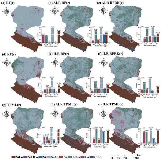
Figure 11.
USDA soil texture classification map. (a,b,e,g–i): Regression prediction results of the RF and TPML models for the original, ALR, and ILR data; (d): Direct classification results of the RF classification model; (c,f): Classification results of the RFRK model combined with ALR and ILR data. Marked (r) is the classification after regression prediction, and (c) is the classification model result.
Compared to the RF and RFRK model, the TPML method showed superior capability in distinguishing soil texture types. On the original dataset, TPML (Figure 11g) predicted eight types and was uniquely able to identify ClLo and Sa. After log-ratio transformation (ALR and ILR), TPML (Figure 11h,i) consistently predicted more texture types than RF (Figure 11b,e) and RFRK (Figure 11c,f), with a distinct advantage in identifying the Si and Lo types. Notably, TPML_ALR and TPML_ILR also provided a clearer delineation of soil texture types near river systems in the eastern region and oasis areas in the northeastern part of the HRB. These findings suggest that TPML benefits from its pairwise learning mechanism, which enhances its sensitivity to attribute differences and spatial heterogeneity, and improves its capacity to detect rare or transitional soil texture types. Additionally, after ILR transformation, the RFRK model (Figure 11f) one additional soil texture type, SiClLo, compared to the RF model (Figure 11e), further demonstrating that incorporating geostatistical structure can enhance the spatial detection of small types.
4. Discussion
4.1. Importance of Environment Variables
Variable importance analysis indicated that SOC, latitude, elevation, average annual temperature, NDVI, and slope contributed most significantly to predicting PSFs in this region. These variables jointly influence soil texture development and distribution through various interacting mechanisms, including soil formation environment, climate gradients, and topographic and geomorphological characteristics. SOC, serving as a comprehensive indicator of soil succession and organic matter accumulation, is closely associated with particle-size-related water retention. Previous studies have demonstrated that SOC content is strongly correlated with soil texture, precipitation, temperature, and soil depth. Notably, clay content is a key determinant of SOC storage, with higher values typically observed in areas receiving more precipitation []. NDVI, as a comprehensive indicator of vegetation cover and health, reflects the feedback mechanisms between soil and vegetation, thereby improving the model’s capacity to capture spatial heterogeneity. Vegetation not only reduces sediment resuspension and enhances sediment retention capacity, but also inhibits surface shortcut flow, thereby improving hydrological efficiency and influencing soil particle size composition and structure []. Within the study area, the upper reaches are dominated by forested land, while the lower reaches are primarily composed of desert and unused land (Figure 1), indicating pronounced spatial heterogeneity along the north–south gradient. This heterogeneity is likely a major driver of variation in soil particle size composition. Latitude and temperature represent primary climatic gradients influencing soil formation. Temperature plays a critical role in shaping the spatial variability of soil composition by influencing processes such as weathering, erosion, and sedimentation. Thermal and moisture conditions drive both physical and chemical weathering, while aeolian processes contribute to the redistribution of clay content []. Latitude, as a critical geographical coordinate, is a major driver of the variation in plant communities observed []. Its high importance among predictive variables also reflects the spatial variability of climatic factors This phenomenon indicates that spatial location, particularly the zonal distribution of climate and vegetation along the latitudinal gradient, plays a critical role in shaping soil composition. Topographic factors, such as elevation and slope, influence sedimentation, erosion, and microclimate distribution, thereby indirectly shaping soil texture patterns. These factors modulate water distribution, erosion intensity, and sedimentation processes, collectively governing the transport and sorting of soil particles. Similarly, Jena et al. [] identified slope and elevation as key determinants influencing PSFs. The spatial distribution of silt is primarily shaped by sedimentation, erosion, and the transport and sorting of soil particles driven by topography, wind, and water [].
Figure 8, Figure 9 and Figure 10 illustrate that the upstream HRB soils are dominated by higher silt and clay but lower sand contents, whereas the downstream soils exhibit the opposite pattern. This spatial distribution is largely controlled by key soil-forming factors, including vegetation cover, topography, and hydrological processes. In the upstream regions, dominated by grasslands and croplands, sand content is relatively low because vegetation cover protects against erosion—by intercepting raindrops, reinforcing soil with roots, and reducing runoff—and steeper topography further enhances the retention of finer particles []. By contrast, the downstream areas are characterized by coarser-textured soils and unused land, where higher sand content results from the preferential deposition of coarse particles and the weaker role of vegetation in stabilizing fine sediments. In addition, sand content near water bodies is generally lower than that in soils farther from the water bodies, which reflects a different depositional environment: in these hydrologically influenced, low-energy settings, fine particles such as silt and clay are more likely to settle, leading to finer soil textures and reduced sand content compared with areas farther from water [].
4.2. Comparison of Different Models for Soil PSFs Mapping
Among spatial prediction models, the two hybrid approaches, TPML and RFRK, demonstrate superior prediction accuracy. Notably, the RFRK and TPML models achieved the highest prediction accuracy when performing regression modeling using the original data. For silt, TPML and RFRK reached R2 values of 0.56 and 0.57, respectively; for clay, both models achieved an R2 of 0.58; and for sand, TPML slightly outperformed RFRK, with R2 values of 0.64 and 0.63, respectively. RFRK utilizes RF to model trends and kriging to interpolate residuals []. Studies have demonstrated that integrating attribute similarity and spatial correlation in hybrid models significantly improves accuracy compared to using RF or OK alone [,]. TPML model incorporates spatial autocorrelation and attribute similarity by embedding them into a high-dimensional space, thereby enabling the assignment of appropriate weights to spatial location covariates and other environmental covariates. Furthermore, TPML overcomes the challenge of computing distances between different categorical variables, effectively enhancing prediction accuracy []. Although RF does not explicitly model spatial correlation, it exhibits advantages in prediction accuracy, primarily due to its strong capacity to handle nonlinear relationships and high-dimensional covariates []. RF can automatically model complex interactions among variables through ensemble learning and possesses strong generalization capabilities. Especially when auxiliary variable information is abundant, RF can fully exploit the explanatory power of covariates on the target variable [], thereby achieving higher prediction accuracy. Although XGBoost did not exhibit outstanding performance in regression modeling, it performed well in the classification task, especially in the recognition of small categories, and maintained a high overall classification accuracy. This advantage can be attributed to its iterative tree structure optimization, which effectively capture nonlinear feature boundaries and improve category discrimination []. In the C-ML models, XGBoost achieved the highest NCC of 29, further demonstrating its robustness and accuracy advantages in multi-category soil texture recognition. In contrast, the OK model, which relies solely on spatial positioning without incorporating auxiliary variables, demonstrates relatively low prediction accuracy due to its inability to capture attribute similarity []. Regarding the spatial distribution of predictions, most models exhibit similar overall trend patterns (Figure 8, Figure 9 and Figure 10). Hybrid models, particularly TPML, generate predictions more consistent with the original data range (Figure 3), yielding more reasonable and detailed predictions. Furthermore, ALR- and ILR-transformed models exhibit heightened sensitivity to spatial heterogeneity, while untransformed models tend to produce conservative predictions. These transformations facilitate the identification of complex spatial variability, a conclusion that is also consistent with the results of Wang et al. []. However, models using untransformed data often achieve higher prediction accuracy than those based on log-ratio-transformed data. In summary, although log-ratio transformation offers theoretical advantages in compositional data analysis by eliminating biases arising from unit and closure constraints, its practical effectiveness in modeling depends on the compatibility between the original data’s distributional structure and the selected model type. Therefore, prior to applying log-ratio transformation, it is essential to assess the distributional characteristics of the original data, carefully weigh the potential benefits and drawbacks, and choose a data processing strategy that optimally fits the specific analytical objective.
4.3. Comparative Analysis of Soil Texture Classification Methods
All three direct classification models demonstrated solid predictive capability for soil texture types, with XGBoost and TPML-C performing particularly well in terms of NCC. Spatially, SaLo and SiLo are dominant across all models. The spatial distribution of the predicted soil texture types aligns well with the distribution patterns of grassland, unused land, and water bodies shown in the land use map (Figure 1). This consistency suggests that the classification results are not only statistically robust but also spatially reasonable, further supporting the validity of the direct classification approach.
Among regression-based reclassification methods, hybrid models significantly outperform traditional spatial classification models, particularly in identifying soil texture types. While RFRK_ILR attains the highest RR and NCC, TPML closely follows with consistently high RR and NCC values, underscoring its robustness and effectiveness in soil texture classification. In contrast, traditional ML models tend to produce conservative predictions, primarily recognizing major types and underrepresenting rare ones. Although OK performs reasonably in RR, it falls short in NCC compared to hybrid and ML models. ALR and ILR transformations enhance the ability to identify marginal types, increasing the number of recognized soil texture types. Hybrid models, particularly TPML, predict the widest range of soil texture types and generate more detailed spatial patterns, reflecting superior performance in capturing complex spatial heterogeneity. Compared to untransformed models, ALR- and ILR-transformed models reveal finer-scale distribution, especially near the northeastern Ejina Oasis area and the upstream forestland regions, where soil properties deviate sharply from surrounding areas [].
Although models using log-ratio transformations generally show slightly lower prediction accuracy than untransformed counterparts, their classification performance improves markedly. ALR-transformed models typically have lower RR values than original models, whereas ILR-transformed models exhibit improved accuracy and type recognition, particularly within the RFRK and RF frameworks. The ILR-transformation combined with RFRK attained the best overall performance, with an RR of 63.28% and 29 out of 43 soil texture types correctly identified—the highest across all models. This suggests ILR transformation better preserves compositional relationships among soil components and enhances model discrimination of complex soil texture types. In particular, when combined with spatial weighting, this approach also yields strong generalizability and interpretability [,,].
4.4. Shortcomings and Prospects of This Article
Sampling points in this study were unevenly distributed across soil textures, with very few for SaClLo and SiCl (4 and 2, respectively) and the majority for SiLo (400 of 640). This imbalance likely constrained the models’ ability to capture differences in PSF contents and affected overall predictive performance. Concentration of samples in upstream areas further limited representation of downstream spatial variability. In addition, the TPML-C model’s computational intensity restricted its scalability for large datasets. Erosion- and transport-related covariates (e.g., flow path length, specific catchment area, flow accumulation) were not included, potentially reducing the models’ capacity to reflect soil redistribution. Repeated random partitioning only partially alleviated sampling bias, and data augmentation strategies (e.g., resampling, bootstrapping, SMOTE) were not employed, though they could enhance training set representativeness and generalization. Future work should aim to balance sample distribution across textures, via stratified sampling, augmentation, or increasing samples for scarce categories. Extending sampling to downstream regions would better capture spatial heterogeneity. Incorporating erosion- and transport-related indices, soil parent material, lithology, mineral composition, and auxiliary datasets (e.g., Landsat 8 spectral bands, large-scale geological maps) could further improve predictive accuracy. Computational efficiency may be enhanced through algorithmic optimization or parallelization. Finally, considering that environmental covariates may introduce errors due to inherent variability, future work could incorporate more soil-specific covariates—such as pH, SOM, K2O, and P2O5—to supplement or partially replace general environmental variables with weaker relevance [].
5. Conclusions
This study systematically evaluated the performance of five regression models (TPML, RF, RFRK, OK, and XGBoost) applied to both raw and log-ratio transformed data, along with three classification methods (TPML-C, RF, and XGBoost), for predicting PSFs in the HRB. The results showed that regression models based on raw data generally achieved higher accuracy than those using ALR- and ILR-transformed data. Among raw-data-based regression models, hybrid models outperformed both traditional ML and classical geoscience models in predictive accuracy, with TPML achieving marginally better results than RFRK in clay and sand content prediction. For soil texture classification, the RF and XGBoost classification models, alongside ILR-transformed TPML and RFRK models, performed well in mean average precision. TPML exhibited distinct advantages in identifying minority types and capturing local spatial variation. Log-ratio transformations, especially ILR, contributed to the improved identification of a broader range of soil texture types, with ILR demonstrating greater stability.
Key predictors influencing the spatial distribution of soil PSFs included SOC, latitude, elevation, and climatic variables such as annual mean temperature, NDVI, and aspect. Data transformations, such as ILR, enhance the model’s ability to capture spatial variation in soil texture compositions. The introduction of TPML-C effectively applies the differential modeling approach that considers spatial autocorrelation and attribute similarity to classification tasks, providing a new way to tackle categorical classification challenges in earth sciences. Despite limitations related to uneven sample distribution and computational efficiency, this study presents a robust modeling framework and theoretical foundation for regional soil texture prediction, offering valuable insights for future soil resource management and ecological conservation.
Author Contributions
Methodology, L.Q. and Z.W.; Validation, L.Q.; Investigation, Z.W.; Writing—original draft, L.Q.; Writing—review and editing, Z.W. and X.Z.; Visualization, L.Q. and X.Z.; Supervision, Z.W.; Project administration, Z.W.; Funding acquisition, Z.W. All authors have read and agreed to the published version of the manuscript.
Funding
This research was funded by National Natural Science Foundation of China, No. 42201518, No. 42401357, Young Elite Scientists Sponsorship Program by BAST, No. BYESS2023005, the Key Program of National Natural Science Foundation of China, No. 42330507 and supported by the Fundamental Research Funds for the Central Universities (2025XJ10).
Data Availability Statement
The data used is primarily reflected in the article. Other relevant data is available from the corresponding author upon request.
Acknowledgments
The authors would like to thank B. Gao [] for his valuable support in implementing and debugging the TPML code throughout this study. The authors also thank Cold and Arid Regions Science Data Center (http://bdc.casnw.net) for providing the dataset information.
Conflicts of Interest
The authors declare no conflicts of interest.
Abbreviations
| HRB | Heihe river basin |
| OK | ordinary kriging |
| RF | random forest |
| RFRK | random forest regression kriging |
| XGBoost | extreme gradient boosting |
| TPML | two-point machine learning |
| TPML-C | two-point machine learning-classification |
| ML | machine learning |
| Geo | geomorphology |
| Cur | curvature |
| Thi | thickness |
| Veg | vegetation |
| ST | soil type |
| Asp | aspect |
| Slo | slope |
| LUCC | land use and land cover |
| Lon | longitude |
| NDVI | normalized difference vegetation index |
| Tem | temperature |
| Pre | precipitation |
| DEM | digital elevation model |
| Lat | latitude |
| SOC | soil organic carbon |
| R-H | regression-based hybrid |
| R-ML | regression-based machine Learning |
| R-TG | regression-based traditional geostatistical |
| C-H | classification-based hybrid |
| C-ML | classification-based machine learning |
| OA | overall accuracy |
| AA | average accuracy |
| RR | right ratio |
| NCC | number of correctly identified types |
| Kurt | kurtosis |
| MAD | median absolute deviation |
References
- Azizi, K.; Garosi, Y.; Ayoubi, S.; Tajik, S. Integration of Sentinel-1/2 and Topographic Attributes to Predict the Spatial Dis-tribution of Soil Texture Fractions in Some Agricultural Soils of Western Iran. Soil Tillage Res. 2023, 229, 105681. [Google Scholar] [CrossRef]
- Delbari, M.; Afrasiab, P.; Loiskandl, W. Geostatistical Analysis of Soil Texture Fractions on the Field Scale. Soil Water Res. 2011, 6, 173–189. [Google Scholar] [CrossRef]
- Gupta, S.; Borrelli, P.; Panagos, P.; Alewell, C. An Advanced Global Soil Erodibility (K) Assessment Including the Effects of Saturated Hydraulic Conductivity. Sci. Total Environ. 2024, 908, 168249. [Google Scholar] [CrossRef]
- Huang, B.; Yuan, Z.; Li, D.; Zheng, M.; Nie, X.; Liao, Y. Effects of Soil Particle Size on the Adsorption, Distribution, and Migration Behaviors of Heavy Metal(Loid)s in Soil: A Review. Environ. Sci. Process. Impacts 2020, 22, 1596–1615. [Google Scholar] [CrossRef]
- Haverkamp, R.; Parlange, J.-Y. Predicting the water-retention curve from particle-size distribution: 1. sandy soils without organic matter: 1. Soil Sci. 1986, 142, 325–339. [Google Scholar] [CrossRef]
- Uddin, M.; Hassan, M.R. A Novel Feature Based Algorithm for Soil Type Classification. Complex Intell. Syst. 2022, 8, 3377–3393. [Google Scholar] [CrossRef]
- Bouma, J.; Bonfante, A.; Basile, A.; van Tol, J.; Hack-ten Broeke, M.J.D.; Mulder, M.; Heinen, M.; Rossiter, D.G.; Poggio, L.; Hirmas, D.R. How Can Pedology and Soil Classification Contribute towards Sustainable Development as a Data Source and Information Carrier? Geoderma 2022, 424, 115988. [Google Scholar] [CrossRef]
- McBratney, A.B.; Mendonça Santos, M.L.; Minasny, B. On Digital Soil Mapping. Geoderma 2003, 117, 3–52. [Google Scholar] [CrossRef]
- Li, W.; Liu, Y.; Wu, X.; Zhao, L.; Wu, T.; Hu, G.; Zou, D.; Qiao, Y.; Fan, X.; Wang, X. Soil Texture Mapping in the Permafrost Region: A Case Study on the Eastern Qinghai–Tibet Plateau. Land 2024, 13, 1855. [Google Scholar] [CrossRef]
- Qi, F.; Zhang, R.; Liu, X.; Niu, Y.; Zhang, H.; Li, H.; Li, J.; Wang, B.; Zhang, G. Soil Particle Size Distribution Characteristics of Different Land-Use Types in the Funiu Mountainous Region. Soil Tillage Res. 2018, 184, 45–51. [Google Scholar] [CrossRef]
- Akpa, S.I.C.; Odeh, I.O.A.; Bishop, T.F.A.; Hartemink, A.E. Digital Mapping of Soil Particle-Size Fractions for Nigeria. Soil Sci. Soc. Am. J. 2014, 78, 1953–1966. [Google Scholar] [CrossRef]
- Hassink, J. The Capacity of Soils to Preserve Organic C and N by Their Association with Clay and Silt Particles. Plant Soil 1997, 191, 77–87. [Google Scholar] [CrossRef]
- Liu, F.; Zhang, G.-L.; Song, X.; Li, D.; Zhao, Y.; Yang, J.; Wu, H.; Yang, F. High-Resolution and Three-Dimensional Mapping of Soil Texture of China. Geoderma 2020, 361, 114061. [Google Scholar] [CrossRef]
- He, W.; Xiao, Z.; Lu, Q.; Wei, L.; Liu, X. Digital Mapping of Soil Particle Size Fractions in the Loess Plateau, China, Using Environmental Variables and Multivariate Random Forest. Remote Sens. 2024, 16, 785. [Google Scholar] [CrossRef]
- Baltensweiler, A.; Walthert, L.; Hanewinkel, M.; Zimmermann, S.; Nussbaum, M. Machine Learning Based Soil Maps for a Wide Range of Soil Properties for the Forested Area of Switzerland. Geoderma Reg. 2021, 27, e00437. [Google Scholar] [CrossRef]
- Suneetha, C.; Kumar, L.; Sreenivas, K.; Mitran, T. Deep Learning-Driven Soil Texture Classifier Using Landsat 8 Images. Remote Sens. Appl. Soc. Environ. 2025, 38, 101568. [Google Scholar] [CrossRef]
- Wu, W.; Li, A.; He, X.; Ma, R.; Liu, H.; Lv, J. A Comparison of Support Vector Machines, Artificial Neural Network and Classification Tree for Identifying Soil Texture Classes in Southwest China. Comput. Electron. Agric. 2018, 144, 86–93. [Google Scholar] [CrossRef]
- Hengl, T.; Nussbaum, M.; Wright, M.N.; Heuvelink, G.B.M.; Gräler, B. Random Forest as a Generic Framework for Predictive Modeling of Spatial and Spatio-Temporal Variables. PeerJ Prepr. 2018, 6, e26693v3. [Google Scholar] [CrossRef]
- Gao, B.; Stein, A.; Wang, J. A Two-Point Machine Learning Method for the Spatial Prediction of Soil Pollution. Int. J. Appl. Earth Obs. Geoinf. 2022, 108, 102742. [Google Scholar] [CrossRef]
- Wang, Y.; Yang, K.; Gao, B.; Feng, A.; Tian, J.; Jiang, C.; Yang, J. Prediction of the Spatial Distribution of Soil Organic Matter Based on Two-Point Machine Learning Method. Nongye Gongcheng Xuebao/Trans. Chin. Soc. Agric. Eng. 2022, 38, 65–73. [Google Scholar] [CrossRef]
- Qin, L.; Wang, Z.; Zhang, X.; Liang, B.; Wang, J. Optimization of Soil Particle Size Mapping Incorporating Spatial Autocorrelation and Attribute Similarity. IEEE J. Sel. Top. Appl. Earth Obs. Remote Sens. 2025, 18, 21044–21064. [Google Scholar] [CrossRef]
- Staff, S.S. Soil Survey Manual; U.S. Department of Agriculture, Handbook 18: Washington, DC, USA, 2017; ISBN 978-0160942855. [Google Scholar]
- Wikipedia Contributors Soil Texture. Available online: https://en.wikipedia.org/wiki/Soil_texture (accessed on 2 August 2025).
- Li, J.; Wan, H.; Shang, S. Comparison of Interpolation Methods for Mapping Layered Soil Particle-Size Fractions and Texture in an Arid Oasis. CATENA 2020, 190, 104514. [Google Scholar] [CrossRef]
- Wang, C.; Zhao, L.; Fang, H.; Wang, L.; Xing, Z.; Zou, D.; Hu, G.; Wu, X.; Zhao, Y.; Sheng, Y.; et al. Mapping Surficial Soil Particle Size Fractions in Alpine Permafrost Regions of the Qinghai-Tibet Plateau. Remote Sens. 2021, 13, 1392. [Google Scholar] [CrossRef]
- Zhang, M.; Shi, W.; Ma, Y.; Ge, Y. Mapping Soil Particle-Size Fractions Based on Compositional Balances. CATENA 2024, 234, 107643. [Google Scholar] [CrossRef]
- Wang, Z.; Shi, W.; Zhou, W.; Li, X.; Yue, T. Comparison of Additive and Isometric Log-Ratio Transformations Combined with Machine Learning and Regression Kriging Models for Mapping Soil Particle Size Fractions. Geoderma 2020, 365, 114214. [Google Scholar] [CrossRef]
- Li, X.; Cheng, G.; Ge, Y.; Li, H.; Han, F.; Hu, X.; Tian, W.; Tian, Y.; Pan, X.; Nian, Y.; et al. Hydrological Cycle in the Heihe River Basin and Its Implication for Water Resource Management in Endorheic Basins. J. Geophys. Res. Atmos. 2018, 123, 890–914. [Google Scholar] [CrossRef]
- Wang, C.; Jiang, Q.; Shao, Y.; Sun, S.; Xiao, L.; Guo, J. Ecological Environment Assessment Based on Land Use Simulation: A Case Study in the Heihe River Basin. Sci. Total. Environ. 2019, 697, 133928. [Google Scholar] [CrossRef]
- Huo, L.; Xie, Q.; Sun, L.; Song, L.; Tao, S.; Liu, S.; Wang, Z.; Li, Y. Estimation of Agricultural Flood Irrigation Water Consumption in the Heihe River Basin, China, Using Satellite Based Daily Land Surface Evapotranspiration and Soil Moisture. J. Hydrol. Reg. Stud. 2025, 60, 102524. [Google Scholar] [CrossRef]
- Song, X.; Xu, Z. Table of Value Input-Output of 42 Departments in Gansu Lingao Region in the Middle Reaches of Heihe River (2012); National Tibetan Plateau Data Center: Beijing, China, 2015. [Google Scholar]
- Jiang, Y.; Xu, X.; Huang, Q.; Huo, Z.; Huang, G. Assessment of Irrigation Performance and Water Productivity in Irrigated Areas of the Middle Heihe River Basin Using a Distributed Agro-Hydrological Model. Agric. Water Manag. 2015, 147, 67–81. [Google Scholar] [CrossRef]
- Ma, M.; Wang, X.; Wang, H.; Yu, W. HiWATER: Dataset of Soil Parameters in the Midstream of the Heihe River Basin (2012); National Tibetan Plateau Data Center: Beijing, China, 2013. [Google Scholar]
- Song, X.-D.; Brus, D.J.; Liu, F.; Li, D.-C.; Zhao, Y.-G.; Yang, J.-L.; Zhang, G.-L. Mapping Soil Organic Carbon Content by Geographically Weighted Regression: A Case Study in the Heihe River Basin, China. Geoderma 2016, 261, 11–22. [Google Scholar] [CrossRef]
- Pan, J.; Zhao, S. WATER: Dateset of Soil Texture Measurements in the Biandukou and A″rou Foci Experimental Area on 9 October 2008; National Tibetan Plateau Data Center: Beijing, China, 2014. [Google Scholar] [CrossRef]
- Wang, Z.; Shi, W. Robust Variogram Estimation Combined with Isometric Log-Ratio Transformation for Improved Accuracy of Soil Particle-Size Fraction Mapping. Geoderma 2018, 324, 56–66. [Google Scholar] [CrossRef]
- Environmental Systems Research Institute. Esri ArcGIS Desktop: Release 10.8; Environmental Systems Research Institute: Redlands, CA, USA, 2020. [Google Scholar]
- Reuter, H.I.; Nelson, A. Chapter 11 Geomorphometry in ESRI Packages. In Developments in Soil Science; Hengl, T., Reuter, H.I., Eds.; Elsevier: Amsterdam, The Netherlands, 2009; Volume 33, pp. 269–291. ISBN 0166-2481. [Google Scholar]
- Yang, R.-M.; Zhang, G.-L.; Liu, F.; Lu, Y.-Y.; Yang, F.; Yang, F.; Yang, M.; Zhao, Y.-G.; Li, D.-C. Comparison of Boosted Regression Tree and Random Forest Models for Mapping Topsoil Organic Carbon Concentration in an Alpine Ecosystem. Ecol. Indic. 2016, 60, 870–878. [Google Scholar] [CrossRef]
- Walvoort, D.J.J.; de Gruijter, J.J. Compositional Kriging: A Spatial Interpolation Method for Compositional Data. Math. Geol. 2001, 33, 951–966. [Google Scholar] [CrossRef]
- Muzzamal, M.; Huang, J.; Nielson, R.; Sefton, M.; Triantafilis, J. Mapping Soil Particle-Size Fractions Using Additive Log-Ratio (ALR) and Isometric Log-Ratio (ILR) Transformations and Proximally Sensed Ancillary Data. Clays Clay Miner. 2018, 66, 9–27. [Google Scholar] [CrossRef]
- Niang, M.; Nolin, M.; Jégo, G.; Perron, I. Digital Mapping of Soil Texture Using RADARSAT-2 Polarimetric Synthetic Aperture Radar Data. Soil Sci. Soc. Am. J. 2014, 78, 673–684. [Google Scholar] [CrossRef]
- Webster, R. Is Soil Variation Random? Geoderma 2000, 97, 149–163. [Google Scholar] [CrossRef]
- Pebesma, E.J. Multivariable Geostatistics in S: The Gstat Package. Comput. Geosci. 2004, 30, 683–691. [Google Scholar] [CrossRef]
- Breiman, L. Random Forests. Mach. Learn. 2001, 45, 5–32. [Google Scholar] [CrossRef]
- Breiman, L. Bagging Predictors. Mach. Learn. 1996, 24, 123–140. [Google Scholar] [CrossRef]
- Liaw, A.; Wiener, M. Classification and Regression by randomForest. R News 2002, 2, 18–22. [Google Scholar]
- Chen, T.; Guestrin, C. XGBoost: A Scalable Tree Boosting System. In Proceedings of the 22nd ACM SIGKDD International Conference on Knowledge Discovery and Data Mining, San Francisco, CA, USA, 13–17 August 2016. [Google Scholar]
- Fan, J.; Wang, X.; Wu, L.; Zhou, H.; Zhang, F.; Yu, X.; Lu, X.; Xiang, Y. Comparison of Support Vector Machine and Extreme Gradient Boosting for Predicting Daily Global Solar Radiation Using Temperature and Precipitation in Humid Subtropical Climates: A Case Study in China. Energy Convers. Manag. 2018, 164, 102–111. [Google Scholar] [CrossRef]
- Wang, Y.; Sun, S.; Chen, X.; Zeng, X.; Kong, Y.; Chen, J.; Guo, Y.; Wang, T. Short-Term Load Forecasting of Industrial Customers Based on SVMD and XGBoost. Int. J. Electr. Power Energy Syst. 2021, 129, 106830. [Google Scholar] [CrossRef]
- Zhao, Z.; Yang, W.; Zhai, Y.; Liang, Y.; Zhao, Y. Identify DNA-Binding Proteins Through the Extreme Gradient Boosting Algorithm. Front. Genet. 2022, 12, 821996. [Google Scholar] [CrossRef]
- Wright, M.N.; Ziegler, A. Ranger: A Fast Implementation of Random Forests for High Dimensional Data in C++ and R. J. Stat. Softw. 2017, 77, 1–17. [Google Scholar] [CrossRef]
- Wang, Z.; Shi, W. Mapping Soil Particle-Size Fractions: A Comparison of Compositional Kriging and Log-Ratio Kriging. J. Hydrol. 2017, 546, 526–541. [Google Scholar] [CrossRef]
- Moeys, J.; Shangguan, W.; Petzold, R.; Minasny, B.; Rosca, B.; Jelinski, N.; Zelazny, W.; Souza, R.M.S.; Safanelli, J.L.; ten Caten, A. Comprehensive R Archive Network (CRAN). Soiltexture: Functions for Soil Texture Plot, Classification and Transformation; R Foundation: Vienna, Austria, 2024. [Google Scholar] [CrossRef]
- Filzmoser, P.; Hron, K.; Reimann, C. Univariate Statistical Analysis of Environmental (Compositional) Data: Problems and Possibilities. Sci. Total Environ. 2009, 407, 6100–6108. [Google Scholar] [CrossRef] [PubMed]
- Pawlowsky-Glahn, V.; Egozcue, J.J.; Tolosana Delgado, R. Lecture Notes on Compositional Data Analysis; Universitat de Girona: Catalonia, Spain, 2007; Available online: http://hdl.handle.net/10256/297 (accessed on 8 September 2025).
- Xia, J.; Zhang, G.; Ma, S.; Pan, Y. Spatial Heterogeneity of Driving Factors in Multi-Vegetation Indices RSEI Based on the XGBoost-SHAP Model: A Case Study of the Jinsha River Basin, Yunnan. Land 2025, 14, 925. [Google Scholar] [CrossRef]
- Deliboran, A. Carbon and Nitrogen Stocks of Olive Orchard Soils in Izmir Province. J. Tekirdag Agric. Fac. Tekirdag Ziraat Fak. Derg. 2024, 21, 111–124. [Google Scholar] [CrossRef]
- Braskerud, B.C. The Influence of Vegetation on Sedimentation and Resuspension of Soil Particles in Small Constructed Wetlands. J. Environ. Qual. 2001, 30, 1447–1457. [Google Scholar] [CrossRef]
- Fanfarillo, E.; Petit, S.; Dessaint, F.; Rosati, L.; Abbate, G. Species Composition, Richness, and Diversity of Weed Communities of Winter Arable Land in Relation to Geo-Environmental Factors: A Gradient Analysis in Mainland Italy. Botany 2020, 98, 381–392. [Google Scholar] [CrossRef]
- Jena, R.K.; Moharana, P.C.; Dharumarajan, S.; Sharma, G.K.; Ray, P.; Deb Roy, P.; Ghosh, D.; Das, B.; Alsuhaibani, A.M.; Gaber, A.; et al. Spatial Prediction of Soil Particle-Size Fractions Using Digital Soil Mapping in the North Eastern Region of India. Land 2023, 12, 1295. [Google Scholar] [CrossRef]
- Sun, C.; Hou, H.; Chen, W. Effects of Vegetation Cover and Slope on Soil Erosion in the Eastern Chinese Loess Plateau under Different Rainfall Regimes. PeerJ 2021, 9, e11226. [Google Scholar] [CrossRef]
- Pan, Y.; Zhang, H.; Li, X.; Xie, Y. Effects of Sedimentation on Soil Physical and Chemical Properties and Vegetation Characteristics in Sand Dunes at the Southern Dongting Lake Region, China. Sci. Rep. 2016, 6, 36300. [Google Scholar] [CrossRef]
- Xu, J.; Zhang, F.; Ruan, H.; Hu, H.; Liu, Y.; Zhong, K.; Jing, W.; Yang, J.; Liu, X. Hybrid Modelling of Random Forests and Kriging with Sentinel-2A Multispectral Imagery to Determine Urban Brightness Temperatures with High Resolution. Int. J. Remote Sens. 2021, 42, 2174–2202. [Google Scholar] [CrossRef]
- Ho, V.H.; Morita, H.; Bachofer, F.; Ho, T.H. Random Forest Regression Kriging Modeling for Soil Organic Carbon Density Estimation Using Multi-Source Environmental Data in Central Vietnamese Forests. Model. Earth Syst. Environ. 2024, 10, 7137–7158. [Google Scholar] [CrossRef]
- Ho, V.H.; Morita, H.; Ho, T.H.; Bachofer, F.; Nguyen, T.T. Comparison of Geostatistics, Machine Learning Algorithms, and Their Hybrid Approaches for Modeling Soil Organic Carbon Density in Tropical Forests. J. Soils Sediments 2025, 25, 1554–1577. [Google Scholar] [CrossRef]
- Canero, F.M.; Rodriguez-Galiano, V.; Aragones, D. Machine Learning and Feature Selection for Soil Spectroscopy. An Evaluation of Random Forest Wrappers to Predict Soil Organic Matter, Clay, and Carbonates. Heliyon 2024, 10, e30228. [Google Scholar] [CrossRef] [PubMed]
- Sakhaee, A.; Gebauer, A.; Liess, M.; Don, A. Spatial Prediction of Organic Carbon in German Agricultural Topsoil Using Machine Learning Algorithms. Soil 2022, 8, 587–604. [Google Scholar] [CrossRef]
- Qin, F.; Guo, C.; Liu, D.; Xu, S.; Wang, S. A Comparison of Ordinary Kriging, Regression Kriging and REML-EBLUP for Mapping Soil Organic Matter on a Regional Scale. Arab. J. Geosci. 2022, 15, 1120. [Google Scholar] [CrossRef]
- John, K.; Bouslihim, Y.; Isong, I.A.; Hssaini, L.; Razouk, R.; Kebonye, N.M.; Agyeman, P.C.; Penížek, V.; Zádorová, T. Mapping Soil Nutrients via Different Covariates Combinations: Theory and an Example from Morocco. Ecol. Process. 2022, 11, 23. [Google Scholar] [CrossRef]
Disclaimer/Publisher’s Note: The statements, opinions and data contained in all publications are solely those of the individual author(s) and contributor(s) and not of MDPI and/or the editor(s). MDPI and/or the editor(s) disclaim responsibility for any injury to people or property resulting from any ideas, methods, instructions or products referred to in the content. |
© 2025 by the authors. Licensee MDPI, Basel, Switzerland. This article is an open access article distributed under the terms and conditions of the Creative Commons Attribution (CC BY) license (https://creativecommons.org/licenses/by/4.0/).