Abstract
Precise monitoring of vegetative growth is essential for assessing crop responses to environmental changes. Conventional methods of geometric characterization of plants such as RGB imaging, multispectral sensing, and manual measurements often lack precision or scalability for growth monitoring of rice. LiDAR offers high-resolution, non-destructive 3D canopy characterization, yet applications in rice cultivation across different growth stages remain underexplored, while LiDAR has shown success in other crops such as vineyards. This study addresses that gap by using LiDAR for geometric characterization of rice plants at early, middle, and late growth stages. The objective of this study was to characterize rice plant geometry such as plant height, canopy volume, row distance, and plant spacing using the proximal LiDAR sensing technique at three different growth stages. A commercial LiDAR sensor (model: VPL−16, Velodyne Lidar, San Jose, CA, USA) mounted on a wheeled aluminum frame for data collection, preprocessing, visualization, and geometric feature characterization using a commercial software solution, Python (version 3.11.5), and a custom algorithm. Manual measurements compared with the LiDAR 3D point cloud data measurements, demonstrating high precision in estimating plant geometric characteristics. LiDAR-estimated plant height, canopy volume, row distance, and spacing were 0.5 ± 0.1 m, 0.7 ± 0.05 m3, 0.3 ± 0.00 m, and 0.2 ± 0.001 m at the early stage; 0.93 ± 0.13 m, 1.30 ± 0.12 m3, 0.32 ± 0.01 m, and 0.19 ± 0.01 m at the middle stage; and 0.99 ± 0.06 m, 1.25 ± 0.13 m3, 0.38 ± 0.03 m, and 0.10 ± 0.01 m at the late growth stage. These measurements closely matched manual observations across three stages. RMSE values ranged from 0.01 to 0.06 m and r2 values ranged from 0.86 to 0.98 across parameters, confirming the high accuracy and reliability of proximal LiDAR sensing under field conditions. Although precision was achieved across growth stages, complex canopy structures under field conditions posed segmentation challenges. Further advances in point cloud filtering and classification are required to reliably capture such variability.
1. Introduction
Rice (Oryza sativa L.) is one of the most significant staple crops, serving as a primary food source for over half of the global population [,]. Over 50% of the population of the world consumes rice as a staple food []. Effective field management is essential for maximizing crop yield and precise monitoring of rice vegetative growth for understanding phenological development and informing data-driven agronomic decisions. It is crucial for understanding plant responses to environmental changes at different growth stages. Measurement of key vegetative growth parameters such as canopy height (CH), canopy volume, row distance, and plant spacing is vital for optimizing field management and improving yield predictions [,]. Geometric plant features are widely recognized for their influence on rice yield potential [,]. Proximal sensing technologies refer to non-contact sensing methods that collect detailed information about crops from a short distance, typically within a few meters. Advancements in proximal sensing technologies have contributed to precision agriculture by identifying optimal methods for crop-specific applications []. These technologies are often mounted on ground-based platforms such as tractors, handheld rigs, tripods, or robots and are used directly in the field.
Crop geometry is the arrangement of plants in different rows and columns in an area to efficiently utilize natural resources []. Traditionally, crop geometric characterization has relied on manual measurements [,], which, despite their continued use, are prone to inaccuracies, labor-intensive procedures, and time constraints []. Furthermore, manual plant feature characterization requires skilled labor [,]. In large-scale fields, manual sampling is often performed on a small subset of plants, leading to potential errors when extrapolating results to entire fields []. Selecting a precise and reliable sensing technology is crucial for accurate vegetative growth monitoring. Although high-resolution sensor data can enhance measurement accuracy, the associated costs and complex data processing requirements may outweigh the benefits for certain agricultural applications []. Therefore, sensor selection should align with specific objectives in precision agriculture while balancing accuracy, cost, and data-processing efficiency.
Sensor selection in unstructured environments is particularly challenging due to the complexity of plant and crop geometry []. In precision agricultural operations, appropriate sensing techniques are necessary to ensure reliable and accurate measurements. The rapid development of three-dimensional (3D) sensing technologies has improved high-throughput height measurements []. Crop height is a fundamental indicator of growth status, typically measured from the soil surface to the top of the plants, and can serve as an alternative method for biomass estimation []. Traditional destructive methods for determining the leaf area index (LAI) are labor-intensive and impractical for large-scale sampling. Although non-destructive LAI estimation methods have been developed, they remain prone to operator-induced measurement errors, and no standardized technique exists for non-destructive crop LAI estimation throughout the entire growing season []. Additionally, the relationship between LAI and vegetation height varies across plant types and growth stages [,]. The integration of multiple sensors and techniques is often required to achieve accurate measurements of plant geometric characteristics, while a single sensor cannot comprehensively capture all plant geometric characteristics.
LiDAR is a prominent sensor for high-precision measurements, enabling non-invasive 3D data acquisition using narrow laser beams. This makes it highly suitable for crop phenotyping [] and detailed canopy structure analysis []. While UAV-based photogrammetry can also generate 3D point clouds comparable to those obtained from LiDAR [,], the point cloud density from photogrammetry depends on image resolution and overlap. While photogrammetry is generally more cost-effective than LiDAR [], ground-mounted LiDAR typically produces denser 3D point clouds compared to UAV-derived datasets []. UAV imagery has demonstrated reliability in plant canopy characterization for crop growth monitoring [,]. However, combinations of sensing technologies, including RGB cameras [], ultrasonic sensors [], multispectral and hyperspectral sensors [], and laser scanners [], have been used to characterize crop canopies [].
Stereo vision has also been utilized to capture detailed 3D plant structures using multiview images []. However, these methods face challenges such as stereo matching errors under varying illumination, incomplete reconstructions due to occlusions, and trade-offs between accuracy and efficiency []. Unlike RGB-D cameras, stereo cameras passively determine depth by identifying common pixels in consecutive frames and measuring their displacement, which is inversely proportional to the distance of the objects from the sensor []. These systems perform well in outdoor conditions, providing high-resolution depth measurements that remain robust under varying lighting conditions. However, they also present challenges such as correspondence errors and high computational demands []. Although depth cameras have improved in resolution, they still struggle in brightly lit environments [,,,]. Compared to expensive laser-based systems and gaming sensors such as the Kinect (Microsoft, Redmond, WA, USA), which have limited range and perform poorly under high illumination [], stereo vision remains a cost-effective alternative for generating high-resolution 3D point clouds. The integration of 3D spatial data with color information enhances segmentation accuracy during point cloud preprocessing.
Proximal sensing technologies, including LiDAR, enable the capture of high-resolution images with spatial resolutions below 1 cm, making them suitable for distinguishing individual plant organs []. While aerial remote sensing faces challenges in achieving this level of detail, recent advancements have improved the ability to detect fine plant features []. Ultrasonic sensors are cost-effective and simple to operate but suffer from reduced measurement accuracy and susceptibility to environmental interference. Spectral imaging provides valuable texture and reflectance information but lacks the structural detail necessary for comprehensive plant morphology assessment []. Optical imaging methods can extract 3D features effectively in controlled settings but struggle with full plant architecture reconstruction in outdoor environments []. Recent advances in LiDAR technology have facilitated the acquisition of high-resolution 3D structural data for agricultural applications. Consequently, LiDAR has gained increasing interest in plant geometric features characterization []. LiDAR mounted on UAVs or ground sensing platforms has been used to assess the geometric characterization of crops such as peanuts, maize, and fruit trees [,,]. However, rice crops, which become denser in the middle to late growth stages, present challenges for measuring row distance and plant spacing due to leaf overlap []. Additionally, rice is often cultivated in flooded paddies, posing accessibility challenges for conventional ground sensing platforms, while water-filled channels and uneven terrain can interfere with LiDAR operation []. Furthermore, UAV-generated airflow can disturb the canopy structure, affecting data consistency []. Compared to airborne LiDAR, terrestrial laser scanning (TLS) offers a cost-effective and user-friendly solution for acquiring high-density, accurate, and repeatable data. This makes it particularly suitable for monitoring specific crops and has led to widespread use in the precise extraction of geometric features of individual crops []. Considering these complexities, mobile terrestrial laser scanning (MTLS) techniques have been increasingly adopted due to their improved plant geometric characterization as well as measurement reliability of vegetative growth monitoring parameters.
Based on recent advancements in viticulture research [,], the advantages of proximal LiDAR sensing are emphasized, including the ability to accurately capture plant structure in complex field conditions. Although LiDAR has been used for high-resolution 3D canopy characterization in other crops, such as vineyards [,], at high resolutions, the use of it in rice cultivation across different growth stages remains limited. Specific gaps include the lack of studies capturing the structural dynamics of rice throughout the early, middle, and late growth stages; the challenges posed by dense leaf overlap and flooded paddies; the absence of standardized high-precision protocols for extracting key geometric traits such as canopy height, canopy volume, row distance, and plant spacing; and the lack of comparative assessments between LiDAR-derived metrics and traditional manual methods for rice growth monitoring. To address these limitations, this study focused on enhancing the accuracy and consistency of vegetative growth monitoring in rice cultivation across different growth stages by introducing the systematic use of terrestrial LiDAR for extracting high-resolution geometrical characteristics throughout the growth cycle. Therefore, the objective was to characterize geometric features of rice plants using the proximal LiDAR sensing for monitoring vegetative growth at three vegetative growth stages.
2. Materials and Methods
2.1. LiDAR Sensor Selection and Rice Field Selection
In this study, a commercial LiDAR (model: VPL−16, Velodyne Lidar, San Jose, CA, USA) was used for data collection, and the detailed specifications are shown in Table 1. The LiDAR sensor is capable of scanning distances up to 100 m, providing sufficient coverage for the rice field. It is designed for efficiency with low power usage, a lightweight design, a compact size, and single and dual return functionality. It is equipped with 16 scanning channels, enabling it to collect approximately 300,000 data points per second. This high point density is critical for achieving accurate and detailed measurements of plant height, canopy volume, and other geometric features of rice plants. It provides a 360° horizontal field of view and a 30° vertical field of view, with a ±15° vertical tilt, allowing for a diverse scanning range, which is important for capturing data from different angles in a rice field, especially when the plants are densely packed. It enables the collection of comprehensive data over a wide area. It is highly suitable for several applications such as autonomous vehicles, robotics, and terrestrial 3D mapping in precision agriculture for the characterization of plant features. Despite having visible rotating parts, it demonstrates strong durability and reliable performance over a wide range of temperatures. The sensor provides detailed and high-resolution 3D data of the surrounding environment. The data was collected in a rice field located at Jeollabukdo Agriculture Research and Extension Services, Iksan, Republic of Korea. Figure 1 shows the rice field for LiDAR data collection. This site was selected as a representative rice field condition, providing an ideal setting for testing and validating the use of LiDAR sensors in estimating and analyzing the geometric features of rice plants. LiDAR data was collected from a selected rice plot that was 12 m long and 8 m wide in size.

Table 1.
Technical specifications of the LiDAR sensor used in this study [].
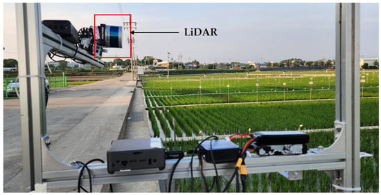
Figure 1.
Selected LiDAR and rice field for LiDAR data collection.
2.2. Sampling Strategy
To capture the variability in rice plant structures, a systematic sampling strategy was employed. Twenty data frames were selected from the acquired data frames exhibiting diverse plant heights, shapes, and sizes. For geometric feature characterization, these data frames were captured from six consecutive rice plant rows, exhibiting different sizes and shapes to represent the variability of the rice plant geometric features. This allowed for comprehensive analysis and ensured that the results were representative of the diversity under field conditions. The plant rows selected for data collection were aligned with the field layout, and a region of interest (ROI) of 1 m by 0.9 m was segmented from each data frame for further analysis.
No experimental treatments, such as different rice varieties or fertilization regimes, were implemented in this study, as the primary goal was to validate LiDAR sensor technology across rice plants in a natural, unmodified field setting. The selected sampling method aimed to capture multiple growth stages (early, middle, and late) of the rice plants to assess the performance of LiDAR in monitoring plant development over time.
2.3. Data Collection with Customized Structural Platform
Point cloud data were collected using a proximal LiDAR sensor. The LiDAR was mounted on a custom aluminum frame designed for stable movement along rails between field plots. All necessary components such as LiDAR sensor, terminal box, GPS, battery, microcontroller, display monitor, mounts, and wheels are detailed in the schematic provided in Figure 2. The sensor height was kept at 80 cm above the crop canopy, adjustable according to growth stage. During scanning, the structure was manually moved at walking speed to maintain data quality. A small region of interest (ROI) of 1 m by 0.9 m was segmented from each frame for data processing and measurements. The LiDAR, aligned vertically, captured 360° point cloud data to assess plant height, canopy volume, row distance, and plant spacing. Data acquisition covered six rows, and Python was used for analysis.

Figure 2.
Customized structure used for LiDAR point cloud data collection in the rice field. The setup includes the following components: LiDAR sensor, LiDAR terminal box, GPS module, battery, micro-controller (data processing unit), display monitor, data collection frame, adjustable mounts, wheels, and railroad for guided movement.
Figure 3 illustrates the sensor setup used to collect high-resolution 3D point cloud data of rice plants through proximal LiDAR sensing. A commercial LiDAR sensor was mounted on a customized mobile frame and integrated with essential components for field operation. The sensor was connected to a terminal box, which distributed power and enabled communication between the LiDAR and a compact data processing unit. Two 12 V batteries powered the entire system, ensuring portability and continuous operation in field conditions. The terminal box also stabilized power supply and managed data transmission via a high-speed Ethernet connection. Real-time visualization of LiDAR scans was possible through an attached display monitor, and a USB drive was used to store the collected data. This configuration allowed close-range scanning of rice crop geometry with precise spatial detail, enabling accurate measurement of plant structure under actual field conditions. Additionally, an external GPS unit (model: GPS18x LVC, Garmin, Martinez, CA, USA) was used for accurate geolocation and data synchronization.
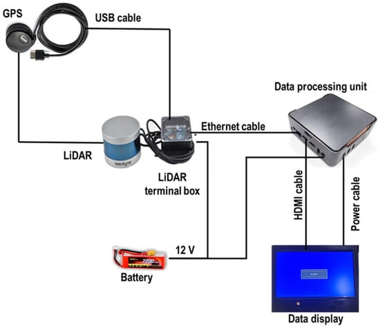
Figure 3.
Sensor setup for data acquisition in this study.
Commercial software (model: Veloview, Ver 5.1.0, Kitware, Inc., Clifton Park, NY, USA) was used for data acquisition, visualization, and analysis of LiDAR data. Visualization of distance measurements as point cloud data was allowed by the software, which offered customizable color maps for variables consisting of laser ID, intensity of return, dual return type, azimuth, time, and distance. The software also supports data export in CSV format (x, y, z coordinates). In combination with Python, it facilitated comprehensive 3D point cloud processing and analysis. The software facilitated further data visualization, analysis, and measurement, as described by Zulkifli et al. []. Figure 3 presents a schematic diagram of this configuration, detailing how each component was integrated to optimize data collection and system performance.
Manual measurement in the field is shown in Figure 4. A measuring ruler was used for collecting manually measured plant height, canopy volume, row distance, and plant spacing, as shown in Figure 5. The measurement started from the soil surface at the base of the stem to the highest point of the canopy, usually the tip of the flag leaf. The leaves were not lifted or extended. To obtain accurate results, three representative plant hills were selected from each region of interest, and the average manual measurement height was calculated. To ensure a good representation of overall canopy conditions, the plant height was estimated from data points of each synchronized data collection region of interest. For manual measurement, the vertical distance from the ground to the top of the canopy was measured using the measuring tape, as shown in Figure 4a. The individual height measurements were then recorded for further analysis and to compare with the LiDAR measurement of plant height. Similarly, to obtain accurate measurement results of the canopy volume, representative sample plots were selected within each region of interest, and the average canopy volume was calculated. The canopy volume was calculated by multiplying the average height by the plot area while considering the lateral spread of the canopy and the density, as shown in Figure 4b. This process involved a combination of direct measurements and visual estimations, where the recorded measurements were used for further analysis and comparison with LiDAR measurement of canopy volume, as shown in Figure 5. However, no formal record was kept regarding the observer bias during the visual estimation process. While it was likely that some level of bias should have been introduced due to the subjective nature of visual estimations, it was unable to quantify or measure that bias due to the lack of recorded observations. Consequently, it was unable to provide a specific error estimate. Future work could benefit from a more structured approach, including recording observations and assessing potential bias, to better understand and account for estimation errors.

Figure 4.
Manual measurement of rice plant geometric features. (a) plant height; (b) canopy volume; (c) row and plant distance.
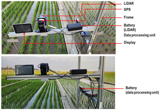
Figure 5.
Point cloud data acquisition in rice field using proximal LiDAR sensing.
2.4. Plant Geometric Feature Characterization from LiDAR Data
A Python program was developed to manage data processing, visualization, and the characterization of rice plant features for vegetative growth monitoring. The data processing workflow included steps such as data conversion, targeted data frame selection, outlier removal, down-sampling, denoising, ground point removal, voxelization, and the preparation of three-dimensional point cloud density (PCD) maps. Data analysis was performed to estimate and interpret the results. Data acquisition started with a LiDAR sensor, which captured 3D point cloud data from a rice field. The raw point cloud data captured by the LiDAR was stored in a PCAP file format.
Point cloud data processing algorithms for the visualization of the point cloud and extraction of measurement data for vegetative growth monitoring of rice are shown in Figure 6. The data processing pipeline begins with importing essential Python libraries and defining custom functions for convex hull volume calculation and 3D visualization of LiDAR point cloud data. A LiDAR point cloud (PCD) file is loaded and validated to ensure the presence of valid data. The data is then converted into a structured format suitable for numerical analysis. Spatial dimensions such as height, width, and depth are computed, followed by the calculation of geometric features including average plant spacing and row distances. A convex hull is then computed to estimate the canopy volume. The point cloud data undergoes preprocessing, including outlier removal, noise reduction, and downsampling. Downsampling is performed using a voxel grid technique, where the point cloud is divided into small cubic units, or voxels. For each voxel, a representative point is selected, typically by averaging the points within that voxel. This reduces the overall number of points in the dataset while preserving key features of the plant canopy structure. The downsampling process minimizes computational load, making it more efficient to handle large point cloud datasets while maintaining the necessary resolution for accurate canopy feature extraction. Voxelization segments the data, and a convex hull is computed to visualize the plant canopy.
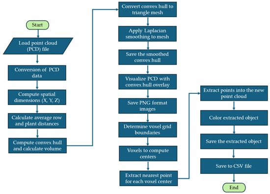
Figure 6.
Flow chart of point cloud data processing algorithms for the visualization of the point cloud and extraction of measurement data for vegetative growth monitoring.
To generate the convex hull boundary, the QuickHull algorithm was used. The algorithm begins by selecting two extreme points, typically with the minimum and maximum values along one dimension, which define a line segment that forms part of the convex hull. The remaining points were then divided into two subsets, one on each side of the line segment. For each subset, the farthest point from the line or plane was identified, and that point became part of the convex hull. The farthest point, along with the original two points, formed a new triangle or tetrahedron, which was added to the hull. The process continued recursively, checking the points outside the current shape and adding the farthest points to the hull. This iterative process continued until no more points could be added, at which point the algorithm terminated, resulting in a minimal convex shape that enclosed all the points. Subsequently, the convex hull was converted into a triangular mesh and smoothed using Laplacian filtering. The convex hull was smoothed using Laplacian filtering to refine the mesh, which was then visualized over the original point cloud. The smoothed hull was saved and visualized with the original point cloud as an overlay, and the visualizations were exported in PNG format. After that, a voxel grid was created by defining grid boundaries and computing voxel centers. For each voxel center, the nearest point from the original point cloud was extracted to build a representative object point cloud. The extracted objects were then colored, saved as a new point cloud, and exported as both image and CSV files. The entire workflow facilitated an automated, detailed, and accurate characterization of rice canopy structures, enabling further quantitative analysis and detailed growth monitoring.
2.4.1. Plant Height and Canopy Volume
Figure 7 illustrates the workflow for processing LiDAR point cloud data and extracting two key parameters of vegetative growth monitoring of rice, namely plant height and canopy volume. The data procedure begins with data collection and conversion, where the LiDAR sensor captured data in a pcap (packet capture) format that stored the raw laser returns, and the pcap files were then converted into PCD (point cloud data) files, enabling point cloud data preprocessing and allowing each PCD file to be parsed for (x, y, z) coordinates. In the data preprocessing stage, the 3D point clouds were structured into a format suitable for further analysis, with a region of interest (ROI) segmentation removing background objects or untargeted ground points, followed by denoising algorithms to eliminate noise and outliers, radius outlier removal to remove inconsistent points beyond typical density thresholds, and voxel grid downsampling to reduce overall point density while retaining essential structural features. The coordinates of the point cloud data were transformed to adjust the data for further processing in the step of transforming each coordinate of point cloud data. The transformation was involved in aligning the data with a specific reference frame or correcting for any distortions. The points that did not represent the objects of interest (rice plants) were removed from the data, particularly the ground plane during the removal of the untargeted points (ground plane). Through outlier removal, the outlier points were eliminated as they were significantly different from most of the data, potentially due to noise or errors during data acquisition. The ground sampling process involved sampling the ground data to further refine the dataset by focusing on relevant points. Noise within the point cloud data was reduced to improve the accuracy and clarity of the data, particularly focusing on removing irrelevant data points in the denoising step. In the ground removal step, the ground points were hidden or excluded from the dataset to focus on the rice plants by hiding the ground. For the extraction of plant data, data points were selected from the region of interest of plants only without the ground through hiding the ground and automatically segmented using Python code. After the ground was hidden, the dataset contained only the points that represented the rice plants. The selected points were then used to prepare a 3D point cloud density map, visually representing the density and distribution of the points that prepared the rice plants for visualization.
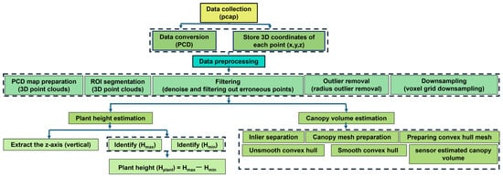
Figure 7.
Data processing and measurement of sensor estimated plant height and canopy volume.
Using Python codes, the rice plant metrics such as height and canopy volume were estimated. The data was preprocessed to meet the requirements of the intended applications. Plant height estimation was performed by isolating the vertical (z) axis, identifying the minimum (Hmin) and maximum (Hmax) z-values to represent ground level and the highest point of the canopy, respectively. The plant height (Hplant) was then calculated by subtracting the minimum z-value (Hmin) from the maximum z-value (Hmax), according to Equation (1) [,], which also assists in quantifying the canopy elevation. In comparison to existing LiDAR data preprocessing workflow, our data preprocessing pipeline integrates a series of robust preprocessing steps. This customized approach ensures the precise extraction of key plant geometric features while addressing challenges such as canopy occlusion and water interference in rice fields. Unlike other approaches, it maintains high data accuracy across three growth stages and performs well in dense rice canopies, significantly improving the accuracy of plant height and canopy volume measurements.
Canopy volume estimation involved extracting a refined set of inlier points to construct a surface or mesh model. A convex hull was generated to enclose the canopy points and approximate the outer shape, smoothing the initially generated hull to produce a smooth surface and smoothed convex hull. Then, the enclosed volume of the smoothed convex hull was calculated. Steps integrated in Figure 7 illustrate that the raw LiDAR data were efficiently transformed into meaningful agronomic metrics such as plant height and canopy volume. These metrics are critical for monitoring crop growth in rice fields. Figure 8a–e demonstrate how LiDAR measurement point cloud data were preprocessed to monitor rice plant growth by estimating both canopy height and volume. As illustrated in Figure 8, the first step (Figure 8a) involves identifying and extracting a region of interest (ROI) from the raw LiDAR point cloud, specifically targeting six rows of rice plants (R1–R6), as depicted in Figure 8b–e. Ground points were removed to isolate the canopy, and any extraneous or noisy points outside the ROI were removed. Figure 9 exhibits that the refined point cloud underwent additional processing to ensure accuracy and computational efficiency. Downsampling was used to reduce data density while preserving structural detail. Filtering algorithms were then applied to remove outliers and noise. The resulting refined point cloud was subsequently used to generate a canopy mesh, from which a convex hull was created to approximate the outlier of the plant canopy. A Laplacian smoothing step helped to eliminate surface irregularities and produced a more continuous and realistic canopy representation. Finally, the volume enclosed by the convex hull was calculated to estimate canopy volume, while plant height was derived by comparing minimum and maximum vertical coordinates (z-values). Therefore, the plant feature metrics such as canopy height and volume were used to offer quantitative insights into rice plant geometry over time.

Figure 8.
LiDAR data processing. (a) region of interest (ROI); (b) ROI of six rows of plants in a data frame; (c) point clouds of six rows indicated by R1 to R6; (d) point cloud of six rows of rice plants before removal of ground points; (e) point cloud of six rows of rice plants after removal of ground points.
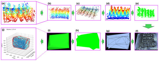
Figure 9.
Point cloud data processing for plant height and canopy volume estimation. (a) PCD (point cloud) map; (b) segmentation of region of interest (ROI) of six rows; (c) downsampling; (d) filtering for denoising and outlier removal; (e) inlier separation; (f) preparing the canopy mesh; (g) making convex hull mesh; (h) unsmooth convex hull; (i) smooth convex hull for calculating the volume of convex hull; (j) sensor estimated canopy volume.
2.4.2. Plant Spacing and Row Distance
Raw LiDAR data (pcap format) were converted to PCD files and parsed into three-dimensional (x, y, z) coordinates. The data underwent multiple processing steps such as filtering and outlier removal to eliminate noise, downsampling to reduce point density, and segmentation to isolate the plant rows of interest. Clustering algorithms grouped points into distinct rows or plant clusters, and the centroids of the clusters were calculated to enable center-to-center distance measurements between consecutive points. Figure 10 provides a visual context comprising the LiDAR sensor setup in the field, a color-coded point cloud, and the final processed point cloud with clearly delineated rows for precise calculation of row spacing and plant distance. The integrated approach yielded quantitative metrics crucial for agronomic decision-making, including characterization of planting uniformity and canopy structure in the real field.
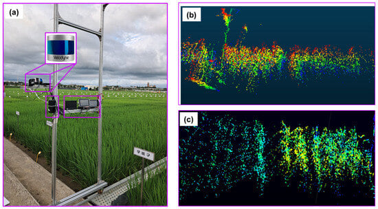
Figure 10.
Visualization of the rice canopy for estimating the row distances and plant spacing. (a) data acquisition for row distance and plant spacing measurement; (b) visualization of point cloud data and the PCD map; (c) visualization of point clouds of six rows of rice plants segmented from a selected data frame for row distance and plant spacing measurement.
Python was used as the primary framework for data handling and analysis, enabling the conversion of raw LiDAR data (pcap format data) into a workable point cloud format (PCD). Subsequent filtering and outlier removal processes, as shown in Figure 10, ensured that only high-quality points remained. Python libraries such as Open3D (version 0.18.0) or NumPy (version 1.24.3) were used for processing. The point cloud was then segmented and clustered into individual plant rows, enabling centroid calculations for each cluster. This approach facilitated accurate row-to-row distance measurements. Furthermore, plant spacing within each row was determined by identifying and measuring the distance between consecutive plant clusters. This Python-oriented workflow provided a robust and flexible platform for automating data preprocessing, segmentation, and distance calculation, ultimately offering reliable metrics for evaluating planting uniformity (plant spacing and row distance) and canopy structure. The raw LiDAR point cloud was initially loaded and subjected to outlier removal (via radius-based filtering) and voxel downsampling, minimizing noise and reducing data density while storing geometric plant features. After that, the ground segmentation using the random sample consensus (RANSAC) plane fitting algorithm isolated the canopy or plant rows, where any remaining irrelevant data points were excluded. Depending on whether row distance (Y-axis) and plant (hill-to-hill) spacing (X-axis) were in the ROI, the algorithm sorted the remaining points along the relevant axis. Using prior knowledge of the experimental layout, such as the total width (or length) occupied by a fixed number of rows, including the number of gaps between them, the average plant spacing was calculated as the total estimated dimension divided by the number of gaps plus one. This approach might be refined with clustering algorithms such as density-based spatial clustering of applications with noise (DBSCAN) algorithm to distinguish individual plant clusters. The result was a robust, semi-automated pipeline in Python that integrated data denoising, ground plane removal, coordinate-based filtering, and geometric calculations of row distance and plant spacing.
2.5. Statistical and Analytical Procedures
The geometric features, including tree height, canopy volume, row distance, and plant spacing, were compared between manual measurement and LiDAR measurement data through linear regression analysis. For better demonstration and understanding of the estimation of geometric features of rice plants, the mean error calculation was performed. The mean error in rice plant feature estimation better reflected the accuracy of the estimation method and accounted for the variability between individual plants of different heights, canopy volumes, plant spacing, and row distance. To assess the accuracy of the developed data processing algorithm, the coefficient of determination (r2), root mean squared error (RMSE), mean absolute error (MAE), bias (mean difference), confidence interval (CI) with 95% confidence for the mean difference, standard deviation (), and t-test statistic, and accuracy (%) were calculated using Equations (2)–(9), respectively, as follows [,]:
where and are the measured and sensor-estimated values, respectively, and is the average of the sensor estimated values. and are the sensor-estimated values for observations. n is the number of observations. Bias indicates whether the sensor estimated values consistently overestimated (>0) or underestimated (<0) the manual measurement values. is the mean difference (bias). indicates standard deviation of the differences , and is the critical value of t-distribution with degrees of freedom at the desired confidence level (95%).
Equation (9) determined how closely the LiDAR measurement results were aligned with the measure results or ground truth measurements, where higher accuracy (%) indicated better agreement and lower accuracy (%) indicated deviations during the measurements of vegetative growth monitoring parameters due to factors like vegetation density and occlusion.
3. Results
3.1. Geometric Characteristics at Three Growth Stages
Table 2 compares key statistical parameters (mean, standard deviation, RMSE, r2, MAE, Bias, t-statistic, p-value, and 95% CI) for plant height, canopy volume, row distance, and plant spacing during the early, middle, and late growth stages. The Phase comparison column highlights the trend of each parameter across the phases.

Table 2.
Statistical summary of LiDAR and manual measurements of rice plant geometric characteristics across growth phases.
3.1.1. Geometric Characterization in Early Growth Stage
Table 2 presents a statistical summary of LiDAR and manual measurements for plant height, canopy volume, row distance, and plant spacing in the early, middle, and late growth stages. Table 2 shows that in the early growth stage, LiDAR measurement and manual measurement height were 0.5 ± 0.06 m and 0.48 ± 0.03 m, respectively. The mean values for plant height estimation showed a small overestimation of 0.02 ± 0.03 m by LiDAR measurement than manual measurement values. The RMSE was 0.04, and the r2 value of 0.96 indicated a strong correlation and measurement deviation between LiDAR measurement and manual measurement results. The r2 value of 0.96 showed a 96% correlation between LiDAR measurement and manual measurement height, indicating the high accuracy of LiDAR in estimating plant height. The MAE of 0.022 m and bias of 0.003 m indicated that LiDAR overestimated plant height by 0.003 m (0.62%) compared to manual measurement results. The t-statistic value of 0.331 and p-value of 0.745 indicated that there was no statistically significant difference between LiDAR measurement and manual measurement height. Moreover, the 95% CI (−0.016, 0.022) supported that the variation in plant height estimation was small and within an acceptable range, whereas LiDAR provided closely accurate plant height measurements with a low value of bias and a strong correlation.
Canopy volume measurement using LiDAR and the manual measurement volume were 0.7 ± 0.05 m3 and 0.69 ± 0.04 m3, respectively, which indicated that LiDAR overestimated the canopy volume by a small value of 0.01 ± 0.01. The RMSE was 0.04, which further supported the deviation, and the r2 value of 0.95 showed a strong correlation. The MAE of 0.037 m3 and bias of −0.027 m3 indicated that LiDAR underestimated canopy volume by 0.027 m3, which was approximately 3.91% compared to the measured canopy volume. The t-statistic value of −3.031 and p-value of 0.007 indicated a statistically significant difference between LiDAR measurement and manual measurement canopy volume. The 95% CI (−0.045, −0.008) indicated that LiDAR underestimated the canopy volume by a range of 1.16% to 6.52% compared to the measured volume. The negative values confirm an underestimation of canopy volume between 0.008 m3 and 0.045 m3, indicating that LiDAR measurement canopy volumes were lower than the measured canopy volume.
During row distance measurement, LiDAR and manual measurement distance were 0.3 m and 0.3 ± 0.01 m, respectively, which indicated that LiDAR was highly accurate in measuring row distances in the early growth stage of rice. RMSE was very low (0.01), and r2 was 0.98, indicating a very strong correlation. The MAE of 0.007 m and bias of 0.0001 m confirmed a measurement error of 0.70% and a bias of 0.03% compared to the manual measurement of row distance. The small bias value indicated that LiDAR measurement results for row distance were highly accurate, with only a 0.0001 m deviation from manual measurement results. The t-statistic value of 0.041 and p-value of 0.968 indicated that the difference was not statistically significant. The 95% CI values (−0.005, 0.005) indicated a measurement variation of approximately 1.67% compared to the measured row distance. This confirmed that the difference between LiDAR measurement and manual measurement row distance was only 0.005 m, highlighting the statistical insignificance of the difference (p-value = 0.968).
LiDAR measurement of plant spacing and manual measurement spacing were 0.2 ± 0.001 m and 0.2 ± 0.01 m, respectively, which indicated that LiDAR performed well in plant spacing measurements. RMSE had a low value of 0.01, and r2 had a value of 0.96, showing a strong correlation between LiDAR estimated and measured results. The MAE of 0.007 m and bias of 0.002 m indicated a measurement error of 3.5% and an overestimation of 1% compared to the measured results. This confirmed that LiDAR measurement of plant spacing differed by 0.002 m with respect to the manual measurement of plant spacing. The 95% CI of −0.002, and 0.007 confirmed that plant spacing deviations range from approximately 1% to 3.50% compared to manual measurement of plant spacing. It indicated that LiDAR measurement of plant spacings were consistent with manual of measurement of plant spacing, with deviations limited to a maximum of 3.50%. LiDAR provided accurate plant spacing measurements, with low errors, and a non-significant difference was found in measured results.
The variability between LiDAR measurement results and manual measurement results are visualized in Figure 11a–d, where blue bars show the manual measurement results and orange indicates the LiDAR measurement results of 20 selected data samples. The orange and blue dotted lines indicate the average values of LiDAR measurement and manual measurement results, respectively, for each vegetative growth monitoring parameter in the early growth stage of rice.
3.1.2. Plant Characteristics Measurement in Middle Growth Stage
In the middle growth stage, LiDAR measurement of plant height and manual measurement of height were found to be the value of 0.93 ± 0.13 m and 0.92 ± 0.04 m, respectively, which indicated an overestimation of 0.01 ± 0.09 m (1.09%) by LiDAR. The RMSE was 0.06 m, indicating a measurement deviation of 6.52%. The r2 value of 0.96 confirmed a 96% correlation, demonstrating a strong agreement between LiDAR measurement and manual measurement results. The MAE was 0.0295 m (3.21%), while the bias was −0.0125 m (−1.36%), indicating a small but consistent underestimation. The t-statistic value of −1.5004 and p-value of 0.1499 suggested that there was a statistically non-significant difference in height measurements. The 95% CI of (−0.0299, 0.0049) demonstrated that variations in plant height estimations ranged from −3.25% to 0.53%.
During canopy volume measurements, LiDAR measurement and manual measurement volumes were 1.3 ± 0.12 m3 and 1.33 ± 0.1 m3, respectively, which indicated that LiDAR underestimated canopy volume by 0.03 m3 (2.26%). The RMSE was 0.05 m3, exhibiting an error of 3.76%. Moreover, the r2 value of 0.97 indicated a 97% correlation, showing a strong relationship between LiDAR measurement and manual measurement results. The MAE was 0.0375 m3 (2.82%), and the bias was −0.0205 m3 (−1.54%). This confirmed that LiDAR underestimated canopy volume by 0.0205 m3, which corresponded to 1.54% compared to manual measurement results. This underestimation indicated that LiDAR measurement of canopy volume was lower than manual measurement values, with a deviation of up to 2.82% in absolute error. The t-statistic of −1.9858 and p-value of 0.0617 indicated that the difference was not statistically significant. The 95% CI (−0.0421, 0.0011) indicated a possible underestimation ranging from −3.17% to 0.08%.
LiDAR measurement of row distance and manual measurement of distance were 0.38 ± 0.02 m and 0.40 ± 0.02 m, respectively, showing a significant underestimation of 0.08 m (20%) by LiDAR, whereas the RMSE value was 0.02 m. The RMSE indicated a measurement deviation of 5%. The r2 value was found to be 0.94, which suggested a 94% correlation, showing a strong relationship. The MAE of 0.0230 m (5.75%) and the bias of −0.0230 m (−5.75%) confirmed a consistent underestimation of 5.75% by LiDAR for row distance measurements compared to manual measurement results. Furthermore, the t-statistic of −18.0063 and p-value of 0 confirmed a statistically significant difference between LiDAR measurement and manual measurement results. Additionally, the 95% CI (−0.0257, −0.0203) showed that LiDAR significantly underestimated row distance, with deviations ranging from 5.08% to 6.43%, and the difference was statistically significant in the middle growth stage of rice.
For plant spacing measurement, LiDAR estimated spacing and manual measurement spacing were 0.19 ± 0.01 m and 0.20 ± 0.01 m, respectively, which showed an underestimation of 0.01 m (5%) by LiDAR. The RMSE value was 0.01 m, indicating a measurement deviation of 5%. The r2 value was found to be 0.94, indicating a 94% correlation, which showed a strong relationship. The MAE of 0.011 m (5.5%) and the bias of −0.006 m (−3%) confirmed an underestimation of 3% in LiDAR measurement results for plant spacing measurements compared to manual measurement results. This indicated that LiDAR measurement of plant spacing was 0.006 m lower than the manual measurement results, with an absolute deviation of up to 5.5%. This suggested that LiDAR measurement of plant spacing deviated 5.5% from the manual measurement results.
Figure 12a–d demonstrate the variability between LiDAR estimated results and the manual measurement results, where blue bars show the manual measurement results and orange indicates the LiDAR measurement results of 20 selected data samples. The orange and blue dotted lines indicate the average values of LiDAR measurement and manual measurement results, respectively, for each vegetative growth monitoring parameter in the middle growth stage of rice.
3.1.3. Measurement of Rice Plant Characteristics in Late Growth Stage
In the late growth stage, LiDAR measurement of plant height and manual measurement height were found to have values of 0.99 ± 0.06 m and 1.02 ± 0.04 m, respectively, which showed an underestimation of 0.03 m (2.94%) by LiDAR. The RMSE value was 0.04 m, which showed a measurement deviation of 3.92%. The r2 value was found to be 0.97, which confirmed a 97% correlation, demonstrating a strong agreement between LiDAR measurement and manual measurement results. The MAE was 0.03 m (2.94%), while the bias was −0.02 m (−1.96%), confirming a consistent underestimation of 1.96% by LiDAR for plant height measurements compared to manual measurement results. It also indicated that LiDAR measurement of the plant height was 0.02 m lower than manual measurement results, with an absolute deviation of up to 2.94%. The t-statistic of −3.17 and p-value of 0.01 indicated a statistically significant difference in height measurements. Furthermore, the 95% CI of −0.04, and −0.01 confirmed that variations in plant height estimations ranged from −3.92% to −0.98%.
LiDAR estimated row distance and manual measurement distance were 0.38 ± 0.03 m and 0.39 ± 0.02 m, respectively, which showed an underestimation of 0.01 ± 0.01 m (2.56%) by LiDAR. The RMSE was 0.03 m, indicating a measurement deviation of 7.69%. The r2 value obtained of 0.94, which showed a correlation of 94%, and exhibited a strong relationship between LiDAR measurement and manual measurement results. The MAE was 0.02 m (5.13%), and the bias was −0.01 m (−2.56%), which also confirmed an underestimation. The t-statistic of −3.01 and p-value of 0.01 also confirmed that the difference was statistically significant. The 95% CI (−0.02, −0) indicated an underestimation ranging from −5.13% to −0%, and the difference was statistically significant.
During row distance measurement, LiDAR-estimated distance and manual measurement distance were 0.38 ± 0.03 m and 0.39 ± 0.02 m, respectively, which showed an underestimation of 0.01 ± 0.01 m (2.56%) by LiDAR. The RMSE was 0.03 m, indicating a measurement deviation of 7.69%. The r2 value obtained was 0.94, which showed a correlation of 94%, exhibiting a strong relationship between LiDAR measurement and manual measurement results. The MAE was 0.02 m (5.13%), and the bias was −0.01 m (−2.56%), which also confirmed an underestimation. The t-statistic of −3.01 and p-value of 0.01 also confirmed that the difference was statistically significant. The 95% CI (−0.02, −0) indicated an underestimation ranging from −5.13% to −0%, and the difference was statistically significant.
LiDAR-estimated plant spacing and manual measurement of spacing were of 0.18 ± 0.01 m and 0.20 ± 0.01 m, respectively, showing an underestimation of 0.02 m (10%) by LiDAR. RMSE value was 0.02 m, which also indicated a measurement deviation of 10%. The r2 value of 0.88 showed 88% correlation, which indicated a strong relationship. The MAE was 0.02 m (10%), and the bias was −0.02 m (−10%), confirming a consistent underestimation. The t-statistic of −9.98 and p-value of 0 confirm that the difference was statistically significant. The 95% CI (−0.03, −0.02) indicated an underestimation ranging from −15% to −10%. Figure 13a–d demonstrate the variability between LiDAR measurement results and the manual measurement results, where blue bars show the manual measurement results and orange indicates the LiDAR measurement results of 20 selected data samples. The orange and blue dotted lines indicate the average values of LiDAR measurement and manual measurement results, respectively, for each vegetative growth monitoring parameter in the middle growth stage of rice.
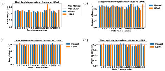
Figure 11.
Visualization of LiDAR measurement and manual measurement results for measuring the vegetative growth monitoring parameters in the early growth stage of rice (23 days after transplanting). (a) Plant height (m); (b) canopy volume (m3); (c) row distance (m); and (d) plant spacing (m). Orange and blue dotted lines indicate the level of mean values of LiDAR measurement and manual measurement results, respectively. Orange and blue bars indicate the LiDAR measurement and manual measurement results, respectively.
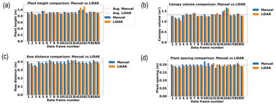
Figure 12.
Measurement and comparison of plant geometric features in the middle growth stage of rice (53 days after transplanting). (a) Plant height (m); (b) canopy volume (m3); (c) row distance (m); and (d) plant spacing (m).
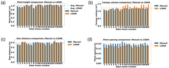
Figure 13.
Measurement and comparison of plant geometric features in the late growth stage of rice (80 days after transplanting). (a) Plant height (m); (b) canopy volume (m3); (c) row distance (m); and (d) plant spacing (m).
3.2. LiDAR Measurement Accuracy Across Growth Monitoring Parameters
Figure 14a illustrates the accuracy (%) of vegetative growth monitoring parameters in the early growth stage of rice. In the early growth stage, an accuracy of 95–97% was found across the vegetative growth monitoring parameters, indicating the reliability of LiDAR measurement results. Plant height, with a measurement accuracy of 95.58% and plant spacing measurement accuracy of 96.43%, exhibits strong reliability, indicating that LiDAR can accurately measure individual plant geometric features such as plant height and plant spacing in an early growth stage. Figure 15a also demonstrates the canopy volume accuracy of 94.72%, whereas row distance has the highest accuracy at 97.70%, indicating that row separations were detectable in the early stage due to sparse canopy interference.
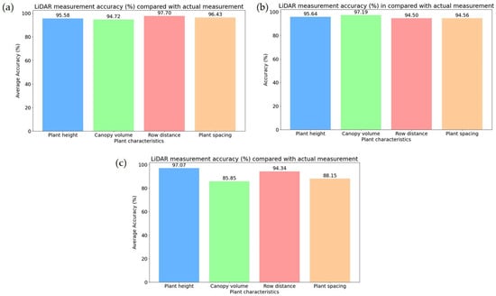
Figure 14.
Comparison of accuracy between LiDAR and manual measurement results of estimating the plant geometric features in the different growth stages of rice. (a) Early growth stage; (b) middle growth stage; (c) late growth stage.
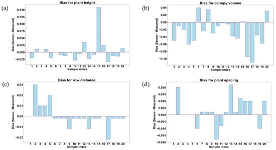
Figure 15.
Comparison and measurement of bias for rice plant geometric features in the early growth stage of rice. (a) plant height (m); (b) canopy volume (m3); (c) row distance (m); and (d) plant spacing (m).
The accuracy (%) of measuring the vegetative growth monitoring parameters in the middle growth stage is shown in Figure 14b. Plant height measurement accuracy was found to have a value of 95.64%, whereas row distance accuracy was found to be the value of 94.50%, indicating LiDAR measurement results remain reliable for the growth of vegetative growth monitoring. Canopy volume estimation showed the highest accuracy of 97.19%, suggesting that LiDAR performed volume estimations well in the middle growth stage due to dense canopy structures. Conversely, plant spacing measurement accuracy was found to be the value of 94.56%, remaining lower than the early stage (96.43%), which could be due to denser foliage affecting individual plant detection.
Figure 14c exhibits the vegetative growth monitoring parameters in the late growth stage, where a decline in accuracy (%) was observed for most of the parameters compared to the early growth stage, indicating that dense canopy structures in the late growth stage affect the LiDAR performance. The highest accuracy of 97% was found during the measurement of plant height, which showed that LiDAR was highly effective for height estimation despite increased canopy complexity. It was also exhibited that row distance accuracy was reduced to 94.34%, likely due to occlusion effects from overlapping leaves. Plant spacing accuracy was also reduced to 88.15%, indicating that LiDAR struggled with detecting individual plants due to the growth density of plants. Canopy volume accuracy experienced the most significant decline in accuracy of 85.85%, indicating challenges in precisely estimating volume due to increased vegetation density and occlusion effects in the late growth stage of plants.
Figure 15a,b illustrate the deviations between the LiDAR measurement and manual measurement results for rice plant geometric features such as plant height, canopy volume, row distance, and plant spacing at 23 days after transplanting. In Figure 15a,b, each bar represents a sample index, with positive values indicating LiDAR overestimation and negative values indicating LiDAR underestimation compared to manual measurements. Figure 15a shows that in measurements for plant height, most of the samples (12 samples out of 20) exhibit a bias close to the value of zero, which indicates a high agreement between LiDAR measurement and manual measurement of plant heights. Some of the samples (5 samples out of 20) showed slight underestimation (0.02–0.035 m), while a few (3 samples out of 20) showed overestimated heights (0–0.165 m), particularly in sample number 15, where the highest positive bias value of 0.165 m was obtained among 20 data samples. In Figure 16a, small differences suggest that LiDAR was highly reliable for height estimation, though irregular overestimation might be found due to irregular leaf structure or noise as well as the complex geometry of plants. Figure 15b shows that the canopy volume bias varied significantly across samples, with both overestimation (positive value) and underestimation (negative value). Most of the samples (12 samples out of 20) showed negative bias (>−0.11 m3), which indicated an underestimation in LiDAR measurement of rice canopy volume. Among 20 data samples (data frames), 3 samples showed an overestimation of bias that indicated a positive bias, while 5 samples indicated a bias close to the value of 0 m3. These variations in bias were due to the complex geometry of plants, leaf angles, or occlusion effects affecting the ability of LiDAR to capture whole canopy volume.
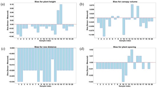
Figure 16.
Comparison and measurement of bias for rice plant geometric features in the middle growth stage of rice. (a) Plant height (m); (b) canopy volume (m3); (c) row distance (m); and (d) plant spacing (m).
In Figure 15c, a positive bias was found in some samples (4 samples out of 20) during the measurements of row distance bias, while a negative bias was found in other samples (14 samples out of 20). Among the 14 samples out of 20 that showed negative bias, only 3 samples showed bias values of −0.01 to −0.02 m, and the remaining 12 samples out of these 14 samples showed bias values close to zero, where only 2 samples (sample index 1 and 16) showed a bias value of 0 m. Samples 2–5 exhibit overestimation, while samples 9, 13, and 17 showed moderate to high bias values, as well as indicating underestimation. The underestimation trend indicates that LiDAR struggles to detect row separations accurately due to overlapping leaves or limitations in distinguishing gaps between rows for precise row distance measurement. These results suggest that LiDAR may require improved angle positioning or multi-view scanning to enhance row distance detection accuracy. Figure 16d demonstrates that the bias for plant spacing fluctuated, with 2 samples out of 20 (sample indices 2 and 13) showing an overestimation of around 0.02 m. Among the 20 data samples, 4 samples (samples index 6, 10, 11, and 19) displayed underestimation ranges from −0.07 to −0.02 m. Moreover, the negative bias in certain samples indicated that LiDAR underestimates plant spacing, potentially due to the variation in the density of vegetation of individual plants. The variability also indicates that plant spacing measurements are affected by plant positioning, sensor angle, and LiDAR beam penetration. At 23 days after transplanting, LiDAR demonstrated strong accuracy for plant height measurements, while canopy volume, row distance, and plant spacing exhibited underestimation and overestimation in plant geometric feature monitoring during the early growth stages of rice.
Figure 16a,b illustrate the deviations between LiDAR measurement and manual measurement results for geometric features such as plant height, canopy volume, row distance, and plant spacing of rice plants at the middle growth stage (53 days after transplanting). The bias is calculated as the difference between LiDAR measurement and manual measurement values during the measurements of geometric features of rice plants. This indicated an overestimation when a positive bias value was observed and an underestimation when a negative bias value was observed during the measurements. The trends in these graphs provide insights into the accuracy of LiDAR measurement and manual measurement differences with plant growth progress. Figure 16a shows the bias values that were obtained during the measurement of plant height. Most of the samples showed a negative bias, indicating that LiDAR underestimated plant height compared to manual measurement results. A few samples, such as data samples 15 and 16, exhibited strong overestimations of 0.07 and 0.10 m, respectively, which could be due to outliers in LiDAR measurement results or incorrect plant edge detection. In the middle growth stage, 17 data samples out of 20 showed underestimation in LiDAR measurement results compared with manual measurement results, while only data sample 5 showed a 0 m bias. The overall underestimation trend might be due to increased leaf bending and overlapping foliage, causing LiDAR to detect lower points instead of actual plant tips. Figure 16b shows the bias during the measurement of plant canopy volume of rice plants in the middle growth stage. The bias distribution was found to be highly variable (−0.11 m3 to 0.08 m3), with samples 13 and 15 showing overestimation of 0.08 m3 and 0.07 m3, respectively. Other samples, except sample 9 (bias value of 0 m3) among 20 data samples, indicated underestimation (up to −0.11 m3). The large fluctuations of bias values also indicate that the accuracy of LiDAR measurement results might decline with plant density increases during the measurement of canopy volume. The underestimation trend in multiple samples indicated that LiDAR was struggling to capture full canopy volume due to overlapping leaves and occlusion effects.
In Figure 16c, almost all samples showed negative bias, with values reaching −0.03 m, indicating that LiDAR consistently underestimated row distance in the middle growth stage. This underestimation was likely caused by dense foliage and canopy closure, which made it difficult for LiDAR to detect rows accurately with separations between each other. This pattern also suggested that as rice plants grew, row detection became increasingly challenging due to occlusion effects. Similarly, in Figure 16d, most of the samples, except 5 samples out of 20, show a negative bias (up to −0.03 m), confirming that LiDAR underestimated plant spacing in the middle growth stage. Only 4 samples out of 20 showed an overestimation of bias values up to 0.02 m, whereas only 1 sample showed 0 m of bias. The significant underestimation trend highlighted the difficulty of LiDAR in distinguishing individual plants when canopy coverage was increased.
Deviations between LiDAR-estimated and manual measurement results for geometric features of rice plants at the late growth stage (80 days after transplanting) are illustrated in Figure 17a,b. These trends also provided insights into how the accuracy was affected by increasing canopy density and plant structural complexity of rice during the vegetative growth monitoring using the proximal LiDAR sensing technique in the late growth stage. In Figure 17a, most of the samples (15 samples out of 20) show negative bias (from −0.01 to −0.08 m), indicating that LiDAR underestimated plant height in comparison with manual measurement results. Four samples out of twenty (samples 7, 10, 11, and 15) showed positive bias (0.01 to 0.03 m), indicating overestimation due to outliers or noise in LiDAR measurement results. The underestimation trend became more pronounced compared to early growth stages, likely due to increased leaf bending and occlusion effects in dense canopies. Figure 17b shows large variations in bias values during canopy volume measurement, with positive bias up to 0.27 m3 and negative bias up to −0.16 m3. The overestimation trend dominated in late growth stages, possibly due to LiDAR measurement results and the overlapping of the canopy. Conversely, the underestimation in certain samples indicated that some dense canopy regions might have still obstructed the LiDAR scans, reducing the detected volume. In Figure 17c, most of the samples (14 samples out of 20) show negative bias (−0.01 to −0.05 m), confirming that LiDAR significantly underestimated the row distance in the late growth stage. Only three samples (samples 3, 4, and 17) exhibited a positive bias of 0.02 m, indicating overestimation in sparse areas. The consistent underestimation trend suggested that row distance measurements became more challenging with increasing plant density, further occluding row distances. Moreover, the bias was consistently negative (−0.01 to −0.04 m) across all samples, as shown in Figure 17d, meaning LiDAR continuously underestimated the plant spacing in the late growth stage.
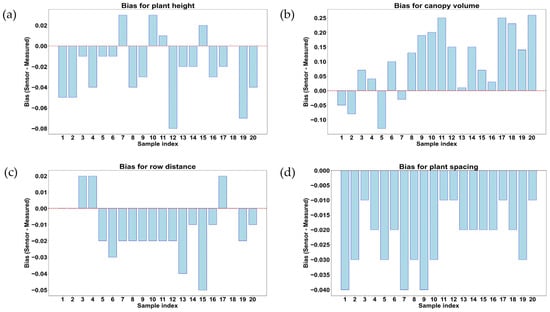
Figure 17.
Comparison and measurement of bias for rice plant geometric features in the late growth stage of rice. (a) Plant height (m); (b) canopy volume (m3); (c) row distance (m); and (d) plant spacing (m).
4. Discussion
This study introduces a customized point cloud processing algorithm integrating frame screening, outlier removal, denoising, voxelization, and geometric feature extraction designed specifically for accurate and efficient rice canopy characterization across growth stages, setting it apart from standard LiDAR processing approaches. Due to the complex plant geometry of rice, accurately measuring vegetative growth parameters has long been challenging, often requiring specialized instruments like those for projected leaf area. LiDAR effectively captures vertical structural features, enabling detailed reconstruction of plant geometry. In this study, a rice-specific geometric feature extraction algorithm was developed that efficiently acquired high-resolution point cloud data, including features that are difficult to measure with traditional methods. Plant geometric features such as plant height, canopy volume, row distance, and plant spacing were extracted across three different growth stages, demonstrating strong correlation and high reliability []. The performance of LiDAR sensing for precise plant height measurement is also proved by numerous studies; for example, a commercial LiDAR was used for plant height estimation and showed that the number of laser pulses reaching the ground surface decreases as rice growth progressed. Their study also mentioned that since paddy fields are typically filled with water, laser pulses often struggle to reach the ground surface, as certain laser wavelengths tend to be fully or partially absorbed by water with more than 4 cm of clear water depth []. Furthermore, it also demonstrated that due to the vegetation coverage being 20%, more than 50% of laser pulses cannot reach the ground surface and are absorbed by the water. This is one of the reasons behind the error of plant height estimation in early growth stages of rice. Since, in this critical stage, most of the time there was standing water, as it is an early vegetative growth stage, LiDAR measurement may struggle with this limitation. In this study, there was also standing water with around 4–5 cm water depth during the data acquisition, which might have some effects on height measurement. Rice plant height was estimated using LiDAR measurement and reported estimation errors of 14, nearly 10, and 5 cm, respectively [,,], whereas the error of 2–3 cm was obtained during the measurement of LiDAR measurement of plant height in this study.
Figure 18 effectively illustrates the dynamics of rice plant growth and highlights the differences between the growth stages. Figure 18a,b represent the growth curves of rice plant height and canopy volume, respectively, across the early, middle, and late growth stages, comparing LiDAR measurements with manual measurements. Both parameters showed a consistent upward trend from the early to the middle stage, followed by a slight decline at the late stage. The LiDAR and manual measurements exhibited similar patterns, indicating strong agreement. However, manual measurements tended to slightly overestimate plant height in the late stage, while LiDAR consistently reported higher canopy volume. These results demonstrated that LiDAR sensing is a reliable, nondestructive alternative for monitoring rice growth dynamics with comparable accuracy to manual methods.
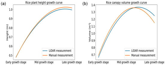
Figure 18.
Visual representations of rice plants using growth curves to illustrate changes across the early, middle, and late growth stages. (a) Plant height (m); (b) canopy volume (m3).
However, canopy volume estimation needs further refinement, as LiDAR tends to slightly underestimate the actual volume. Future improvements, such as multi-angle LiDAR scanning or sensor adjustments, could enhance accuracy, particularly for canopy structure estimations. Jing et al. [] investigated the use of LiDAR for estimating rice canopy height, emphasizing the necessity of accurate ground elevation data for precise measurements where LiDAR was fixed above the canopy, maintaining a consistent nominal distance from the ground in that study. It also supports the LiDAR setup with the data acquisition structure, which was followed in this study during the data acquisition in the rice field. In this study, the results exhibited that during the early growth stage, LiDAR measurement results closely matched the manual measurements, with accuracy ranging from 95% to 98% across the vegetative growth monitoring parameters of rice, such as plant height, canopy volume, row distance, and plant spacing. In the middle growth stage, the errors increased in canopy volume and row distance measurement due to greater plant density and occlusion effects. By the late growth stage, accuracy declined to 85.85% for canopy volume, 94.34% for row distance, and 88.15% for plant spacing, as the denser canopy limited the ability of LiDAR to capture precise measurements. This finding is also supported by the findings of the study by Jing et al. []; for example, when rice plant density increased to later growth stages, it significantly limited laser beam penetration, causing most LiDAR points to originate from the canopy top rather than the ground. The study also mentioned that height accuracy was affected even in a smaller area (12 × 6 m), with errors ranging from 0.24% to 12.98%.
Sensitivity analysis in this study confirmed that LiDAR underestimation increased gradually with growth stage advancement, particularly for canopy volume and plant spacing. The bias analysis further revealed that measurement discrepancies became more pronounced in the middle and late growth stages, indicating a decline in the effectiveness of LiDAR, particularly in measuring plant spacing and row distance, as plant density increases. In this study, variation was found between manual measurement results and the LiDAR measurement results, which is clarified by the underestimation and overestimation of the parameters between manual measurement and sensor-estimated results. This is also supported by a study that indicated that LiDAR is more accurate than manual inspection [].
LiDAR has growing practical significance in precision agriculture. As highlighted in recent reviews, LiDAR supports a wide range of agricultural applications from crop growth estimation and disease detection to weed control and plant health evaluation. In the context of rice production, high-resolution LiDAR data can aid plant breeding programs by enabling the selection of desirable traits such as canopy architecture and plant spacing, which influence light interception and yield []. This study may also contribute to serving these purposes for rice cultivation. For real-time growth monitoring, LiDAR allows non-destructive, repeatable measurements that help track vegetative development and detect stress conditions, which is another practical application of LiDAR aligned with this study. This study’s results can play a vital role in providing an inexpensive way of enhancing site-specific monitoring of rice, which is supported by the study’s findings of crop monitoring in agriculture [,,].
Moreover, LiDAR measurements are valuable in site-specific fertilizer and pesticide applications for judicial use of agricultural inputs such as pesticide and fertilizers, which will assist in improving efficiency and reducing the environmental impact. As a part of the practical application of this study, in fertilizer and pesticide application planning, the measurement results obtained from LiDAR measurement can help identify areas of uneven canopy growth or plant density, allowing for targeted input application, which may enhance resource efficiency and reduce the environmental impact []. Based on these measurements, LiDAR may be integrated into automated crop modeling systems and may also enhance predictions of crop growth and yield under varying field conditions. These will not only contribute as a critical tool to phenotyping but also to broader agronomic decision-making. It might be supported by its expanding use in precision agriculture platforms, including autonomous field systems for rice cultivation. This technique may also be used for the growth monitoring of other similar types of crops (e.g., wheat, maize, pulse and oilseed crops, etc.), which may help in pruning/thinning, spraying, and other intercultural operations [].
However, the use of LiDAR in agriculture, particularly in rice fields, presents several challenges. Despite being a powerful sensor for non-contact growth monitoring, LiDAR-estimated feature characterization faced challenges, particularly in the late growth stages of rice due to canopy occlusion, measurement biases, and sensor positioning limitations, when dense rice canopies may block LiDAR scans. Among the challenging issues, canopy occlusion and leaf overlapping were major issues, which obstructed LiDAR beams and led to the underestimation of plant spacing and row distance, especially in the middle to late growth stages []. Similarly, plant height measurements could be underestimated due to leaf bending, while canopy volume fluctuated between overestimation (due to multiple reflections from overlapping leaves) and underestimation (caused by occluded lower canopy layers). This occlusion results in incomplete point cloud data, which can reduce the accuracy of measurements. Environmental factors such as wind-induced plant movement and ground reflection effects introduced additional variability, particularly in early growth stages, when the canopy was sparse. Furthermore, preprocessing of LiDAR-scanned point clouds requires computational power, such as filtering, noise, segmenting plant features, and correcting measurement errors, which demand advanced algorithms. The recorded measurements were used for additional analysis based on visual estimations in this study, which was not formally recorded regarding the observer bias during the visual estimation process. Due to the subjective nature of visual estimations, some levels of bias may have been introduced that were unable to quantify or measure the bias due to the lack of recorded observations. Consequently, it was unable to provide a specific error estimate, which was one of the limitations of the study. Therefore, it was recommended that future work could benefit from a more structured approach, including recording observations and assessing potential bias, to better understand an account for the estimation errors.
Future Research Directions and Limitations
While LiDAR is an effective tool for monitoring rice plant growth, there are still some limitations, particularly related to canopy occlusion. As rice plants grow, their dense canopies can obstruct LiDAR scans, leading to incomplete data in the later growth stages. The challenges, including water reflection and variable plant architecture, reduce the LiDAR measurement accuracy, which was also a challenge in this study, especially in the middle to late growth stages. To overcome this challenge, future research could explore the integration of complementary sensors, such as multispectral cameras or hyperspectral sensors, which might provide additional data to fill in gaps caused by canopy occlusion. Future research should explore integrating LiDAR with other sensing techniques (e.g., remote sensing using RGB, ultrasonic, depth camera, and multispectral camera), using multi-angle scanning setups, and improving point cloud filtering and occlusion correction algorithms.
Additionally, refining the ground-point removal algorithms and canopy height extraction methods could further improve the precision of LiDAR measurements, particularly for dense rice canopies. Future studies should also explore automatic algorithms for volume estimation and investigate ways to reduce the computational load while maintaining high data resolution.
Therefore, adapting LiDAR systems to various rice cultivation practices and working environments may further enhance the application of LiDAR in smart farming systems, particularly in the cultivation of rice.
5. Conclusions
This study evaluated the performance of LiDAR in estimating rice plant geometric features for vegetative growth monitoring across three different growth stages, namely the early, middle, and late growth stages. The LiDAR-estimated results of plant height, canopy volume, row distance, and plant spacing measurement were compared with manual measurement results using statistical metrics such as RMSE, r2, MAE, bias, t-statistic, p-value, and 95% CI. The results demonstrated that LiDAR estimated the plant height accurately across the three growth stages, with a strong correlation (r2 > 0.95) and a minimal measurement bias ranging from −0.02 m to 0.003 m. However, canopy volume, row distance, and plant spacing estimations exhibited deviation depending on the growth stage. The canopy volume showed an underestimation of up to −0.11 m3 in the early growth stage and −0.112 m3 in the middle growth stage and an overestimation of up to 0.25 m3 in the late growth stage. The row distance estimation exhibited an underestimation of up to −0.025 m in the early growth stage, −0.030 m in the middle growth stage, and −0.05 m in the late stage. Plant spacing estimation showed an underestimation of up to −0.018 m in the early growth stage, −0.03 m in the middle growth stage, and −0.040 m in the late stage.
In the early growth stage, LiDAR estimated results closely reached the manual measurements, with accuracy around 95% to 98% for all parameters. The middle growth stage showed slightly increased errors in canopy volume and row distance, primarily due to increased plant density and occlusion effects. In the late growth stage, accuracy declined for canopy volume (85.85%), row distance (94.34%), and plant spacing (88.15%) as dense canopy structures interfered with the ability of LiDAR to capture precise measurements. Sensitivity analysis confirmed that LiDAR underestimation increased gradually with growth stage advancement, particularly for canopy volume and plant spacing. Bias analysis further revealed that measurement discrepancies became more pronounced in the middle and late growth stages, indicating a decline in the effectiveness of LiDAR, particularly in measuring plant spacing and row distance, as plant density increases. The study confirms that LiDAR is a reliable tool for monitoring plant height and canopy volume in the early and middle growth stages. However, as canopy complexity increases, modifications in scanning strategies, such as multi-angle scanning or enhanced data processing techniques, may improve the accuracy of LiDAR estimated measurements.
Author Contributions
Conceptualization, M.R.K. and S.-O.C.; methodology, M.R.K. and S.-O.C.; validation, M.R.K., M.N.R., S.A., K.-H.L. and J.S.; formal analysis, M.R.K., M.N.R. and S.A.; investigation, J.S. and S.-O.C.; resources, S.-O.C.; data curation, M.R.K., M.N.R., S.A., K.-H.L. and J.S.; writing—original draft preparation, M.R.K.; writing—review and editing, M.R.K., M.N.R., K.-H.L., J.S. and S.-O.C.; visualization, M.R.K., S.A., K.-H.L. and J.S.; supervision, S.-O.C.; project administration, S.-O.C.; funding acquisition, S.-O.C. All authors have read and agreed to the published version of the manuscript.
Funding
This work was supported by Korea Institute of Planning and Evaluation for Technology in Food, Agriculture and Forestry (IPET), through Open Field Smart Agriculture Technology Short-term Advancement Program, funded by Ministry of Agriculture, Food and Rural Affairs (MAFRA) (Project No. RS-2022-IP322029), Republic of Korea.
Institutional Review Board Statement
Not applicable.
Data Availability Statement
Data are contained within the article.
Conflicts of Interest
Author Joonjea Sung was employed by the company FYD Company Ltd., Suwon 16676, Republic of Korea. The remaining authors declare that the research was conducted in the absence of any commercial or financial relationships that could be construed as a potential conflict of interest.
References
- Mohanty, S.; Wassmann, R.; Nelson, A.; Moya, P.; Jagadish, S.V.K. Rice and Climate Change: Significance for Food Security and Vulnerability; International Rice Research Institute: Los Baños, Philippines, 2013; Volume 14, pp. 1–14. [Google Scholar]
- Elert, E. Rice by the numbers: A good grain. Nature 2014, 514, S50–S51. [Google Scholar] [CrossRef] [PubMed]
- Kumar, S.; Singh, M.K.; Meena, R.S.; Hingonia, K. Influence of crop geometry and cultivars on growth, yield and production efficiency of dry direct-seeded rice (Oryza sativa L.). J. Appl. Nat. Sci. 2017, 9, 2469. [Google Scholar] [CrossRef]
- Li, A.; Hao, C.; Wang, Z.; Geng, S.; Jia, M.; Wang, F.; Han, X.; Kong, X.; Yin, L.; Tao, S.; et al. Wheat breeding history reveals synergistic selection of pleiotropic genomic sites for plant architecture and grain yield. Mol. Plant 2022, 15, 504–519. [Google Scholar] [CrossRef] [PubMed]
- Zang, J.; Jin, S.; Zhang, S. Field-measured canopy height may not be as accurate and heritable as believed: Evidence from advanced 3D sensing. Plant Methods 2023, 19, 39. [Google Scholar] [CrossRef] [PubMed]
- Zhang, Y.; Yu, C.; Lin, J.; Liu, J.; Liu, B.; Wang, J.; Huang, A.; Li, H.; Zhao, T. OsMPH1 regulates plant height and improves grain yield in rice. PLoS ONE 2017, 12, e0180825. [Google Scholar] [CrossRef] [PubMed]
- Guo, T.; Fang, Y.; Cheng, T.; Tian, Y.; Zhu, Y.; Chen, Q.; Qiu, X.; Yao, X. Detection of wheat height using optimized multi-scan mode of LiDAR during the entire growth stages. Comput. Electron. Agric. 2019, 165, 104959. [Google Scholar] [CrossRef]
- Moreno, H.; Andújar, D. Proximal sensing for geometric characterization of vines: A review of the latest advances. Comput. Electron. Agric. 2023, 210, 107901. [Google Scholar] [CrossRef]
- Kumhar, B.L.; Jha, A.K.; Kumar, V.; Rai, H.K.; Sharma, H.L. Crop geometry, plant population and yield relationship to optimum harvesting of solar radiation. In Recent Trends in Agricultural Sciences & Technology; Weser Books: Zittau, Germany, 2020; Chapter II; pp. 91–95. [Google Scholar]
- Comba, L.; Biglia, A.; Ricauda Aimonino, D.; Tortia, C.; Mania, E.; Guidoni, S.; Gay, P. Leaf Area Index evaluation in vineyards using 3D point clouds from UAV imagery. Precis. Agric. 2020, 21, 881–896. [Google Scholar] [CrossRef]
- da Silva, D.Q.; Aguiar, A.S.; dos Santos, F.N.; Sousa, A.J.; Rabino, D.; Biddoccu, M.; Bagagiolo, G.; Delmastro, M. Measuring Canopy Geometric Structure Using Optical Sensors Mounted on Terrestrial Vehicles: A Case Study in Vineyards. Agriculture 2021, 11, 208. [Google Scholar] [CrossRef]
- Escola, A.; Martinez-Casasnovas, J.A.; Rufat, J.; Arno, J.; Arbones, A.; Sebe, F.; Pascual, M.; Gregorio, E.; Rosell-Polo, J.R. Mobile terrestrial laser scanner applications in precision fruticulture/horticulture and tools to extract information from canopy point clouds. Precis. Agric. 2017, 18, 111–132. [Google Scholar] [CrossRef]
- Cheraiet, A.; Naud, O.; Carra, M.; Codis, S.; Lebeau, F.; Taylor, J. An algorithm to automate the filtering and classifying of 2D LiDAR data for site-specific estimations of canopy height and width in vineyards. Biosyst. Eng. 2020, 200, 450–465. [Google Scholar] [CrossRef]
- Petrovic, I.; Secnik, M.; Hocevar, M.; Berk, P. Vine Canopy Reconstruction and Assessment with Terrestrial Lidar and Aerial Imaging. Remote Sens. 2022, 14, 5894. [Google Scholar] [CrossRef]
- Zabawa, L.; Kicherer, A.; Klingbeil, L.; Töpfer, R.; Kuhlmann, H.; Roscher, R. Counting of grapevine berries in images via semantic segmentation using convolutional neural networks. ISPRS J. Photogramm. Remote Sens. 2020, 164, 73–83. [Google Scholar] [CrossRef]
- Confalonieri, R.; Bregaglio, S.; Rosenmund, A.S.; Acutis, M.; Savin, I. A model for simulating the height of rice plants. Eur. J. Agron. 2011, 34, 20–25. [Google Scholar] [CrossRef]
- Fukuda, S.; Koba, K.; Okamura, M.; Watanabe, Y.; Hosoi, J.; Nakagomi, K.; Maeda, H.; Kondo, M.; Sugiura, D. Novel technique for non-destructive LAI estimation by continuous measurement of NIR and PAR in rice canopy. Field Crops Res. 2021, 263, 108070. [Google Scholar] [CrossRef]
- Yuan, Y.; Wang, X.; Yin, F.; Zhan, J. Examination of the quantitative relationship between vegetation canopy height and LAI. Adv. Meteorol. 2013, 2013, 964323. [Google Scholar] [CrossRef]
- Luo, S.; Wang, C.; Pan, F.; Xi, X.; Li, G.; Nie, S.; Xia, S. Estimation of wetland vegetation height and leaf area index using airborne laser scanning data. Ecol. Indic. 2015, 48, 550–559. [Google Scholar] [CrossRef]
- Mack, J.; Lenz, C.; Teutrine, J.; Steinhage, V. High-precision 3D detection and reconstruction of grapes from laser range data for efficient phenotyping based on supervised learning. Comput. Electron. Agric. 2017, 135, 300–311. [Google Scholar] [CrossRef]
- Cheraiet, A.; Naud, O.; Carra, M.; Codis, S.; Lebeau, F.; Taylor, J. Predicting the site-specific distribution of agrochemical spray deposition in vineyards at multiple phenological stages using 2D LiDAR-based primary canopy attributes. Comput. Electron. Agric. 2021, 189, 106402. [Google Scholar] [CrossRef]
- Goodbody, T.R.H.; Coops, N.C.; Tompalski, P.; Crawford, P.; Day, K.J.K. Updating residual stem volume estimates using ALS- and UAV-acquired stereo-photogrammetric point clouds. Int. J. Remote Sens. 2016, 38, 2938–2953. [Google Scholar] [CrossRef]
- Wallace, L.; Lucieer, A.; Malenovský, Z.; Turner, D.; Vopěnka, P. Assessment of forest structure using two UAV techniques: A comparison of airborne laser scanning and structure from motion (SfM) point clouds. Forests 2016, 7, 62. [Google Scholar] [CrossRef]
- Di Gennaro, S.F.; Matese, A. Evaluation of novel precision viticulture tool for canopy biomass estimation and missing plant detection based on 2.5D and 3D approaches using RGB images acquired by UAV platform. Plant Methods 2020, 16, 91. [Google Scholar] [CrossRef] [PubMed]
- Pagliai, A.; Ammoniaci, M.; Sarri, D.; Lisci, R.; Perria, R.; Vieri, M.; D’Arcangelo, M.E.M.; Storchi, P.; Kartsiotis, S.-P. Comparison of aerial and ground 3D point clouds for canopy size assessment in precision viticulture. Remote Sens. 2022, 14, 1145. [Google Scholar] [CrossRef]
- Campos, J.; Llop, J.; Gallart, M.; García-Ruiz, F.; Gras, A.; Salcedo, R.; Gil, E. Development of canopy vigour maps using UAV for site-specific management during vineyard spraying process. Precis. Agric. 2019, 20, 1136–1156. [Google Scholar] [CrossRef]
- Sinha, R.; Quirós, J.J.; Sankaran, S.; Khot, L.R. High resolution aerial photogrammetry based 3D mapping of fruit crop canopies for precision inputs management. Inf. Process. Agric. 2022, 9, 11–23. [Google Scholar] [CrossRef]
- Raj, R.; Walker, J.P.; Pingale, R.; Nandan, R.; Naik, B.; Jagarlapudi, A. Leaf area index estimation using top-of-canopy airborne RGB images. Int. J. Appl. Earth Obs. Geoinf. 2021, 96, 102282. [Google Scholar] [CrossRef]
- Maghsoudi, H.; Minaei, S.; Ghobadian, B.; Masoudi, H. Ultrasonic sensing of pistachio canopy for low-volume precision spraying. Comput. Electron. Agric. 2015, 112, 149–160. [Google Scholar] [CrossRef]
- Zaman-Allah, M.; Vergara, O.; Araus, J.L.; Tarekegne, A.; Magorokosho, C.; Zarco-Tejada, P.J.; Hornero, A.; Albà, A.H.; Das, B.; Craufurd, P. Unmanned aerial platform-based multi-spectral imaging for field phenotyping of maize. Plant Methods 2015, 11, 35. [Google Scholar] [CrossRef] [PubMed]
- Sun, S.; Li, C.; Paterson, A.H.; Jiang, Y.; Xu, R.; Robertson, J.S.; Snider, J.L.; Chee, P.W. In-field high throughput phenotyping and cotton plant growth analysis using LiDAR. Front. Plant Sci. 2018, 9, 16. [Google Scholar] [CrossRef] [PubMed]
- Jin, X.; Zarco-Tejada, P.J.; Schmidhalter, U.; Reynolds, M.P.; Hawkesford, M.J.; Varshney, R.K.; Yang, T.; Nie, C.; Li, Z.; Ming, B. High-throughput estimation of crop traits: A review of ground and aerial phenotyping platforms. IEEE Geosci. Remote Sens. Mag. 2020, 9, 200–231. [Google Scholar] [CrossRef]
- Bao, Y.; Tang, L.; Srinivasan, S.; Schnable, P.S. Field-based architectural traits characterisation of maize plant using time-of-flight 3D imaging. Biosyst. Eng. 2019, 178, 86–101. [Google Scholar] [CrossRef]
- Li, L.; Zhang, Q.; Huang, D. A Review of imaging techniques for plant phenotyping. Sensors 2014, 14, 20078–20111. [Google Scholar] [CrossRef] [PubMed]
- Raajan, N.R.; Ramkumar, M.; Monisha, B.; Jaiseeli, C.; venkatesan, S.P. Disparity estimation from stereo images. Procedia Eng. 2012, 38, 462–472. [Google Scholar] [CrossRef]
- Kazmi, W.; Foix, S.; Alenya, G.; Andersen, H.J. Indoor and outdoor depth imaging of leaves with time-of-flight and stereo vision sensors: Analysis and comparison. ISPRS J. Photogramm. Remote Sens. 2014, 88, 128–146. [Google Scholar] [CrossRef]
- Kurillo, G.; Hemingway, E.; Cheng, M.-L.; Cheng, L. Evaluating the accuracy of the Azure Kinect and Kinect v2. Sensors 2022, 22, 2469. [Google Scholar] [CrossRef] [PubMed]
- McGlade, J.; Wallace, L.; Hally, B.; White, A.; Reinke, K.; Jones, S. An early exploration of the use of the Microsoft Azure Kinect for estimation of urban tree diameter at breast height. Remote Sens. Lett. 2020, 11, 963–972. [Google Scholar] [CrossRef]
- Neupane, C.; Koirala, A.; Wang, Z.; Walsh, K.B. Evaluation of depth cameras for use in fruit localization and sizing: Finding a successor to Kinect v2. Agronomy 2021, 11, 1780. [Google Scholar] [CrossRef]
- Tolgyessy, M.; Dekan, M.; Chovanec, L.; Hubinský, P. Evaluation of the Azure Kinect and its comparison to Kinect V1 and Kinect V2. Sensors 2021, 21, 413. [Google Scholar] [CrossRef] [PubMed]
- Herrero-Huerta, M.; Gonzalez-Aguilera, D.; Rodriguez-Gonzalvez, P.; Hern andezLopez, D. Vineyard yield estimation by automatic 3D bunch modelling in field conditions. Comput. Electron. Agric. 2015, 110, 17–26. [Google Scholar] [CrossRef]
- Jones, H.G.; Grant, O.M. Remote sensing and other imaging technologies to monitor grapevine performance. In Grapevine in a Changing Environment: A Molecular and Ecophysiological Perspective; Wiley-Blackwell: Hoboken, NJ, USA, 2015; pp. 179–201. [Google Scholar]
- de Castro, A.I.; Shi, Y.; Maja, J.M.; Peña, J.M. UAVs for vegetation monitoring: Overview and recent scientific contributions. Remote Sens. 2021, 13, 2139. [Google Scholar] [CrossRef]
- Jing, L.; Wei, X.; Song, Q.; Wang, F. Research on Estimating Rice Canopy Height and LAI Based on LiDAR Data. Sensors 2023, 23, 8334. [Google Scholar] [CrossRef] [PubMed]
- Friedli, M.; Kirchgessner, N.; Grieder, C.; Liebisch, F.; Mannale, M.; Walter, A. Terrestrial 3D laser scanning to track the increase in canopy height of both monocot and dicot crop species under field conditions. Plant Methods 2016, 12, 9. [Google Scholar] [CrossRef] [PubMed]
- Su, Y.; Wu, F.; Ao, Z.; Jin, S.; Qin, F.; Liu, B.; Pang, S.; Liu, L.; Guo, Q. Evaluating maize phenotype dynamics under drought stress using terrestrial lidar. Plant Methods 2019, 15, 11. [Google Scholar] [CrossRef] [PubMed]
- Estornell, J.; Hadas, E.; Martí, J.; López-Cortés, I. Tree extraction and estimation of walnut structure parameters using airborne LiDAR data. Int. J. Appl. Earth Obs. Geoinf. 2021, 96, 102273. [Google Scholar] [CrossRef]
- Miao, Y.; Peng, C.; Wang, L.; Qiu, R.; Li, H.; Zhang, M. Measurement method of maize morphological parameters based on point cloud image conversion. Comput. Electron. Agric. 2022, 199, 107174. [Google Scholar] [CrossRef]
- Velodyne, L. VLP-16 in VLP-16 Manual: User’s Manual and Programming Guide. Velodyne LiDAR. 2016. Available online: https://csis.pace.edu/robotlab/papers/VelodyneVLP16.pdf (accessed on 24 June 2025).
- Zulkifli, Z.M.; Hashim, F.H.; Raj, T.; Huddin, A.B. A rapid and non-destructive technique in determining the ripeness of oil palm fresh fruit bunch (FFB). J. Kejuruter. 2018, 30, 93–101. [Google Scholar] [CrossRef]
- Karim, M.R.; Ahmed, S.; Reza, M.N.; Lee, K.-H.; Sung, J.; Chung, S.-O. Geometric Feature Characterization of Apple Trees from 3DLiDARPoint Cloud Data. J. Imaging 2025, 11, 5. [Google Scholar] [CrossRef] [PubMed]
- Verma, M.K.; Yadav, M. Estimation of plant’s morphological parameters using terrestrial laser scanning-based three dimensional point cloud data. Remote Sens. Appl. Soc. Environ. 2024, 33, 101137. [Google Scholar] [CrossRef]
- Phan, A.T.T.; Takahashi, K.; Rikimaru, A.; Higuchi, Y. Method for estimating rice plant height without ground surface detection using laser scanner measurement. J. Appl. Remote Sens. 2016, 10, 046018. [Google Scholar] [CrossRef]
- Zhang, L.; Grift, T.E. A LIDAR-based crop height measurement system for Miscanthus giganteus. Comput. Electron. Agric. 2012, 85, 70–76. [Google Scholar] [CrossRef]
- Kaizu, Y.; Choi, J.M.; Kang, T.H. Grass height and yield estimation using a three dimensional laser scanner. Environ. Control Biol. 2012, 50, 41–51. [Google Scholar] [CrossRef][Green Version]
- Tilly, N.; Hoffmeister, D.; Cao, Q.; Huang, S.; Lenz-Wiedemann, V.; Miao, Y.; Bareth, G. Multitemporal crop surface models: Accurate plant height measurement and biomass estimation with terrestrial laser scanning in paddy rice. J. Appl. Remote Sens. 2014, 8, 083671. [Google Scholar] [CrossRef]
- Maesano, M.; Khoury, S.; Nakhle, F.; Firrincieli, A.; Gay, A.; Tauro, F.; Harfouche, A. Uav-based lidar for high-throughput determination of plant height and above-ground biomass of the bioenergy grass arundo donax. Remote Sens. 2020, 12, 3464. [Google Scholar] [CrossRef]
- Farhan, S.M.; Yin, J.; Chen, Z.; Memon, M.S. A comprehensive review of LiDAR applications in crop management for precision agriculture. Sensors 2024, 24, 5409. [Google Scholar] [CrossRef] [PubMed]
- Ahmad, U.; Nasirahmadi, A.; Hensel, O.; Marino, S. Technology and data fusion methods to enhance site-specific crop monitoring. Agronomy 2022, 12, 555. [Google Scholar] [CrossRef]
- Lin, Y.-C.; Habib, A. Quality control and crop characterization framework for multi-temporal UAV LiDAR data over mechanized agricultural fields. Remote Sens. Environ. 2021, 256, 112299. [Google Scholar] [CrossRef]
- Alexopoulos, A.; Koutras, K.; Ali, S.B.; Puccio, S.; Carella, A.; Ottaviano, R.; Kalogeras, A. Complementary use of ground-based proximal sensing and airborne/spaceborne remote sensing techniques in precision agriculture: A systematic review. Agronomy 2023, 13, 1942. [Google Scholar] [CrossRef]
- Furbank, R.T.; Jimenez-Berni, J.A.; George-Jaeggli, B.; Potgieter, A.B.; Deery, D.M. Field crop phenomics: Enabling breeding for radiation use efficiency and biomass in cereal crops. New Phytol. 2019, 223, 1714–1727. [Google Scholar] [CrossRef] [PubMed]
- Bietresato, M.; Carabin, G.; Vidoni, R.; Gasparetto, A.; Mazzetto, F. Evaluation of a LiDAR-based 3D-stereoscopic vision system for crop-monitoring applications. Comput. Electron. Agric. 2016, 124, 1–13. [Google Scholar] [CrossRef]
Disclaimer/Publisher’s Note: The statements, opinions and data contained in all publications are solely those of the individual author(s) and contributor(s) and not of MDPI and/or the editor(s). MDPI and/or the editor(s) disclaim responsibility for any injury to people or property resulting from any ideas, methods, instructions or products referred to in the content. |
© 2025 by the authors. Licensee MDPI, Basel, Switzerland. This article is an open access article distributed under the terms and conditions of the Creative Commons Attribution (CC BY) license (https://creativecommons.org/licenses/by/4.0/).