Measurement Enhancement on Two-Dimensional Temperature Distribution of Methane-Air Premixed Flame Using SMART Algorithm in CT-TDLAS

Abstract

In this study, the temperature distribution of the Methane-Air premixed flame was measured. In order to enhance the measurement accuracy of the CT-TDLAS (Computed tomography-tunable diode laser absorption spectroscopy), the SMART (simultaneous multiplicative algebraic reconstruction technique) algorithm has been adopted. Further, the SLOS (summation of line of sight) and the CSLOS (corrective summation of line of sight) methods have been adopted to increase measurement accuracies. It has been verified that the relative error for the temperatures measured by the thermocouples and calculated by the CT-TDLAS was about 10%.

1. Introduction

The control environment of the manufacturing process has recently been a very important factor in real industry. It can improve the quality of the product by adjusting various gases in the manufacturing process. Furthermore, polluted gases, such as CO, NO_X, and SO_X are produced during the burning process in engines, burners, and turbines. In order to reduce emissions of these harmful substances, the quality of combustions of these processes should be improved. The combustion quality can be managed by controlling the combustion factors, such as temperature and concentration. To attain clean gas emissions, measurements for the local temperature and concentration distributions in the combustion field should be attained in real-time. As measurement methods for this, SAW (surface acoustic wave) type sensor was proposed to detect CO₂ [1] and to measure gas temperature [2]. For other gas measurements, such as CO, NO_X, CO₂ [3], and NH₄ [4], the electric type sensor was adopted. All of these approaches are not appropriate for the measurement of temperature and concentration fields, i.e., the distributions of temperature and gas concentration. On the other hand, there have been several approaches to using laser technology. It has been proven that the TDLAS (tunable diode laser absorption spectroscopy) is able to measure the temperature and concentration with fast response time [5,6,7,8,9,10,11,12,13,14,15,16]. Yamakage et al. [7] showed that the TDLAS could measure transient changes of temperature and concentration in a combustion engine under various operation loads. Kranendonk et al. [10] presented a tunable ECDL (external-cavity diode laser) based on a rapidly vibrating diffraction grating. The laser scanned from 1374 to 1472 nm band of H₂O for HCCI (homogeneous-charge compression ignition) engine measurements. Rieker et al. [11] detected by crank angle-resolved of gas temperature and water vapor concentration during the compression stroke of an IC (internal combustion) engine with a diode laser absorption sensor. Among the more advanced technologies, CT-TDLAS (computed tomography-tunable diode laser absorption spectroscopy) is the most important technique for measuring the distributions of temperature and concentration across the 2-dimensional planes [17,18,19,20]. However, supplying gases or real flame is not uniform. In this study, suggest a 2-dimensional measurement of irregular flow or exhaust gases.

In this study, CT-TDLAS has been adopted for the measurement of temperature distribution at a cross-section of Methane-Air premixed flame. The SMART (simultaneous multiplicative algebraic reconstruction technique) algorithm has been also adopted for CT (computed tomography) calculation for real flame measurement [20]. The absorption spectra of H₂O vapor near the wavelength of 1388 nm were used for signal reconstructions. In the CT process, it is important to adopt the initial values for the temperatures at all grids. Therefore, CSLOS (corrective summation of line of sight) method has been adopted. The temperatures obtained by using the CT-TDLAS technique were compared with those obtained by thermocouples.

2. Theory of TDLAS

TDLAS is a technique that measures the absorption spectra of the selected gas using fast response continuous lasers. The principle of TDLAS is based on Lambert Beer’s law. The main part of the TDLAS system is the diode laser of which, working wavelengths are adjusted to the range of absorptive wavelengths of the target gas. When the incident laser beam passes through the target gas, the spectra of the transmitted laser beam at the opposite side have absorptive spectra at certain wavelengths that are an optically inherent characteristic of the gas. Accordingly, the number density (n) of the measured gas species is related to the absorbance of light, as in the following Equation (1):

$$\frac{I_t(\lambda )}{I_0(\lambda )}=exp\{A_{\lambda }\}=exp\{-{\displaystyle \sum _i(P\cdot n_i\cdot L{\displaystyle \sum _j{S}_{i,j}(T}})G_{vi,j})\}$$

(1)

Here, I₀ is the incident light intensity, I_t the transmitted light intensity, A_λ the absorbance, n_i the number density of species i, L the path length, S_i,j the temperature-dependent absorption line strength of the absorption line j, P is the pressure and G_vi,j the line broadening function. Broadening function G_vi,j has been approximated by the general Voigt profile represented [20].

The intrinsic absorption wavelengths of H₂O, near 1388 nm, were used for temperature sensitivity measurements of the combustion environments. Figure 1 shows the absorption spectrum of H₂O in the near-infrared region (1388 nm), which has been calculated by the HITRAN database [21]. Three absorption lines located at 1388.139 nm (#1), 1388.328 nm (#2), and 1388.454 nm (#3) have remarkable temperature dependence at three different temperatures (300 K, 700 K, 1500 K), and they were utilized for temperature measurements.

Figure 2a shows the theoretical absorption intensity variations of three dominant wavelengths (#1, #2, #3) for temperature variations of H₂O. Figure 2b represents the temperature dependency of the ratios of the three dominant wavelengths. It can be said that the ratio of #1/#2 has a strong linearity for temperature increments. In the CT process, this linearity is utilized for temperature calculations, in which the calculation errors between the temperature obtained from the theoretical absorption spectra and the temperature obtained from the experimental absorption spectra.

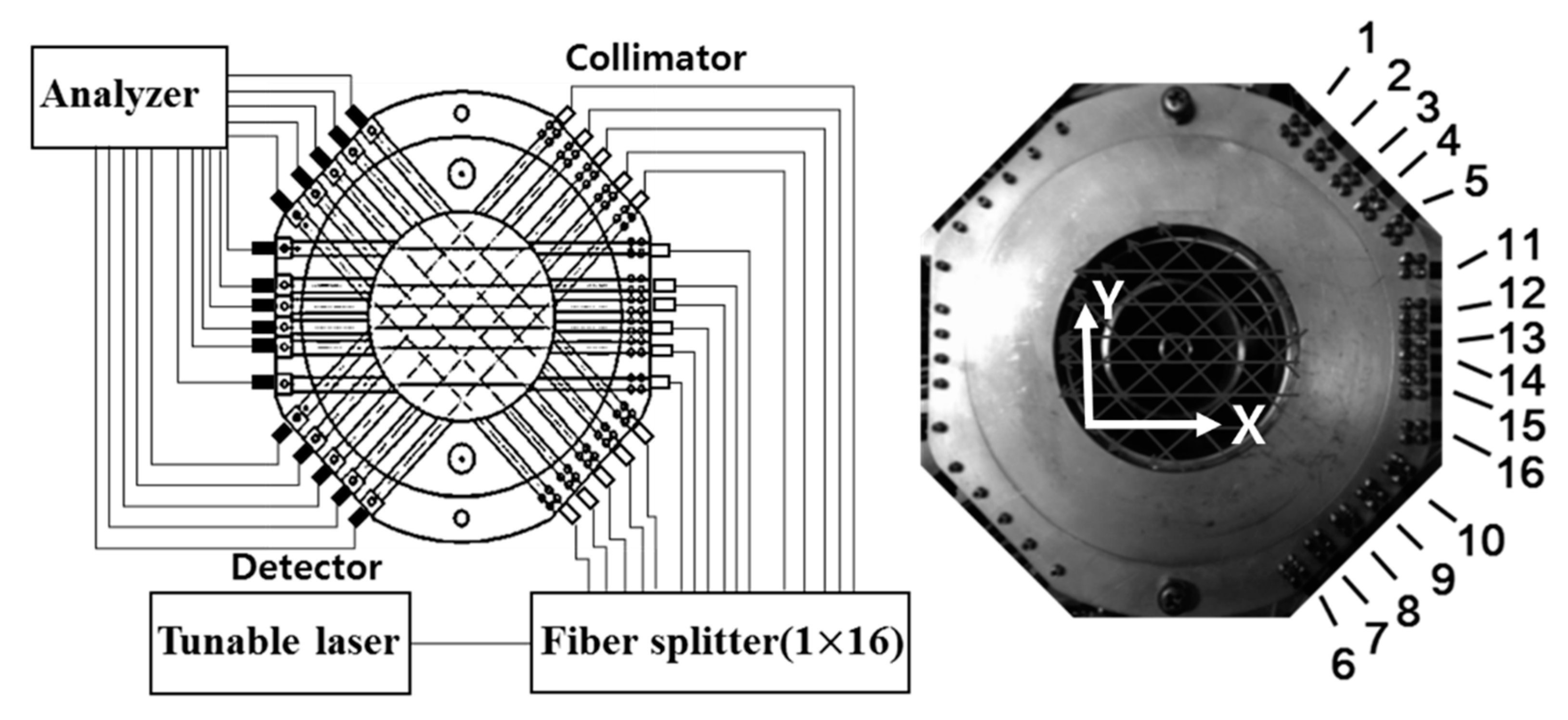
3. TDLAS Tomographic Reconstruction Model (Prototype, Tokushima University, Tokushima, Japan, 2016)

In order to get a two-dimensional temperature distribution via CT calculations, multiple laser beams produced in a form of mesh shown in Figure 3 were constructed by a semiconductor laser, and then all laser intensity information at the grid points of the mesh was reconstructed theoretically using the experimental absorption spectra.

The signal intensity of the absorption lines of the laser pass j is can be expressed by the following Equation (2).

$$A_{\lambda ,j}=-{\displaystyle \sum _i{n}_i\cdot L_{i,j}\cdot {\alpha }_{\lambda ,i}}$$

(2)

Here, A_λ,j is the integrated absorbance of wavelength λ in the path j, α_λ,i is the absorption coefficient of wavelength λ inside a grid i on the path and is dependent upon the temperature and the density of species. L_i,j is the path length inside the grid i.

Figure 4 shows how the temperatures and the concentrations at the grids of the mesh in Figure 3 are obtained in CT calculations.

In the CT process, it is important to adopt the initial values for the temperatures and the concentrations at all grids. In this study, CSLOS (corrective summation of line of sight) method has been adopted. In this method, all absorption signals passing at a grid are added and they are used as the experimental spectra at all grids. The initial values of temperature and concentration at the grids have been installed considering the length and the location of the laser lines. At the initial stages of CT calculation, the initial values obtained by the CSLOS method are used for the calculation of the SMART algorithm, in which Equation (3) is used for the calculation of the absorption coefficients α_λ,i.

$${\alpha }_{\lambda ,i}{}^{k+1}={\alpha }_{\lambda ,i}{}^k\cdot exp\left({\displaystyle \sum _{j=1}^J\frac{L_{ij}}{{\displaystyle \sum _{i=1}^I{L}_{ij}}}\cdot log\frac{A_{\lambda ,j}}{{\displaystyle \sum _{i=1}^I{\alpha }_{\lambda ,i}\cdot L_{ij}}}}\right)$$

(3)

The SMART algorithm is based on a combination product of algebraic reconstruction. This is an iterative calculation approach that allows a cross-entropy minimization. It has been mainly used to reduce convergence time in iterative calculations.

4. Estimation of Initial Temperature and Performance Evaluation

Estimation of proper initial temperature value has a great influence on the result of tomography calculation. Inappropriate initial values lead to the calculation in the diverging direction. It is difficult to determine an initial temperature value from an unknown temperature field. Also, finding the optimum value from an arbitrary temperature value will take a lot of computation time. In this study, initial values were calculated using SLOS (summation of line of sight) and CSLOS (corrective summation of line of sight) method. It is to calculate the initial temperature by calculating the ratio of the integrated absorption amount of the wavelength (#1, #2) about the laser crossing each cell and using the intensity ratio of Figure 2b. It is expressed by the following Equations (4) and (5).

$$SLOS=\frac{A_{\#1,j1}+A_{\#1,j2}}{A_{\#2,j1}+A_{\#2,j2}}$$

(4)

$$CSLOS=\frac{\frac{A_{\#1,j1}}{L_{j1}}+\frac{A_{\#1,j2}}{L_{j2}}}{\frac{A_{\#2,j1}}{L_{j1}}+\frac{A_{\#2,j2}}{L_{j2}}}$$

(5)

Here, j1 and j2 are laser beams passing through each cell. The CSLOS method considers the length of laser path compared with the SLOS method. In the case where there is a lot of information on intersecting lasers, the more accurate initial temperature can be calculated.

Once the initial absorption spectra are obtained by the use of SLOS and CSLOS, the absorption coefficients represented by Equation (3) are calculated iteratively until the differences between the theoretical absorbance and the experimental absorbance using the MSE (mean square error) function as shown in Equation (6) are minimized so that the final temperature and concentration are decided. During iterative calculations, all theoretical spectra were normalized with maximum intensity.

$$Error={\displaystyle \sum {\left\{{(A_{\lambda ,j})}_{theory}-{(A_{\lambda ,j})}_{experiment}\right\}}^2}$$

(6)

5. Experimental Setup

Figure 5 shows the experimental setup. The absorption spectra of H₂O in a flame burner have been measured. The burner has a double-tube structure composed of a sintered bronze filter and external piping. Methane (CH₄) gas has been used as fuel and it has been mixed with air supplied through a sintered bronze filter. The diameter of the main burner tube is 6 mm. The 16 path CT-TDLAS measurement cells as shown in Figure 6 have been set at the position 95 mm above the burner. The experimental parameters are summarized in

Table 1. Experimental parameters.

Combustion Fuel	Methane (L/min)	Dry Air (L/min)	Around Air (L/min)	All Air: Dry Air + Around Air (L/min)
Methane-Air premixed flame	0.74	3.4	96.6	100

.

A DFB (distributed feedback) diode laser (NTT Electronics Co., NLK1E5GAAA) of which working wavelength is 1388 nm with a scanning range of 0.6 nm was used to get H₂O gas absorption spectra. In order to measure simultaneous 2-dimensional absorption spectra a 16-path cell as shown in Figure 6 has been used. Laser paths have 7 mm to 12.3 mm spacing with each other for covering 2-dimensional space. The laser beam has been separated by the use of an optical fiber splitter (OPNETI CO., SMF-28e 1310 nm SWBC 1 × 16). Then, the separated 16 beams pass through 16 collimators (THORLABS Co., 50-1310-APC) to attain focused light intensity. The intensity of the transmitted light has been detected by 16 photodiodes (Hamamatsu Photonics and G8370-01), and they have scanned with 1 kHz and have been recorded onto the recorder (HIOKI E.E. Co., 8861 Memory Highcoda HD Analog16). The detected signals have been amplified using the amplifier (Stanford Research Systems, SR445A).

For temperature comparisons, the temperatures at the same position of the laser 16-path were also measured by one thermocouple with a diameter of 100 μm (ANBE SMT Co., BM-100-100-050).

6. Results and Discussion

In this study, three absorption lines located at 1388.139 nm (#1), 1388.328 nm (#2) and 1388.454 nm (#3) have been chosen for the calculation of temperature and concentration of H₂O. Absorption spectra of H₂O at 1388–1388.6 nm in the 16-path cell have been measured by the CT-TDLAS system shown in Figure 6.

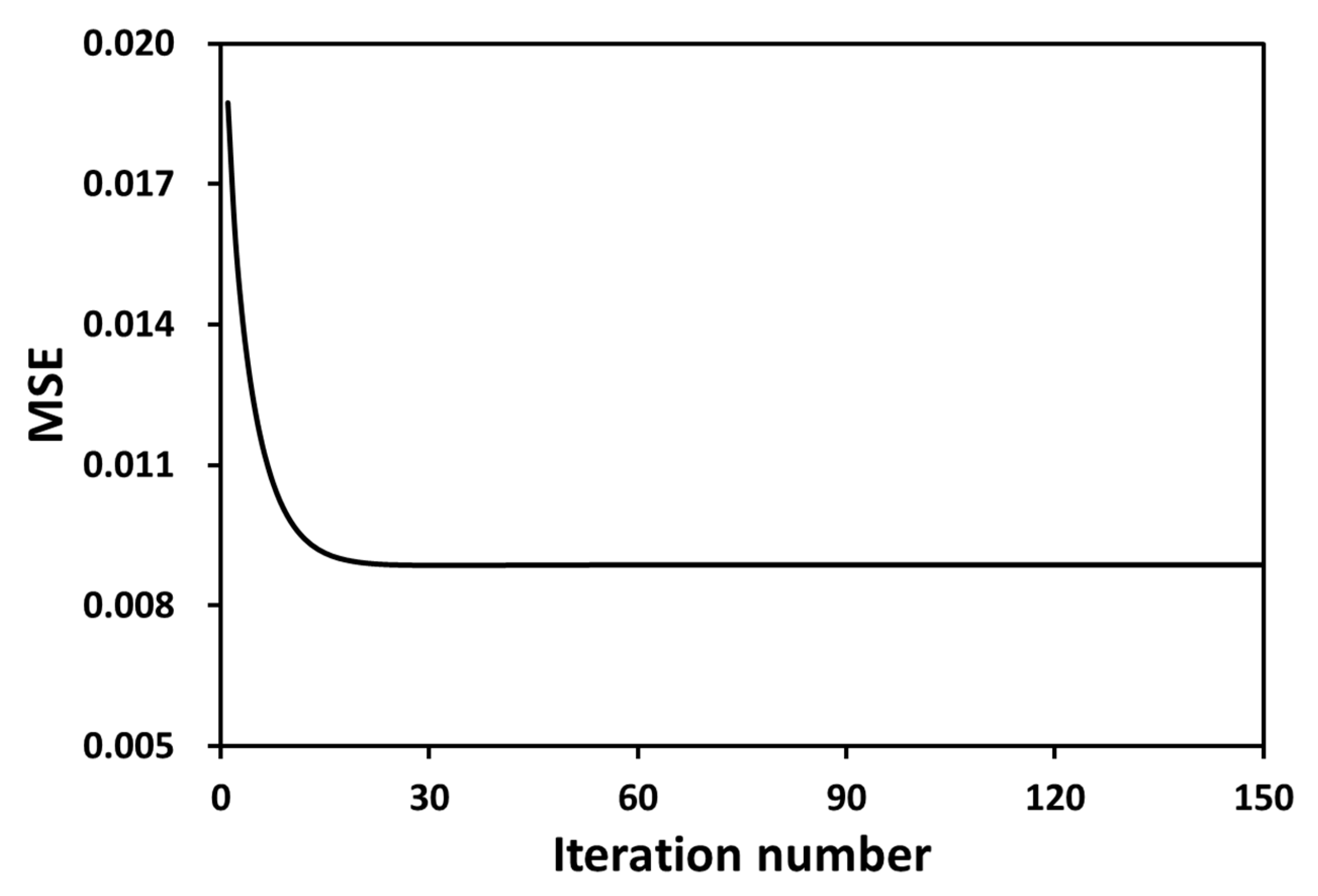
6.1. Optimization for TDLAS

The cause of the error in TDLAS is the disagreement between the theory and experiment. The discrepancies between the original virtual data and the TDLAS calculation data are not so large, and it would be also improved by revising the theoretical spectroscopic data [22]. In addition, it is important to evaluate CT algorithm errors [18,23] together with the evaluation of these spectroscopic errors. The CT algorithm error is according to the shape of the temperature and concentration distributions, and the error tends to increase when the shape is complicated. In actual use of the optical experimental apparatus, the process of reducing the error between the theory and actual experiment is important. It is directly measured by changing the temperature and pressure of the target gas to be measured, and it can be corrected by contrast with the theoretical value. Figure 7 shows the comparisons between the temperatures measured by the TDLAS and by the thermocouple. At the temperature range of 300 K to 800 K, the absorption intensities obtained by a calibration process have been used, in which the concentration of H₂O, the temperature and the pressure could be controlled in a cell [24,25]. At the temperature range higher than 800 K, the absorption intensities obtained by a flat flame burner test [22] performed under the temperature range from 1244 K to 1264 K have been used. Using these results, the HITRAN database over 800 K has been modified for the actual TDLAS calculations. It can be said that the temperature measured by the thermocouple and the temperature calculated by the TDLAS shows a good agreement, revealing high accuracy.

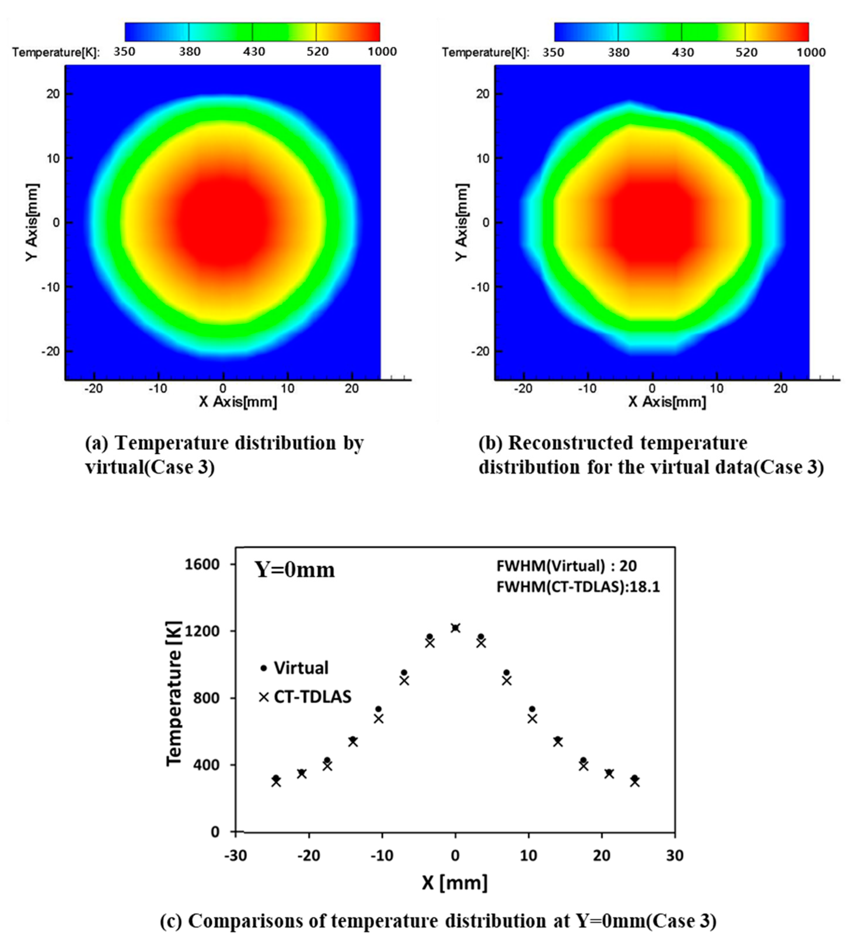
6.2. Estimation of Initial Temperature and the Spatial Resolution Evaluate for CT-TDLAS

The temperature distribution of a virtual flame was generated by the use of Gaussian function at the temperature range of 280 K to 1200 K. The virtual temperature profiles having three different FWHM (full width at half maximum) values (10 mm, 15 mm, 20 mm) have been generated, and the profiles have been reconstructed by CT-TDLAS using those virtual data. In order to evaluate the initial temperature of the CT-TDLAS, MSE has been tested. Figure 8 shows the result of MSE evaluation for the case of

Table 2. The spatial resolution evaluated for the virtual data.

Case No.	FWHM (Virtual) [mm]	FWHM (CT-TDLAS) [mm]	SSD	ZNCC
Case 1	10	16.9	0.14785	0.83801
Case 2	15	17.7	0.05381	0.97191
Case 3	20	18.1	0.01962	0.99907

(Case 3). It can be seen that CSLOS method has better performance than SLOS method for initial value calculation. The minimum error value by the CSLOS method was $3.26\times {10}^{-3}$.

In order to evaluate the spatial resolution of the CT-TDLAS, three factors have been tested. The first one is the FWHM. Then, the FWHM values of the reconstructed temperature profiles by CT-TDLAS have been compared with those of the virtual temperature profiles. The second one is SSD (sum of squared difference). The SSD value has been defined by Equation (11). If the SSD value is close to “0”, the two profiles are almost the same patterns. The third one is ZNCC (zero-mean normalized cross-correlation) value shown in Equation (12). If this value is close to “1”, the virtual data and the data obtained by CT-TDLAS are similar patterns. That is, the correlation between the two values is very high.

$$SSD=\sqrt{\frac{{\displaystyle \sum _{i=0}^{N-1}{\displaystyle \sum _{j=0}^{M-1}{\left\{{(T_{i,j})}_{virtual}-{(T_{i,j})}_{CT–TDLAS}\right\}}^2}}}{NM}}/T_R$$

(11)

$$ZNCC=\frac{{\displaystyle \sum _{i=0}^{N-1}{\displaystyle \sum _{j=0}^{M-1}\left\{{(T_{i,j}-\overline{T})}_{virtual}\times {(T_{i,j}-\overline{T})}_{CT–TDLAS}\right\}}}}{\sqrt{{\displaystyle \sum _{i=0}^{N-1}{\displaystyle \sum _{j=0}^{M-1}{(T_{i,j}-\overline{T})}_{virtual}{}^2\times {\displaystyle \sum _{i=0}^{N-1}{\displaystyle \sum _{j=0}^{M-1}{(T_{i,j}-\overline{T})}_{CT–TDLAS}{}^2}}}}}},\begin{array}{cc}& \end{array}\overline{T}=\frac{{\displaystyle \sum _{i=0}^{N-1}{\displaystyle \sum _{j=0}^{M-1}{T}_{i,j}}}}{NM}$$

(12)

Here, $T_{i,j}$ is the temperature at each point in a calculation area, $T_R$ is the representing temperature (the max temperature of virtual data), N is the total number of meshes along X-axis in the calculation area, and M is the total number of meshes along Y-axis in the calculation.

Table 2 shows the comparison of the above three values between the virtual data and the data obtained by CT-TDLAS for three different cases, of which FWHM is 10 mm, 15 mm, and 20 mm. It can be said that the SSD values for the three cases are less than 5% (13.155 K/280 K) at most. This implies that the discrepancy between the original virtual data and the data obtained by CT-TDLAS calculation is very small, showing that the present calculation approach is appropriate. Figure 9a,b shows the results of the case 3. Figure 9c shows the temperature profiles at the centerline of the calculation area for the virtual one and the CT-TDLAS calculation results.

The spatial resolution of CT is related to the spatial density of the calculation grid. The number of the grid in a CT calculation area and the distance between each grid is known as the sampling interval, which is a function of the accuracy of the CT calculation. In this study used a spatial resolution of the CT is about 18.1 mm (Case3) shown in Table 2. This result is due to the configuration of the CT calculation grid considering a position of laser path in the whole measurement area. The composition of CT grid used 10 × 10 for the measurement area with a diameter of 70 mm. The larger the FWHM value of the virtual temperature field is higher the estimation ability with respect to temperature, and the smaller the FWHM value is the lower the estimation ability of the temperature. It can be confirmed by SSD (sum of squared difference), ZNCC (zero-mean normalized cross-correlation) method.

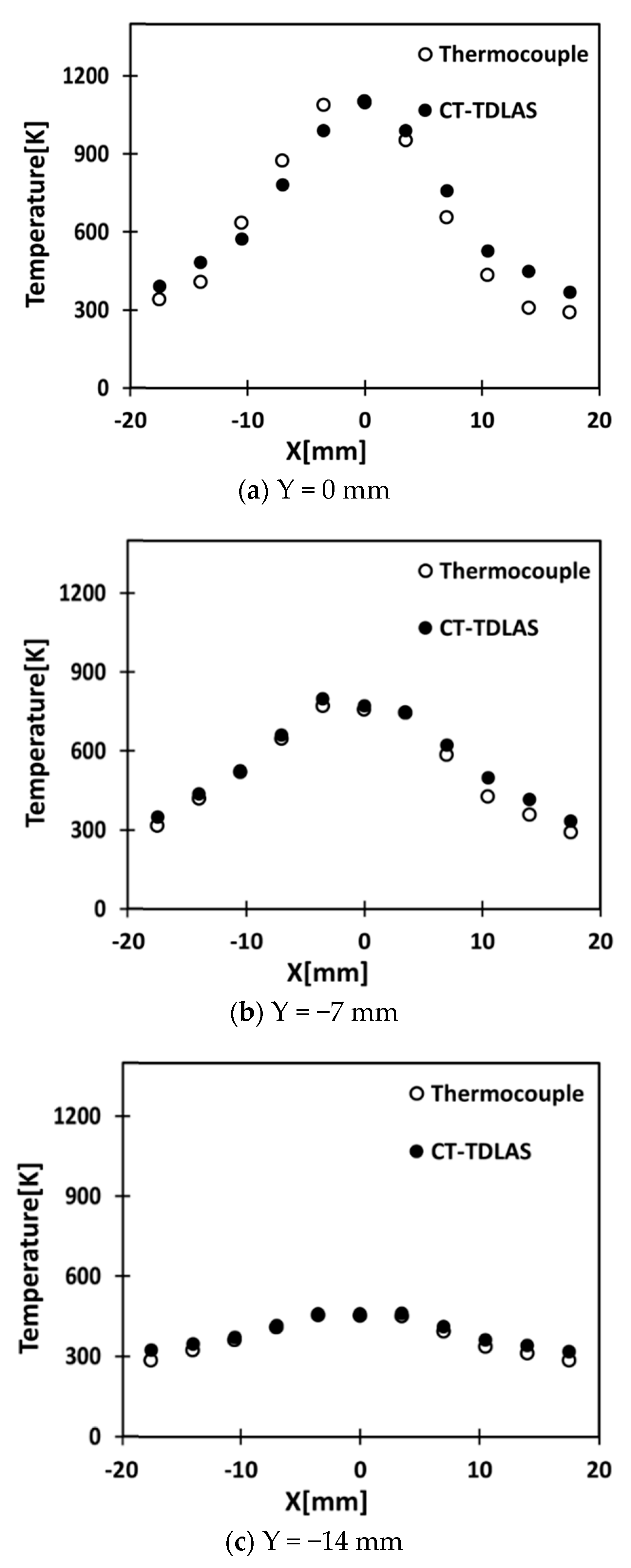
6.3. Experimental Tests

Figure 10 shows the 2-dimensional temperature field measured by one thermocouple experiment. This shows the reconstructed temperature calculated at the grids of 2 mm intervals of the measurement cell. It can be seen that the temperature at the center area is relatively high temperature.

Figure 11 shows the minimum MSE of the absorption intensities on all grids when the CSLOS initial values have been adopted. The minimum value was $8.86\times {10}^{-3}$.

Figure 12a,b shows the results obtained by the CT-TDLAS, in which the SMART algorithm has been adopted. It can be seen that the temperature distribution is similar to the distribution measured by the thermocouple as shown in Figure 10, revealing that the temperature calculated by the current approach of CT-TDLAS is validated. However, there is some irregular distribution in the concentration field. This is due to the influences of the boundary grids.

Figure 13a–c shows the comparisons of the results measured by the thermocouple and calculated by the CT-TDLAS for three different Y locations at Y = 0 mm, Y = −7 mm, and Y = −14 mm. It can be seen that the discrepancies between the temperature measured by the thermocouple and the temperature calculated by the CT-TDLAS are quite small at outside locations from the flame burner center.

Table 3. The spatial resolution evaluated for the real flame data.

Measurement Type	SSD	ZNCC
CT-TDLAS	0.05737	0.9480

shows the spatial resolution between thermocouple results and CT-TDLAS results at a temperature. It can confirm the reliability of CT-TDLAS results from these quantitative values.

7. Conclusions

The measurements for temperature distribution have been performed by a thermocouple. The temperature distribution has been reconstructed by the SMART algorithm and the results have been compared with those by the thermocouple giving the following summary.

• It can be seen that the CSLOS method has better performance than the SLOS method for initial value calculation. Therefore, a CSLOS method has been adopted to get initial values. It has been experimentally shown that this approach is appropriate for choosing the initial values for performing iterative calculations with the experimental absorption spectra of the CT-TDLAS.
• In order to evaluate the performance of the adopted CT-TDLAS algorithm, three parameters, FWHM, SSD, and ZNCC, have been adopted, by which the adopted CT-TDLAS algorithm is capable of reconstructing the temperature distribution and the concentration distribution with relatively high accuracy.
• To enhance of the performance of the temperature measurement using the CT-TDLAS, the SMART algorithm has been adopted, and the relative error was 10.12%. This implies that a SMART algorithm is a reliable approach for reconstructing the multiple signals of the CT-TDLAS.
• The discrepancies between the temperature measured by the thermocouple and the temperature calculated by the CT-TDLAS were quite small at outside locations from the flame burner center. However, these discrepancies were relatively larger at the center region (high-temperature area) of the burner. It seems that the major part of the temperature discrepancies was due to the influence of the radiation flux.

References

1. Wang, W.; Lim, C.B.; Lee, K.K.; Yang, S.S. Wireless Surface Acoustic Wave Chemical Sensor for Simultaneous Measurement of CO2 and Humidity. J. Micro/Nanolith. MEMS MOEMS 2009, 8, 031306. [Google Scholar] [CrossRef]
2. Sternhagen, J.D.; Wold, C.E.; Kempf, W.A. A Novel Integrated Acoustic Gas and Temperature Sensor. IEEE Sens. J. 2002, 2, 301–306. [Google Scholar] [CrossRef]
3. Dossi, N.; Toniolo, R.; Pizzariello, A.; Carrilho, E.; Piccin, E.; Battiston, S.; Bontempelli, G. An Electrochemical Gas Sensor based on Paper Supported Room Temperature Ionic Liquids. Lab Chip 2012, 12, 153–158. [Google Scholar] [CrossRef] [PubMed]
4. Fine, G.F.; Cavanagh, I.M.; Afonja, A.; Binions, R. Metal Oxide Semi-Conductor Gas Sensors in Environmental Monitoring. Sensors 2010, 10, 5469–5502. [Google Scholar] [CrossRef] [PubMed]
5. Deguchi, Y. Industrial applications of Laser Diagnostics; Taylor & Francis CRS Press: Boca Raton, FL, USA, 2011; ISBN 9781439853375. [Google Scholar]
6. Zaatar, Y.; Bechara, J.; Khoury, A.; Zaouk, D.; Charles, J.-P. Diode laser sensor for process control and environmental monitoring. Appl. Energy 2000, 65, 107–113. [Google Scholar] [CrossRef]
7. Yamakage, M.; Muta, K.; Deguchi, Y.; Fukada, S.; Iwase, T.; Yoshida, T. Development of Direct and Fast Response Exhaust Gas. Meas. SAE Paper 2008, 20081298. [Google Scholar] [CrossRef]
8. Morthier, G.; Vankwikelberge, P. Handbook of Distributed Feedback Laser Diodes; Artech House Applied Photonics: Boston, FL, USA, 2013; ISBN 978-1608077014. [Google Scholar]
9. Yariv, A.; Yeh, P. Photonics: Optical Electronics in Modern Communications; Oxford University Press: Oxford, UK, 2006; ISBN 9780195179460. [Google Scholar]
10. Kranendonk, L.A.; Walewski, J.W.; Kim, T.; Sanders, S.T. Wavelength-agile sensor applied for HCCI engine measurement. Proc. Combust. Inst. 2005, 30, 1619–1627. [Google Scholar] [CrossRef]
11. Rieker, G.B.; Li, H.; Liu, X.; Liu, J.T.C.; Jeffries, J.B.; Hanson, R.K.; Allen, M.G.; Wehe, S.D.; Mulhall, P.A.; Kindle, H.S.; et al. Rapid measurements of temperature and H2O concentration in IC engines with a spark plug-mounted diode laser sensor. Proc. Combust. Inst. 2007, 31, 3041–3049. [Google Scholar] [CrossRef]
12. Liu, X.; Jeffries, J.B.; Hanson, R.K.; Hinckley, K.M.; Woodmansee, M.A. Development of a tunable diode laser sensor for measurements of gas turbine exhaust temperature. Appl. Phys. B 2006, 82, 469–478. [Google Scholar] [CrossRef]
13. Sumizawa, H.; Yamada, H.; Tonokura, K. Real-time monitoring of nitric oxide in diesel exhaust gas by mid-infrared cavity ring-down spectroscopy. Appl. Phys. B 2010, 100, 925–931. [Google Scholar] [CrossRef]
14. Anderson, T.N.; Lucht, R.P.; Priyadarsan, S.; Annamalai, K.; Caton, J.A. In situ measurements of nitric oxide in coal-combustion exhaust using a sensor based on a widely tunable external-cavity GaN diode laser. Appl. Opt. 2007, 46, 3946–3957. [Google Scholar] [CrossRef] [PubMed]
15. Magnuson, J.K.; Anderson, T.N.; Lucht, R.P. Application of a diode-laser-based ultraviolet absorption sensor for in situ measurements of atomic mercury in coal-combustion exhaust. Energy Fuels 2008, 22, 3029–3036. [Google Scholar] [CrossRef]
16. Kasyutich, V.L.; Holdsworth, R.J.; Martin, P.A. In situ vehicle engine exhaust measurements of nitric oxide with a thermoelectrically cooled. J. Phys. Conf. Seeries 2009, 157, 012006. [Google Scholar] [CrossRef]
17. Wang, F.; Cen, K.F.; Li, N.; Jeffries, J.B.; Huang, Q.X.; Yan, J.H.; Chi, Y. Two-dimensional tomography for gas concentration and temperature distributions based on tunable diode laser absorption spectroscopy. Meas. Sci. Technol. 2010, 21. [Google Scholar] [CrossRef]
18. Ma, L.; Cai, W. Numerical investigation of hyperspectral tomography for simultaneous temperature and concentration imaging. Appl. Opt. 2008, 47, 3751–3759. [Google Scholar] [CrossRef]
19. Wright, P.; Terzija, N.; Davidson, L.; Castillo, S.G.; Garcia-Stewart, C.; Pegrum, S.; Colbourne, S.; Turner, P.; Crossley, S.D.; Litt, T.; et al. High-speed chemical species tomography in a multi-cylinder automotive engine. Chem. Eng. J. 2010, 158, 2–10. [Google Scholar] [CrossRef]
20. Jeon, M.G.; Deguchi, Y.; Kamimoto, T.; Doh, D.H.; Cho, G.R. Performances of new reconstruction algorithms for CT-TDLAS computer tomography-tunable diode laser absorption spectroscopy. Appl. Therm. Eng. 2017, 115, 1148–1160. [Google Scholar] [CrossRef]
21. Rothman, L.S.; Gordon, I.E.; Babikov, Y.; Barbe, A.; Benner, D.C.; Bernath, P.F.; Birk, M.; Bizzocchi, L.; Boudon, V.; Brown, L.R.; et al. The HITRAN2008 Molecular Spectroscopic Database. J. Quant. Spectrosc. Radiat. Transf. 2009, 110, 533–572. [Google Scholar] [CrossRef]
22. Kamimoto, T.; Deguchi, Y.; Kiyota, Y. High temperature field application of two dimensional temperature measurement technology using CT tunable diode laser absorption spectroscopy. Flow Meas. Instrum. 2015, 46, 51–57. [Google Scholar] [CrossRef]
23. An, X.; Kraetschmer, T.; Takami, K.; Sanders, S.T.; Ma, L.; Cai, W.; Li, X.; Roy, S.; Gord, J.R. Validation of temperature imaging by H2O absorption spectroscopy using hyperspectral tomography in controlled experiments. Appl. Opt. 2011, 50, 29–37. [Google Scholar] [CrossRef]
24. Choi, D.W.; Jeon, M.G.; Cho, G.R.; Kamimoto, T.; Deguchi, Y.; Doh, D.H. Performance Improvements in Temperature Reconstructions of 2-D Tunable Diode Laser Absorption Spectroscopy TDLAS. J. Therm. Sci. 2016, 25, 84–89. [Google Scholar] [CrossRef]
25. Kamimoto, T.; Deguchi, Y. 2D Temperature Detection Characteristics of Engine Exhaust Gases Using CT Tunable Diode Laser Absorption Spectroscopy. Int. J. Mech. Syst. Eng. 2015, 1, 109. [Google Scholar] [CrossRef] [PubMed]
Figure 1. Relative intensity of theoretical H2O absorption spectra (1388 nm~1388.5 nm).
Applsci 09 04955 g001
Figure 2. Theoretical temperature dependence H2O absorption spectra.
Applsci 09 04955 g002
Figure 3. Calculation grids for tomographic reconstructions.
Applsci 09 04955 g003
Figure 4. Calculation process of temperature and concentration at all grids in CT-TDLAS.
Applsci 09 04955 g004
Figure 5. Experimental apparatus for 2D temperature measurement in flame burner using CT-TDLAS.
Applsci 09 04955 g005
Figure 6. 16-paths CT-TDLAS measurement cell.
Applsci 09 04955 g006
Figure 7. Comparisons between the temperatures measured by TDLAS and thermocouple.
Applsci 09 04955 g007
Figure 8. MSE (mean square error) comparison for initial temperature (Case 3).
Applsci 09 04955 g008
Figure 9. The spatial resolution test of temperature distribution (Case 3).
Applsci 09 04955 g009
Figure 10. Temperature distribution measured by thermocouple.
Applsci 09 04955 g010
Figure 11. Total MSE variations for the iteration number in case of adopting SMART algorithm.
Applsci 09 04955 g011
Figure 12. Temperature and concentration distributions reconstructed by SMART algorithm.
Applsci 09 04955 g012
Figure 13. Comparisons of temperature distribution at Y = 0mm, −7 mm and −14 mm calculated by the SMART algorithm of CT-TDLAS and measured by the thermocouple.
Applsci 09 04955 g013