A Time Integration Method Based on Galerkin Weak Form for Nonlinear Structural Dynamics

Abstract

This paper presents a step-by-step time integration method for transient solutions of nonlinear structural dynamic problems. Taking the second-order nonlinear dynamic equations as the model problem, this self-starting one-step algorithm is constructed using the Galerkin finite element method (FEM) and Newton–Raphson iteration, in which it is recommended to adopt time elements of degree m = 1,2,3. Based on the mathematical and numerical analysis, it is found that the method can gain a convergence order of 2m for both displacement and velocity results when an ordinary Gauss integral is implemented. Meanwhile, with reduced Gauss integration, the method achieves unconditional stability. Furthermore, a feasible integration scheme with controllable numerical damping has been established by modifying the test function and introducing a special integral rule. Representative numerical examples show that the proposed method performs well in stability with controllable numerical dissipation, and its computational efficiency is superior as well.

1. Introduction

The step-by-step time integration method is the most commonly used numerical method for transient analysis of nonlinear dynamics, and can in general be classified into an explicit and implicit scheme. For the explicit integration algorithm, it is not required to solve coupled equations in each time step, and this method is more suitable for determining solutions of wave propagation problems. While for the implicit algorithm, although the requirement for solutions of coupled equations in each time step makes it expensive, it still has been widely used in solid mechanics and structural engineering because of the superior numerical stability. In fact, it may often occur that an implicit algorithm of unconditional stability in linear problems fails to give a stable response for some nonlinear problems. For example, significant instability may appear in the trapezoidal rule [1] when it is used for the evaluation of large deformation problems and long time range responses [2,3,4,5].

For linear dynamics, the stability of an integration algorithm can be estimated by spectral analysis, whereas in nonlinear dynamics spectral analysis is only one of the requirements to remain stable, and the conservation or decay of total energy within a time step interval should be the very sufficient condition for effective solutions [3]. From this point of view, the time integration method can be classified into three categories: One of numerical dissipation, one of enforced conservation of energy and one of algorithmic conservation of energy. Firstly, the algorithm belonging to the numerical dissipation category uses numerical dissipation to achieve energy conservation or decay. For example, numerical damping of high-order-frequency can be introduced into the Newmark method with $\gamma >1/2$, however, in this case, the method only possesses an accuracy of the first order. For another example, in the HHT-$\alpha$ [6] method and generalized-$\alpha$ [7] method, the numerical accuracy has been improved to the second order and controllable numerical damping has been introduced as well. For such methods, the suitable selection of parameters turns out to be the key to achieving effective energy decay. Secondly, the algorithm of enforced conservation of energy was first proposed by Huges et al. [8]. It is formed by introducing Lagrange multipliers into the trapezoidal integral method, and then achieves the target to satisfy energy conservation. However, the Newton–Raphson iteration may sometimes fail in the end [9]. The third kind of algorithm with algorithmic conservation of energy [10] was first proposed by Simo and Tarnow [11]. Its basic idea comes from the adjustment of the mid-point rule, which can realize energy conservation by expressing the stress tensor of the midpoint of the time interval in terms of the average of the stress tensors at the initial time and the end time of that time interval [12,13,14,15].

Besides of the finite difference method, this is one of the main numerical methods for initial value problems (IVPs). In recent years, many alternative finite element methods (FEMs) for IVPs have been developed [16], which are as well-known as time FEM. According to the different ways of construction, the time FEM can be roughly classified into three kinds: (1) Constructed by Gurtin variational principle, which transforms the initial-boundary value problem into the equivalent boundary value problem (BVP) by means of Laplace positive and inverse transformation [17,18]; (2) Constructed by Hamilton’s variational principle or Hamilton’s law of variation [19,20,21], in which Bailey [22,23], Simikins [24], and Borri [25] have made important achievements successively and; (3) Constructed by the weighted residual method, and is what we use in the present paper.

For time FEMs established by the weighted residual method, the trial functions commonly used involve Lagrange interpolation polynomials [26], linear/quadratic polynomials [27,28], Taylor expansion [29,30], or Taylor formulae [31,32]. Zienkiewicz has developed a framework for constructing a direct integration method based on weighted residuals of the governing equations [33]. Xianghua Xing [34] has proposed a direct integration method based on Galerkin weak form for linear dynamics, named the GW method. Hoff and Pahl have formed a one-step time FEM by setting acceleration, velocity, and displacement to be linear, quadratic, and cubic Taylor polynomials, respectively, which has been applied to both linear [29] and nonlinear [35] structural dynamic problems. Betsch P has proposed a time FEM with inherent energy conservation based on Hamilton’s canonical equations combined with the continuous Galerkin (cG) method [36], which has been successfully applied to nonlinear elastodynamics [37].

Different from the traditional Galerkin FEMs with continuous state variables in the time domain, Reed and Hill [38] and Lasaint and Raviart [39], have proposed the discontinuous Galerkin (dG) FEM for time-dependent problems by using discontinuous trial and test functions. The transition variables between two elements are discontinuous, based on which a step-by-step integration method with energy decay [40] was established.

Up to now, the development of a reliable and effective numerical algorithm for nonlinear dynamic equations is still a core research subject in structural dynamics [5,10]. In the present paper, a time integration method based on Galerkin method for solving linear/nonlinear IVPs is proposed and presented. A set of implicit time integration schemes have been derived with time elements of degree m = 1,2,3 being used. By means of the Newton–Raphson method, the computational iterative procedure is formed, and then the accuracy and numerical stability of the algorithm are studied and analyzed, after which an integration scheme with controllable numerical damping is constructed for linear elements. Typical numerical examples, including the simple pendulum, a long span planar skeletal structure, and a cantilever beam, are solved to test the characteristics of the proposed method against some other representative time integration schemes including the trapezoidal rule, Newmark method ($\gamma = 1/2, \beta = 1/6$) [1], Wilson $\theta$-method ($\theta = 1.4$) [41], and Bathe method ($\gamma = 1/2$) [5]. The results demonstrate the merits of the proposed method in terms of both stability and efficiency. In the following sections of the paper, these contents will be presented one by one.

2. Basic Principle

2.1. Governing Equations and Iterative Schemes

For nonlinear dynamic problems in solid mechanics and structural engineering, discretization in the space dimension generally results in the following governing equations in the time domain, which are named dynamic equations hereinafter:

$$\{\begin{array}{l}M\ddot{u}+f_d(\dot{u})+f_s(u)=f_{ext},0<t\le t_f\\ u(0)=u_0,\dot{u}(0)={\dot{u}}_0\end{array}$$

(1)

where $u\equiv u(t)$ is the unknown vector of vibration displacements/rotations, $M$ is the mass matrix, $f_d$ is the vector of damping forces depending on velocity $\dot{u}\equiv \mathrm{d}u(t)/\mathrm{d}t$, $f_s$ is the vector of resilience depending on displacement, and $f_{ext}$ represents the vector of externally applied forces. The solution domain is supposed to be $(0,t_f]$, with $u_0$ and ${\dot{u}}_0$ being the given initial condition vectors.

When $f_d$ or $f_s$ is the nonlinear function of $\dot{u}$ or $u$, Equation (1) is a typical IVP of nonlinear ordinary differential equations (ODEs). A common strategy for solving such ODEs is to transform them into linear equations and then perform iteration. Thus the Newton–Raphson method is first applied to Equation (1) which results in the following linearized ODEs:

$$\{\begin{array}{l}M{\ddot{u}}^{(k+1)}+{\overline{C}}^{(k)}{\dot{u}}^{(k+1)}+{\overline{K}}^{(k)}{u}^{(k+1)}=f_{\mathrm{ext}}-f_{\mathrm{int}}^{}{}^{(k)},t_n\le t\le t_{n+1}\\ u^{(k+1)}(t_n)=u_n,{\dot{u}}^{(k+1)}(t_n)={\dot{u}}_n\end{array}$$

(2)

where

$${\overline{C}}^{(k)}={(\frac{\partial f_d}{\partial \dot{u}})|}_{{\dot{u}}^{(k)}},\text{}{\overline{K}}^{(k)}={(\frac{\partial f_s}{\partial u})|}_{u^{(k)}}$$

(3)

$$f_{\mathrm{int}}^{}{}^{(k)}={(f_d{}^{(k)}|}_{{\dot{u}}^{(k)}}-{\overline{C}}^{(k)}{\dot{u}}^{(k)})+{(f_s{}^{(k)}|}_{u^{(k)}}-{\overline{K}}^{(k)}{u}^{(k)}).$$

(4)

Here $u^{(k)}$, ${\dot{u}}^{(k)}$, and ${\ddot{u}}^{(k)}$ are quantities obtained in the k-th iteration step (k = 0,1,2,…), the tangential damping matrix ${\overline{C}}^{(k)}$, tangential stiffness matrix ${\overline{K}}^{(k)}$ and internal force vector $f_{\mathrm{int}}^{(k)}$ are functions of time. For convenience, we omit the superscript ‘k’ in Equation (2) temporarily and denote $f=f_{\mathrm{ext}}-f_{\mathrm{int}}^{}$. Then, Equation (2) can be written into the following simplified form, which is the main solution target of the next subsection:

$$\{\begin{array}{l}M\ddot{u}+\overline{C}\dot{u}+\overline{K}u=f,t_n\le t\le t_{n+1}\\ u(t_n)=u_n,\dot{u}(t_n)={\dot{u}}_n\end{array}.$$

(5)

2.2. Galerkin Finite Element Method

To solve the linear IVP of ODEs in Equation (5), a time-domain FEM based on the Galerkin weak form [25,34,42] was used in the present paper. Let $v\in H_v^1$ and $u^h\in H_E^1$ denote the test function and the trial function, respectively. The weighted residual weak form of Equation (5) might be established in time interval $[t_n,t_{n+1}]$ as follows:

$${\displaystyle {\int }_{t_n}^{t_{n+1}}{v}^T(M{\ddot{u}}^h+\overline{C}{\dot{u}}^h+\overline{K}{u}^h)\mathrm{d}t}={\displaystyle {\int }_{t_n}^{t_{n+1}}{v}^{T}f\mathrm{d}t}$$

(6)

where $H_E^1$ and $H_v^1$ represent the trial function space and the test function space, respectively.

Taking $[t_n,t_{n+1}]$ as a typical time element of the FEM with $\Delta t=t_{n+1}-t_n$, as shown in Figure 1, the m-degree polynomials are adopted as the trial function and test function defined on this typical element, i.e.,:

$$u^h=Nd={\displaystyle \sum _{i=1}^{m+1}{N}_i(t)d_i}$$

(7a)

$$v^h=N{d}_v={\displaystyle \sum _{i=1}^{m+1}{N}_i(t)v_i}$$

(7b)

where the shape functions $N_i(t)$ (i = 1, 2, …, m + 1) are Lagrange polynomials, the shape function matrix $N=[N_{1}I,N_{2}I,\cdots ,N_{m+1}I]$, and I is the unit matrix, $d={\{d_1^T{d}_2^T\cdots d_{m+1}^T\}}^T$, and $d_i$ with $d_1=u_n$, $d_{m+1}=u_{n+1}$ is the nodal displacement vector at time ${\overline{t}}_i$, and $d_v={\{v_1^T{v}_2^T\cdots v_{m+1}^T\}}^T$ is the vector of nodal test displacements.

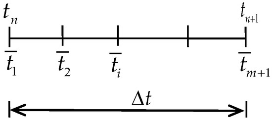
Figure 1. A time element of degree m.

Substituting Equation (7b) into Equation (6), because of the arbitrariness of test displacement vector $d_v$, the following equation can be derived:

$${\displaystyle \underset{t_n}{\overset{t_{n+1}}{\int }}{N}^{T}M{\ddot{u}}^h\mathrm{d}t}+{\displaystyle \underset{t_n}{\overset{t_{n+1}}{\int }}{N}^T\overline{C}{\dot{u}}^h\mathrm{d}t}+{\displaystyle \underset{t_n}{\overset{t_{n+1}}{\int }}{N}^T\overline{K}{u}^h\mathrm{d}t}={\displaystyle \underset{t_n}{\overset{t_{n+1}}{\int }}{N}^{T}f\mathrm{d}t}.$$

(8)

After implementing integration by parts for the first term of Equation (8), which is:

$${\displaystyle \underset{t_n}{\overset{t_{n+1}}{\int }}{N}^{T}M{\ddot{u}}^h\mathrm{d}t}=({N^{T}M{\dot{u}}^h)|}_{t_n}^{t_{n+1}}-{\displaystyle \underset{t_n}{\overset{t_{n+1}}{\int }}{\dot{N}}^{T}M{\dot{u}}^h\mathrm{d}t}=N{(t_{n+1})}^{T}M{\dot{u}}_{n+1}-N{(t_n)}^{T}M{\dot{u}}_n-{\displaystyle \underset{t_n}{\overset{t_{n+1}}{\int }}{\dot{N}}^{T}M{\dot{u}}^h\mathrm{d}t}$$

(9)

where ${\dot{u}}_{n+1}$ and ${\dot{u}}_n$ represent the velocity at $t_{n+1}$ and $t_n$, respectively. Substituting Equation (7a) into Equation (8), and then taking a time coordinate mapping from $t\in [t_n,t_{n+1}]$ to $\zeta \in [-1,1]$, the following algebraic equations are yielded:

$$(\frac{-4}{\Delta t^2}{}^{m}K+\frac{2}{\Delta t}{}^{c}K+{}^{k}K)d^{}+\frac{2M}{\Delta t}(N{(1)}^T{\dot{u}}_{n+1}-N{(-1)}^T{\dot{u}}_n)=P$$

(10)

with

$${}^{m}K={\displaystyle {\int }_{-1}^1{\dot{N}}^{T}M\dot{N}}\mathrm{d}t,{}^{c}K={\displaystyle {\int }_{-1}^1{N}^T\overline{C}(\zeta )\dot{N}}\mathrm{d}t$$

(11)

$${}^{k}K={\displaystyle {\int }_{-1}^1{N}^T\overline{K}(\zeta )N}\mathrm{d}t,P={\displaystyle {\int }_{-1}^1{N}^{T}f\mathrm{d}t}$$

(12)

denoting

$$K=\frac{-4}{\Delta t^2}{}^{m}K+\frac{2}{\Delta t}{}^{c}K+{}^{k}K.$$

(13)

Equation (10) is equivalent to the equation:

$$Kd+\frac{2M}{\Delta t}(N{(1)}^T{\dot{u}}_{n+1}-N{(-1)}^T{\dot{u}}_n)=P$$

(14)

which could further be written into the following tensor notation form:

$$K_{ij}^{}{d}_j^{}+{\delta }_{im+1}\frac{2M}{\Delta t}{\dot{u}}_{n+1}^{}=P_i^{}+{\delta }_{i1}\frac{2M}{\Delta t}{\dot{u}}_n^{}(i,j= 1,2, \dots ,m+ 1)$$

(15)

with ${\delta }_{im+1}$ and ${\delta }_{i1}$ being the Kronecker delta function and:

$$K_{ij}^{}={\displaystyle \underset{-1}{\overset{1}{\int }}\left(-\frac{4}{\Delta t^2}{\dot{N}}_i^{}M{\dot{N}}_j+\frac{2}{\Delta t}{N}_i^{}\overline{C}{\dot{N}}_j+N_i^{}\overline{K}{N}_j\right)\mathrm{d}\zeta }$$

(16)

$$P_i^{}={\displaystyle \underset{-1}{\overset{1}{\int }}{N}_{i}f}\mathrm{d}\zeta .$$

(17)

As a result, Equation (15) is the step-by-step solution formula derived from the Galerkin FEM to solve the time-dependent problem in Equation (5).

2.3. Numerical Integration

In Equation (14), there exists a number of integral terms. Since the integral accuracy of these terms might affect the numerical stability of the whole algorithm, the scheme of Gauss numerical integration is briefly described and discussed in this subsection.

With ${\omega }_l$ and ${\zeta }_l$ denoting the Gaussian integral coefficients and locations of $n_l$ Gaussian points in $[-1,1]$, Equations (16) and (17) might be expressed as:

$$\begin{array}{c}{K}_{ij}^{}=-\frac{4}{\Delta t^2}{\displaystyle \sum _{l=1}^{n_l}{\overline{\omega }}_l{\dot{N}}_i^{}({\overline{\zeta }}_l)M{\dot{N}}_j({\overline{\zeta }}_l)}+\frac{2}{\Delta t}{\displaystyle \sum _{l=1}^{n_l}{\overline{\omega }}_l{N}_i^{}({\overline{\zeta }}_l)\overline{C}({\dot{u}}_l){\dot{N}}_j({\overline{\zeta }}_l)}\\ +{\displaystyle \sum _{l=1}^{n_l}{\overline{\omega }}_l{N}_i^{}({\overline{\zeta }}_l)\overline{K}(u_l)N_j({\overline{\zeta }}_l)}\end{array}$$

(18)

$$P_i^{}={\displaystyle \sum _{l=1}^{n_l}{\overline{\omega }}_l{N}_i^{}({\overline{\zeta }}_l)f({\dot{u}}_l,u_l)}$$

(19)

where

$$u_l=N({\overline{\zeta }}_l)d={\displaystyle \sum _{i=1}^{m+1}{N}_i({\overline{\zeta }}_l)d_i}$$

(20)

$${\dot{u}}_l=\dot{N}({\overline{\zeta }}_l)d={\displaystyle \sum _{i=1}^{m+1}{\dot{N}}_i({\overline{\zeta }}_l)d_i}.$$

(21)

2.4. Iterative Algorithm

Equation (15) is a general step-by-step solution formula for the linear IVP of Equation (5) with time finite elements of degree m, where m can be any positive integer, in theory. However, in practice, examples have shown that the formulae with m = 1,2,3, i.e., linear, quadratic, and cubic time elements, are more pragmatic and sufficiently effective, with no need that m to be much higher. Therefore, the detailed computation schemes of Equation (15) for m = 1,2,3 are given in this subsection, and then the entire iterative algorithm of the Galerkin time FEM is established for the solution of the nonlinear IVP in Equation (1).

For the linear Lagrange time element, there are only two nodes in the single element in Figure 1, i.e., ${\overline{t}}_1=t_n$ and ${\overline{t}}_2=t_{n+1}$. In this case, Equation (14), the step-by-step solution formula of the linear IVP, can be expressed as:

$$\left[\begin{array}{l}{K}_{11}^{}{K}_{12}^{}\\ K_{21}^{}{K}_{22}^{}\end{array}\right]\left\{\begin{array}{l}{u}_n^{}\\ u_{n+1}^{}\end{array}\right\}+\frac{2M}{\Delta t}(\left\{\begin{array}{l}0\\ {\dot{u}}_{n+1}\end{array}\right\}-\left\{\begin{array}{l}{\dot{u}}_n\\ 0\end{array}\right\})=\left\{\begin{array}{l}{P}_1^{}\\ P_2^{}\end{array}\right\}$$

(22)

where $u_n^{}$ and ${\dot{u}}_n^{}$ are the initial displacement and velocity at time $t_n$, respectively. Furthermore, the final solution formula with the omitted iteration symbol “k” being added can be expressed as:

$$\left[\begin{array}{l}{K}_{12}^{(k)}0\\ K_{22}^{(k)}\frac{2M}{\Delta t}\end{array}\right]\left\{\begin{array}{l}{u}_{n+1}^{(k+1)}\\ {\dot{u}}_{n+1}^{(k+1)}\end{array}\right\}=\left\{\begin{array}{l}{P}_1^{(k)}-K_{11}^{(k)}{u}_n+2M{\dot{u}}_n/\Delta t\\ P_2^{(k)}-K_{21}^{(k)}{u}_n\end{array}\right\}.$$

(23)

Similarly, for the quadratic and cubic Lagrange time elements, the solution formula from Equation (14) can be respectively transformed into:

$$\left[\begin{array}{l}{K}_{12}^{(k)}{K}_{13}^{(k)}0\\ K_{22}^{(k)}{K}_{23}^{(k)}0\\ K_{32}^{(k)}{K}_{33}^{(k)}2M/\Delta t\end{array}\right]\left\{\begin{array}{l}{d}_2^{(k+1)}\\ u_{n+1}^{(k+1)}\\ {\dot{u}}_{n+1}^{(k+1)}\end{array}\right\}=\left\{\begin{array}{l}{P}_1^{(k)}-K_{11}^{(k)}{u}_n+2M{\dot{u}}_n/\Delta t\\ P_2^{(k)}-K_{21}^{(k)}{u}_n\\ P_3^{(k)}-K_{31}^{(k)}{u}_n\end{array}\right\}$$

(24)

and

$$\left[\begin{array}{l}{K}_{12}^{(k)}{K}_{13}^{(k)}{K}_{14}^{(k)}0\\ K_{22}^{(k)}{K}_{23}^{(k)}{K}_{24}^{(k)}0\\ K_{32}^{(k)}{K}_{33}^{(k)}{K}_{34}^{(k)}0\\ K_{42}^{(k)}{K}_{43}^{(k)}{K}_{44}^{(k)}2M/\Delta t\end{array}\right]\left\{\begin{array}{l}{d}_2^{(k+1)}\\ d_3^{(k+1)}\\ u_{n+1}^{(k+1)}\\ {\dot{u}}_{n+1}^{(k+1)}\end{array}\right\}=\left\{\begin{array}{l}{P}_1^{(k)}-K_{11}^{(k)}{u}_n+2M{\dot{u}}_n/\Delta t\\ P_2^{(k)}-K_{21}^{(k)}{u}_n\\ P_3^{(k)}-K_{31}^{(k)}{u}_n\\ P_4^{(k)}-K_{41}^{(k)}{u}_n\end{array}\right\}.$$

(25)

It is obvious that the coupled equations above need to be solved in each time step, i.e., the proposed algorithm is an implicit step-by-step time integration method. The iterative algorithm of this time integration method can be summarized into the following steps, as shown in Algorithm 1.

Algorithm 1 The proposed step-by-step time integration algorithm based on the Galerkin finite element method (FEM)

Determine the initial conditions $u_0,{\dot{u}}_0$ and ${\ddot{u}}_0$. Select the final time $t_f$, the length of time step $\Delta t$, and the iterative error tolerance $To{l}_{\mathrm{iter}}$ Decide the degree of time elements, i.e., m Solve the dynamic equation at each time point $t_n+\Delta t$. 4.1 For the k-th iterative step, input the initial data: $d_i^{(k)}=u_n^{(k)}$ (i=1,..,m+1) and form $u_l^{(k)}$, ${\dot{u}}_l^{(k)}$ 4.2 Form the component matrix: $$\begin{array}{c}{K}_{ij}^{(k)}=-\frac{4}{\Delta t^2}{\displaystyle \sum _{l=1}^{\stackrel{⌢}{n}}{\overline{\omega }}_l{\dot{N}}_i^{}({\overline{\zeta }}_l)M{\dot{N}}_j({\overline{\zeta }}_l)}+\frac{2}{\Delta t}{\displaystyle \sum _{l=1}^{\stackrel{⌢}{n}}{\overline{\omega }}_l{N}_i^{}({\overline{\zeta }}_l)\overline{C}({\dot{u}}_l^{(k)}){\dot{N}}_j({\overline{\zeta }}_l)}\\ +{\displaystyle \sum _{l=1}^{\stackrel{⌢}{n}}{\overline{\omega }}_l{N}_i^{}({\overline{\zeta }}_l)\overline{K}(u_l^{(k)})N_j({\overline{\zeta }}_l)}\end{array}(i,j=1,2,\dots ,m+1)$$ 4.3 Form the component vector: $$P_i^{(k)}={\displaystyle \sum _{l=1}^{\stackrel{⌢}{n}}{\overline{\omega }}_l{N}_i^{}({\overline{\zeta }}_l)f({\dot{u}}_l^{(k)},u_l^{(k)})}\left(i= 1,2,\dots ,m+ 1\right)$$ 4.4 Solve the following equation: $$K_{ij}^{(k)}{d}_j^{(k+1)}+{\delta }_{im+1}M{\dot{u}}_{n+1}^{(k+1)}=P_i^{(k)}+{\delta }_{i1}M{\dot{u}}_n^{(k)}\left(i= 1,2,\dots ,m+ 1\right)$$ 4.5 If $\left|u_{n+1}^{(k+1)}-u_{n+1}^{(k)}\right|\ge To{l}_{\mathrm{iter}}$, update $u_l^{(k+1)}$, ${\dot{u}}_l^{(k+1)}$ with Equations (20) and (21), let k = k + 1, and then return to step 4.2; otherwise go to the next step. Update the acceleration term: ${\ddot{u}}_{n+1}^{}=M^{-1}(f_{\mathrm{ext}}(t_{n+1})-f_{\mathrm{d}}({\dot{u}}_{n+1})-f_{\mathrm{s}}(u_{n+1}))$ If $t_n+\Delta t<t_f$, let $t_n=t_n+\Delta t$ and return to step 4; otherwise go to the next step. End

3. Analysis of Numerical Stability and Accuracy

Numerical stability and accuracy are the two essential indicators to evaluate the properties of a numerical integration method. In this section, these two features of the present algorithm are analyzed and discussed, especially focusing on the schemes with a reduced Gaussian integral.

3.1. Stability

To analyze the stability of the proposed algorithm, the following single-degree-of-freedom system is considered:

$$\ddot{u}+{\omega }^{2}u=0$$

(26)

where $\omega$ is the circular frequency of free vibration. When the proposed algorithm is applied to solve this linear dynamic equation, Equations (16) and (17) can be expressed as:

$$K_{ij}^{}=-\frac{4}{\Delta t^2}{\displaystyle \underset{-1}{\overset{1}{\int }}{\dot{N}}_i^{}{\dot{N}}_j}\mathrm{d}\zeta +{\omega }^2{\displaystyle \underset{-1}{\overset{1}{\int }}{N}_i^{}{N}_j\mathrm{d}\zeta },P_i^{}=0.$$

(27)

Taking the linear element as an example, all the integral terms in Equation (27) could be integrated exactly by more than two Gaussian points. If we only use one Gauss integral point, i.e., the reduced Gauss integration, the recursive difference equation at any two successive time points would be derived as follows:

$$\left\{\begin{array}{l}{u}_{n+1}\\ v_{n+1}\end{array}\right\}=\frac{1}{{\mathsf{\Omega }}^2+4}\left[\begin{array}{cc}-{\mathsf{\Omega }}^2+4& 4\Delta t\\ -\frac{4{\mathsf{\Omega }}^2}{\Delta t}& -{\mathsf{\Omega }}^2+4\end{array}\right]\left\{\begin{array}{l}{u}_n\\ v_n\end{array}\right\}=A\left\{\begin{array}{l}{u}_n\\ v_n\end{array}\right\}.$$

(28)

In this case, the present algorithm automatically degrades into the so-called ‘GW (Galerkin Weak form) method’ which has been already proposed [34] for linear elastodynamic problems, and turns out to be an unconditionally stable time integration method with the spectral radii $\rho (A)=1$, similar to quadratic and cubic elements. Borri [25] discovered that, when reduced Gauss integration was used in calculation of the stiffness matrix, the GW method for linear elastodynamic equations is unconditionally stable, otherwise, it is conditionally stable. This conclusion might be understood as the loss of accuracy earns the improvement of stability.

3.2. Accuracy

Also taking the single-degree-of-freedom system in Equation (26) in consideration, the corresponding initial conditions of the problem are set to be:

$${}^{0}u=1,{}^0\dot{u}=0,{}^0\ddot{u}=-{\omega }^2.$$

(29)

The exact solution of IVP Equations (26) and (29) is $u=\cos \omega t$. Comparing the numerical solution obtained from the proposed method with this exact solution, the errors can be measured in terms of period elongation (PE) and amplitude decay (AD). The percentage period elongation with respect to the ratio $\Delta t/T$ is plotted in Figure 2a for the proposed method, the trapezoidal rule, and Bathe method, where T denotes the period of free vibration in Equation (28). To more clearly show the results with quadratic and cubic elements, the two curves in Figure 2a are redrawn in Figure 2b,c, correspondingly. It is worth mentioning that since the proposed algorithm has no numerical dissipation ($\rho (A)=1$), there is no amplitude decay when $\Delta t/T$ varies.

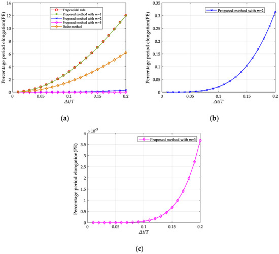
Figure 2. Percentage period elongation due to the proposed algorithm with m = 1,2,3: (a) Percentage period elongation with m = 1–3 comparing with that of trapezoidal rule and Bathe method. (b) Percentage period elongation with m = 2. (c) Percentage period elongation with m = 3.

4. A Feasible Scheme with Numerical Dissipation

To be sufficiently effective in solutions of structural dynamics, the time integration scheme should possess controllable numerical dissipation, such that the false vibration components of higher orders could be removed and the accuracy of results could be guaranteed. However, as discussed in Section 3, the integral scheme of Equation (15) does not have such numerical dissipation. In order to get over this difficulty, a feasible time integration scheme with numerical dissipation is proposed using the Galerkin weak form method. The detailed construction procedure is as follows.

Considering the Galerkin weak form shown in Equation (6) with linear time elements, let the trial function remain as the common interpolation of linear polynomials while the test function is as follows:

$${\tilde{v}}^h=N_{\alpha }{d}_v={\displaystyle \sum _{i=1}^2{N}_{\alpha i}(\zeta )v_i}$$

(30)

where $N_{\alpha }{}_i$ (i = 1,2) is the following constructed linear polynomial with a parameter ‘$\alpha$’ being introduced, i.e.,:

$$N_{\alpha }{}_1=-\frac{(\zeta -1-\alpha )}{2},N_{\alpha }{}_2=\frac{(\zeta +1-\alpha )}{2}.$$

(31)

That is to say, the test function in Equation (32) doesn’t satisfy the C₀ continuity between elements any more. Substituting such a trial function $u^h$ and test function ${\tilde{v}}^h$ into Equation (6), in consideration of the arbitrariness of $d_v$, the following solution formula for Equation (5) may be obtained:

$$K_{\alpha }d+\frac{2M}{\Delta t}(N{(1)}^T{\dot{u}}_{n+1}-N{(-1)}^T{\dot{u}}_n)=P_{\alpha }.$$

(32)

In Equation (32), there are many integration terms in both $K_{\alpha }$ and $P_{\alpha }$ which are also with respect to the parameter $\alpha$. Again, for the target to introduce numerical damping, the following integral formulae are used instead of the common Gauss integral in calculations of all the integral terms, i.e.,:

$${\displaystyle \underset{-1}{\overset{1}{\int }}f(\zeta )}\mathrm{d}\zeta =2f(\frac{\alpha }{2}).$$

(33)

Finally the following Newton-Raphson iterative scheme is yielded:

$$\begin{array}{c}(\frac{2}{\Delta t^2}M+\frac{1}{\Delta t}(1+\frac{\alpha }{2}){\overline{C}}_{\alpha /2}^{(k)}+\frac{1}{2}(1+\frac{\alpha }{2}{)}^2{\overline{K}}_{\alpha /2}^{(k)})u_{n+1}^{(k+1)}=(1+\frac{\alpha }{2})f_{\alpha /2}^{(k)}\\ +(\frac{2}{\Delta t^2}M+\frac{1}{\Delta t}(1+\frac{\alpha }{2}){\overline{C}}_{\alpha /2}^{(k)}-\frac{1}{2}(1-\frac{{\alpha }^2}{4}){\overline{K}}_{\alpha /2}^{(k)})u_n+\frac{2M}{\Delta t}{\dot{u}}_n\end{array}$$

(34)

$$\begin{array}{c}(-\frac{2}{\Delta t^2}M+\frac{1}{\Delta t}(1-\frac{\alpha }{2}){\overline{C}}_{\alpha /2}^{(k)}+\frac{1}{2}(1-\frac{{\alpha }^2}{4}){\overline{K}}_{\alpha /2}^{(k)})u_{n+1}^{(k+1)}+\frac{2M}{\Delta t}{\dot{u}}_{n+1}^{(k+1)}=\\ (1-\frac{\alpha }{2})f_{\alpha /2}^{(k)}+(-\frac{2}{\Delta t^2}M+\frac{1}{\Delta t}(1-\frac{\alpha }{2}){\overline{C}}_{\alpha /2}^{(k)}-\frac{1}{2}(1-\frac{\alpha }{2}{)}^2{\overline{K}}_{\alpha /2}^{(k)})u_n\end{array}$$

(35)

where

$${\overline{C}}_{\alpha /2}^{(k)}=\overline{C}({\dot{u}}_{{}_{\alpha /2}}^{(k)}),{\overline{K}}_{\alpha /2}^{(k)}=\overline{K}(u_{{}_{\alpha /2}}^{(k)}),f_{\alpha /2}^{(k)}=f(u_{{}_{\alpha /2}}^{(k)},{\dot{u}}_{{}_{\alpha /2}}^{(k)})$$

(36)

$$u_{{}_{\alpha /2}}^{(k)}=\frac{1}{2}(1-\frac{\alpha }{2})u_n^{}+\frac{1}{2}(1+\frac{\alpha }{2})u_{n+1}^{(k)}$$

(37)

$${\dot{u}}_{{}_{\alpha /2}}^{(k)}=-\frac{1}{2}{u}_n^{}+\frac{1}{2}{u}_{n+1}^{(k)}.$$

(38)

This is the proposed time integration scheme with numerical dissipation for linear time elements based on the Galerkin weak form.

Here, we give some analysis and verification of the introduced numerical dissipation. For the integration scheme shown in Equations (34)–(38), the transfer matrix $A$ is:

$$A=\frac{1}{{\alpha }^2{\mathsf{\Omega }}^2+4\alpha {\mathsf{\Omega }}^2+4{\mathsf{\Omega }}^2+16}\left[\begin{array}{cc}{\alpha }^2{\mathsf{\Omega }}^2-4{\mathsf{\Omega }}^2+16& 16\Delta t\\ -\frac{16{\mathsf{\Omega }}^2}{\Delta t}& {\alpha }^2{\mathsf{\Omega }}^2-4{\mathsf{\Omega }}^2+16\end{array}\right].$$

(39)

When $\alpha =0$, Equation (39) is the same as Equation (28), thus the scheme with a linear element in Equation (25) is a particular case of this improved scheme. The curves of the spectral radius obtained from A are shown in Figure 3 when $\alpha$ is set to be different values. From Figure 3, it can be seen that the spectral radius of the algorithm is unconditionally stable, and the numerical damping is easily controllable, since following an increase of $\alpha$ the numerical damping increases correspondingly. The curves of the spectral radius of the trapezoidal rule, Wilson $\theta$-method ($\theta = 1.4$) [41], and Bathe method ($\gamma =1/2$) [5] are shown in Figure 3 as well. The percentage of period elongation and amplitude decay are shown in Figure 4.

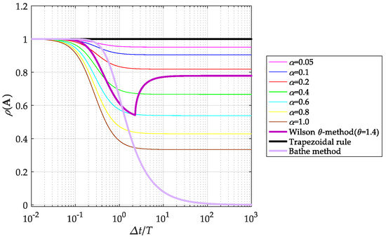
Figure 3. The spectral radii of transfer matrix A of the trapezoidal rule, Wilson θ-method, and Bathe method and the proposed scheme with different numerical damping.

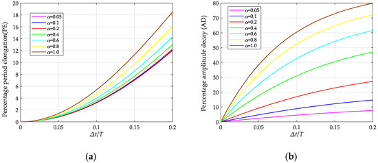
Figure 4. Percentage of period elongation and amplitude decay of the proposed scheme with numerical damping: (a) Percentage of period elongation. (b) Percentage of amplitude decay.

5. Numerical Examples

In this section, three representative numerical examples are given to show the efficiency of the proposed method. For each example, the results of the present method are compared with those of the following four algorithms: Tshe trapezoidal rule, Newmark method ($\gamma = 1/2, \beta = 1/6$) [1], Wilson $\theta$-method ($\theta = 1.4$) [41], and Bathe method ($\gamma = 1/2$) [5], which are commonly-used time integration algorithms in dynamics. All the results are obtained from the programming codes of MATLAB 2017a under the same computational circumstance.

5.1. The Simple Pendulum

The governing equation [43] for the nonlinear pendulum shown in Figure 5 is, $\ddot{u}+g/L\sin (u)=0$ with initial conditions $u(0)=\pi /2$ rad and $\dot{u}(0)=0$ rad/s, where $g$ is the gravitational acceleration, $L$ is the length of a massless suspension, and $u$ is the angle between the cycloid and vertical plane. The kinetic and potential energy of the system are $T_E=0.5L^2{\dot{u}}^2$ and $V_E=g(L-L\cos u)$, respectively. Moreover, the total energy is the sum of them. The solutions obtained from the trapezoidal rule with $\Delta t=0.0001$ s are approximately regarded as the exact solutions to evaluate the accuracy and efficiency of the present method here. This example aims to test the stability and accuracy of the proposed algorithm and the scheme without using numerical damping.

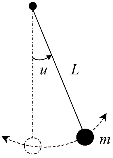
Figure 5. A simple pendulum.

Let $g/L=4{\pi }_{}^2{\mathrm{s}}^{-2}$ and take the time step to be $\Delta t = 0.15 \mathrm{s}$. The pendulum motion is calculated with the trapezoidal rule, Newmark method, Bathe method, Wilson $\theta$-method, and the proposed method. The displacement, velocity, and total energy histories from the trapezoidal rule are presented in Figure 6 and Figure 7, from which it can be seen that the results become considerably large when the time approaches 30 s, i.e., an unstable response is given from the trapezoidal rule for this example. The displacement responses of the exact solution and the other four methods are shown in Figure 8, which are all stable. It can be seen that, for Newmark method, the error of response gets bigger as the time goes on. For the Wilson method and Bathe method, noteworthy amplitude decay takes place in displacement responses since there is ineradicable numerical damping in these two methods, especially in the Wilson method. For this pendulum example, using methods without numerical damping may obtain more suitable responses, but there is no way for the Bathe method and Wilson method to control or remove the numerical damping, which will significantly affect the accuracy of the solution. The comparisons of energy responses shown in Figure 9 can further demonstrate the numerical dissipation property of the Wilson and Bathe methods. Both the displacement and velocity results of the present method with m = 2,3 are shown in Figure 10, which are stable and of high accuracy.

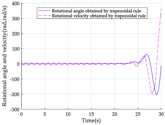
Figure 6. Responses of the pendulum using the trapezoidal rule with ∆t = 0.15 s.

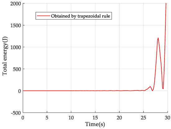
Figure 7. The energy evolution of the pendulum using the trapezoidal rule with ∆t = 0.15 s.

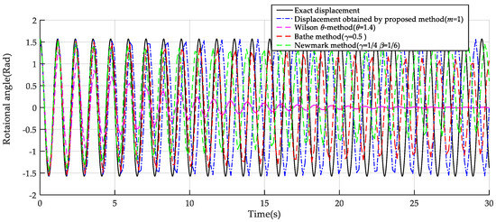
Figure 8. Comparisons of responses among the exact solution, Newmark method, Wilson method, Bathe method, and the present method with m = 1.

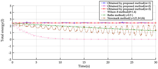
Figure 9. Comparisons of energy responses among the Newmark method, Wilson method, Bathe method, and the present method.

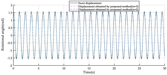
Figure 10. Displacement response of the present method with m = 2,3.

The error and convergence order of the present method are further studied. Let $g/L=3.438$ s⁻². The period of the response is approximately equal to 4 s. Taking the time step to be $\Delta t=0.2 \mathrm{s}$, $\Delta t=0.1 \mathrm{s}$, and $\Delta t=0.05 \mathrm{s}$ respectively, the accuracy of results of trapezoidal rule, Newmark method, Wilson $\theta$-method, Bathe method, and the present method with m = 1,2,3 are compared, with the following error estimates used:

$$\epsilon =\sqrt{{\displaystyle \sum _{i=1}^N{(\Vert u_i^h\Vert -\Vert u_i^{}\Vert )}^2}}/\sqrt{{\displaystyle \sum _{i=1}^N{(\Vert u_i^{}\Vert )}^2}}\times 100\%$$

(40)

where $u_i^h$ and $u_i^{}$ are the approximate displacement and the exact displacement at step i and $N$ is the total number of time steps. Error $\epsilon$ and convergence order $\rho$ from these seven schemes are given in Table 1 and Table 2, and the convergence curves are shown in Figure 11 correspondingly. The present algorithm with the linear element, quadratic element, and cubic element respectively, possess convergence orders of 2, 4 and 6 (i.e., 2 m) for both displacement and velocity, while all the other four methods are of a convergence order of 2. In this case, the accuracy of our method with m = 2,3 is obviously higher than that of others. For m = 1, the accuracy of the present algorithm is similar to that of the Newmark and Bathe methods, and is better than that of the Wilson $\theta$-method.

Table 1. Errors of displacement solutions (pendulum) calculated from different algorithms.

Algorithm	$\mathit{\epsilon }$$(\mathbf{\Delta }\mathit{t}=0.2 \mathbf{s})$	$\mathit{\epsilon }$$(\mathbf{\Delta }\mathit{t}=0.1 \mathbf{s})$	$\mathit{\epsilon }$$(\mathbf{\Delta }\mathit{t}=0.05 \mathbf{s})$	$\mathit{\rho }$
Trapezoidal rule	1.81e+00	5.00e−01	1.29e−01	2
Bathe method ($\gamma =1/2$)	1.33e+00	3.45e−01	8.77e−02	2
Wilson $\theta$-method ($\theta =1.4$)	5.11e+00	1.41e+00	3.71e−01	2
Newmark method ($\gamma =1/2,\beta =1/6$)	1.17e+00	3.36e−01	8.73e−02	2
Present algorithm with m = 1	1.37e+00	3.49e−01	8.81e−02	2
Present algorithm with m = 2	5.29e−03	3.31e−04	2.08e−05	4
Present algorithm with m = 3	1.93e−05	3.10e−07	4.75e−09	6

Table 2. Errors of velocity solutions (pendulum) calculated from different algorithms.

Algorithm	$\mathit{\epsilon }$$(\mathbf{\Delta }\mathit{t}=0.2 \mathbf{s})$	$\mathit{\epsilon }$$(\mathbf{\Delta }\mathit{t}=0.1 \mathbf{s})$	$\mathit{\epsilon }$$(\mathbf{\Delta }\mathit{t}=0.05 \mathbf{s})$	$\mathit{\rho }$
Trapezoidal rule	1.82e+00	5.27e−01	1.38e−01	2
Bathe method ($\gamma =1/2$)	1.50e+00	3.72e−01	9.34e−02	2
Wilson $\theta$-method ($\theta =1.4$)	5.45e+00	1.54e+00	4.08e−01	2
Newmark method ($\gamma =1/2,\beta =1/6$)	1.42e+00	3.88e−01	9.84e−02	2
Present algorithm with m = 1	1.62e+00	3.94e−01	9.74e−02	2
Present algorithm with m = 2	3.81e−03	2.36e−04	1.46e−05	4
Present algorithm with m = 3	1.24e−05	1.90e−07	1.34e−09	6

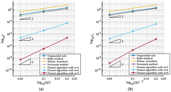
Figure 11. Convergence curves of displacements and velocities of the seven integration schemes: (a) Displacement/rotational angle. (b) Velocity.

5.2. Long Span Planar Skeletal Structure

A large span truss model [44] with a length of 25 m and the height of 1m is shown in Figure 12. The elastic modulus is E = 2.0 × 10⁵ MPa, the density is 7800 kg/m³, and the cross-section area of each bar is 100 mm². In FEM, the large displacement Saint Venant Kirchhoff material model and complete Lagrange description [45] are adopted for the truss elements. There are 101 member bars in total, and each member bar is a single element with hinged constraints at both ends. As shown in Figure 9, Points A and B are located near the middle of the span and are set to gain an initial velocity v = 100 m/s. This example is used to test both the numerical stability and numerical dissipation of the algorithm, and the integration scheme in Equations (34)–(38) with $\alpha \ge 0$.

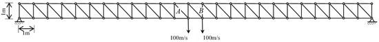
Figure 12. Long span planar skeletal structure.

Firstly, setting the time step $\Delta t=0.01 \mathrm{s}$, this problem was solved with trapezoidal rule and the proposed method with $\alpha =0$. The vertical responses at Point A are shown in Figure 13. It can be obviously seen that after about 2 s, the numerical errors of the acceleration start to accumulate significantly for the trapezoidal rule, while the proposed method with $\alpha =0$ still performs well. Enlarging the time step size to be $\Delta t=0.02 \mathrm{s}$ and $\Delta t=0.04 \mathrm{s}$, the responses resulted from the proposed method with $\alpha =0$ remain stable, as shown in Figure 14, i.e., the proposed method performs better in numerical stability than the trapezoidal rule for this example.

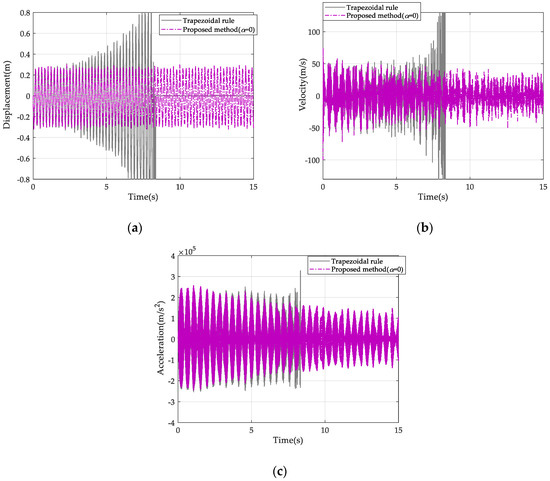
Figure 13. Vertical response of Point A with the trapezoidal rule and the proposed method when ∆t = 0.01 s: (a) Displacement response. (b) Velocity response. (c) Acceleration response.

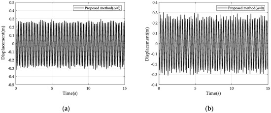
Figure 14. Vertical displacement responses of Point A with ∆t = 0.02 s and ∆t = 0.04 s: (a) Displacement response with ∆t = 0.02 s. (b) Displacement response with ∆t = 0.04 s.

Secondly, in order to verify the efficiency in numerical dissipation of the proposed algorithm, we set the time step interval $\Delta t=0.001 \mathrm{s}$ and solve the problem with $\alpha =0,0.01,0.05,0.1,0.2$ respectively, the resulting responses are shown in Figure 15 and Figure 16. It can be seen that, when $\alpha =0$, the high-frequency oscillation of the system is very intense. With an increase of $\alpha$, i.e., numerical damping is introduced, the high-order-frequency response of the system obviously decays. The higher $\alpha$ is, the faster the high frequency response decays. In addition, the low frequency response remains intact while no obvious amplitude decay and no period elongation appear. Therefore, the proposed method can effectively filter out the high frequency response of the system while retaining the low frequency response well through the controllable numerical damping.

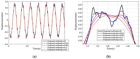
Figure 15. Vertical displacement responses of Point A with ∆t = 0.001 s: (a) Displacement responses. (b) Partial enlarged drawing of displacement responses.

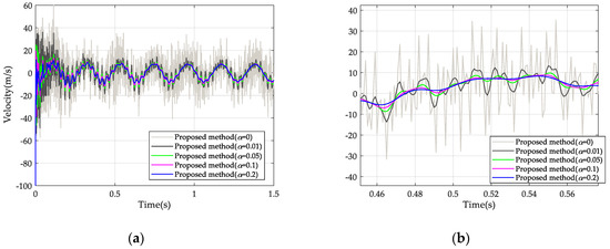
Figure 16. Vertical velocity responses of Point A with ∆t = 0.001 s: (a) Velocity responses. (b) Partial enlarged drawing of velocity responses.

Thirdly, the vertical displacement responses at Point A calculated with the Wilson $\theta$-method, Bathe method, and the proposed method are shown and compared in Figure 17 and Figure 18, where $\Delta t=0.01 \mathrm{s}$ and the computational times are correspondingly listed in Table 3. It is found that, for the Wilson method the computational time is short, but the numerical damping is a little large, which results in excessive dissipation of low frequency modes and significant amplitude decay. For Bathe method, the low frequency modes are retained well and the high frequency modes of the response are quickly filtered out, but the computational time is longer. Nevertheless, with the setting of different α, the present method performs better than the Wilson method in numerical dissipation and better than Bathe method in computational efficiency.

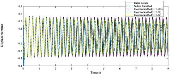
Figure 17. Vertical displacement responses of Point A with the Wilson method, Bathe method, and the proposed method when ∆t = 0.01 s.

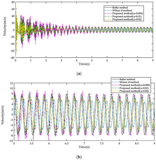
Figure 18. Velocity responses of Point A with the Wilson method, Bathe method, and the proposed method when ∆t = 0.01 s: (a) Global velocity responses. (b) Partial enlarged drawing of velocity responses.

Table 3. Computational time of different methods.

Method	Computational Time (s)
Bathe method ($\gamma =1/2$)	16.34
Wilson $\theta$-method ($\theta =1.4$)	9.29
Proposed method ($\alpha =0.005$)	9.83
Proposed method ($\alpha =0.01$)	9.48
Proposed method ($\alpha =0.02$)	9.33

5.3. Cantilever Beam

Consider the cantilever Euler-Bernoulli beam under a uniformly distributed pulse load as the example [5], which is shown in Figure 19. A linear elastic constitutive relation and degenerate Green–Lagrange strain tensor [45] are adopted to describe the finite elements, and 400 elements are used in spatial discretization. Linear Lagrange element interpolation is used for axial displacement, and cubic Hermite element interpolation is used for lateral and rotational displacements.

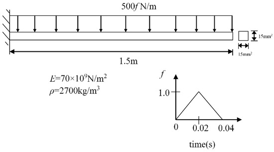
Figure 19. Cantilever beam model.

Letting $\Delta t=0.002 \mathrm{s}$, the results of vibration displacement, velocity, and acceleration at the free end of the beam are shown in (Figure 20, Figure 21 and Figure 22), calculated from trapezoidal rule, Bathe method, Wilson θ-method and the proposed method with α = 0.02, respectively. The trapezoidal rule again shows unstable performance. The Bathe method, Wilson θ-method, and the proposed method all give stable responses. Both the Bathe method and the proposed method perform well, however, for the Wilson θ-method, acceleration decays as time goes on and the numerical dissipation of the global response is a little larger, as shown in Figure 22c.

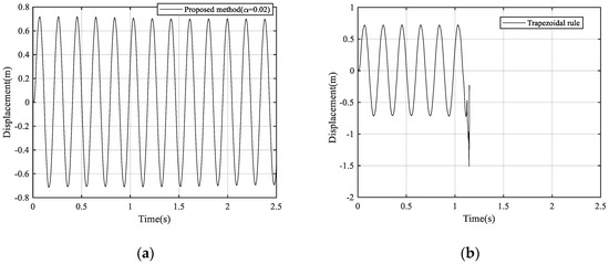
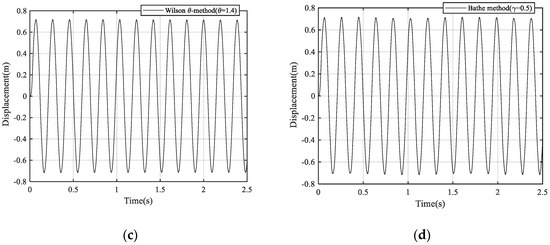
Figure 20. The displacement responses at the free end of the cantilever beam: (a) Using the proposed method, (b) using the trapezoidal rule, (c) using Wilson θ-method, and (d) using Bathe method.

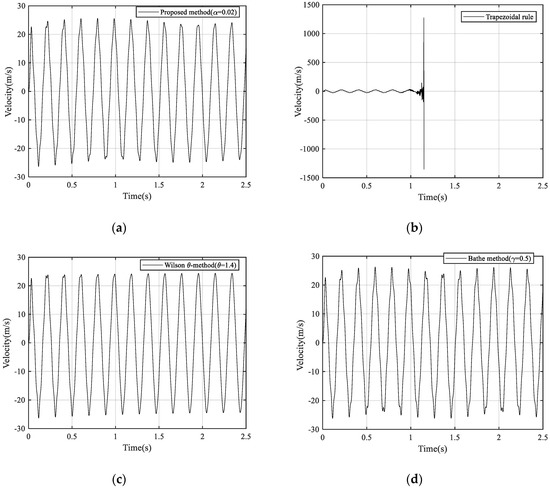
Figure 21. The velocity responses at the free end of the cantilever beam: (a) Using the proposed method, (b) using the trapezoidal rule, (c) using Wilson θ-method, and (d) using Bathe method.

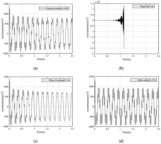
Figure 22. The acceleration responses at the free end of the cantilever beam: (a) Using the proposed method, (b) using the trapezoidal rule, (c) using Wilson θ-method, and (d) using Bathe method.

Solving the beam with different numbers of spatial elements, the corresponding computational time taken in each method is listed in Table 4, and then the variation of computational time versus the number of degrees of freedom (DOFs) is plotted in Figure 23. The computational speed of the proposed method is as good as the Wilson method and is obviously better than the Bathe method.

Table 4. Computational times of different methods (s).

Method\No. of DOFs	150	300	450	600	750	900	1050	1200
Bathe method	90.49	196.38	300.34	456.37	656.15	894.85	1249.68	1759.70
Wilson θ-method	53.67	108.31	175.25	281.07	373.99	511.82	696.59	896.19
This algorithm (α = 0.02)	54.73	107.77	188.43	294.14	417.34	530.81	717.74	935.43

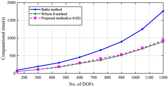
Figure 23. Variation of computational time versus the number of degrees of freedom (DOFs) of the model.

6. Conclusions

Taking the nonlinear dynamic Equation (1) as the model problem, a step-by-step time integration method is proposed based on the Galerkin finite element approximation and Newton–Raphson iteration. In summary, the following four conclusions of this method should be noted:

• For the proposed method based on the Galerkin FEM, usually time elements of degree m = 1,2,3 are used in practical computation. Numerical examples show that such elements can gain a convergence order of 2m for both displacement and velocity results.
• When a reduced Gauss integral method is applied in computation, the present method is unconditional stability.
• For linear elements, a feasible time integration scheme with controllable numerical damping has been constructed by modifying the test function and introducing a special integral rule.
• This is a self-starting and one-step method, which can effectively solve both linear and nonlinear structural dynamic problems. Representative numerical examples have shown its reliability and efficiency, and according to comparisons of results with the trapezoidal rule, Wilson θ-method, and Bathe method, the present method performs well in stability with controllable numerical dissipation, and its computational efficiency turns out to be superior as well.

The proposed time integration method is of comprehensive capabilities in nonlinear dynamics. Furthermore, since it originates from FEM, self-adaptive FE techniques can be directly introduced into it, and then an adaptive integration algorithm can be established with the size of time step being automatically produced, leading to more efficient solutions of nonlinear dynamic problems.

References

- Newmark, N.M. A method of computation for structural dynamics. J. Eng. Mech. Div. 1959, 85, 67–94. [Google Scholar]
- Simo, J.C.; Tarnow, N.; Wong, K.K. Exact energy-momentum conserving algorithms and symplectic schemes for nonlinear dynamics. Comput. Methods Appl. Mech. Eng. 1992, 100, 63–116. [Google Scholar] [CrossRef]
- Kuhl, D.; Crisfield, M.A. Energy-conserving and decaying Algorithms in non-linear structural dynamics. Numer. Methods Eng. 1999, 45, 569–599. [Google Scholar] [CrossRef]
- Hughes, R. The Finite Element Method: Linear Static and Dynamic Finite Element Analysis. Religion 2003, 6, 222. [Google Scholar]
- Bathe, K.J.; Baig, M.M. On a composite implicit time integration procedure for nonlinear dynamics. Comput. Struct. 2005, 83, 2513–2524. [Google Scholar] [CrossRef]
- Hilber, H.M.; Hughes, T.J.R.; Taylor, R.L. Improved Numerical Dissipation for Time Integration Algorithms in Structural Dynamics. Earthq. Eng. Struct. Dyn. 1977, 5, 283–292. [Google Scholar] [CrossRef]
- Chung, J.; Hulbert, G.M. A Time Integration Algorithm for Structural Dynamics with Improved Numerical Dissipation: The Generalized-α Method. J. Appl. Mech. 1993, 60, 371. [Google Scholar] [CrossRef]
- Hughes, T.J.R.; Caughey, T.K.; Liu, W.K. Finite-element methods for nonlinear elastodynamics which conserve energy. ASME J. Appl. Mech. 1978, 45, 366–370. [Google Scholar] [CrossRef]
- Kuhl, D.; Ramm, E. Constraint Energy Momentum Algorithm and its application to non-linear dynamics of shells. Comput. Methods Appl. Mech. Eng. 1996, 136, 293–315. [Google Scholar] [CrossRef]
- Liu, T.; Zhao, C.; Li, Q.; Zhang, L. An efficient backward Euler time-integration method for nonlinear dynamic analysis of structures. Comput. Struct. 2012, 106, 20–28. [Google Scholar] [CrossRef]
- Simo, J.C.; Tarnow, N. Conserving algorithms for nonlinear dynamics. In New Methods in Transient Analysis, The Winter Annual Meeting of the American Society of Mechanical Engineers Anaheim, CA; Smolinski, P., Liu, W.K., Hulbert, G., Tamma, K., Eds.; The American Society of Mechanical Engineers: New York, NY, USA, 1992. [Google Scholar]
- Criseld, M.A.; Shi, J. A co-rotational element time-integration strategy for non-linear dynamics. Int. J. Numer. Methods Eng. 1994, 37, 1897–1913. [Google Scholar] [CrossRef]
- Simo, J.C.; Wong, K.K. Unconditionally stable algorithms for rigid body dynamics that exactly preserve energy and momentum. Int. J. Numer. Methods Eng. 1991, 31, 19–52. [Google Scholar] [CrossRef]
- Criseld, M.A.; Shi, J. An energy conserving co-rotational procedure for non-linear dynamics with finite elements. Nonlinear Dyn. 1996, 9, 37–52. [Google Scholar] [CrossRef]
- Simo, J.C.; Tarnow, N.; Doblare, M. Non-linear dynamics of three-dimensional rods: Exact energy and momentum conserving algorithms. Int. J. Numer. Methods Eng. 1995, 38, 1431–1473. [Google Scholar] [CrossRef]
- Xing, Y.; Qin, M.; Guo, J. A time finite element method based on the differential quadrature rule and hamilton’s variational principle. Appl. Sci. 2017, 7, 138. [Google Scholar] [CrossRef]
- Gurtin, M.E. Variational principles for linear initial-value problems. Q. Appl. Math. 1964, 22, 252–256. [Google Scholar] [CrossRef]
- Gurtin, M.E. Variational principles for linear elastodynamics. Arch. Ration. Mech. Anal. 1964, 16, 34–50. [Google Scholar] [CrossRef]
- Fried, I. Finite-element analysis of time-dependent phenomena. AIAA J. 1969, 7, 1170–1173. [Google Scholar] [CrossRef]
- Argyris, J.H.; Scharpf, D.W. Finite elements in time and space. Aeronaut. J. 1969, 73, 1041–1044. [Google Scholar] [CrossRef]
- Oden, J.T. A general theory of finite elements. II. Applications. Int. J. Numer. Methods Eng. 1969, 1, 247–259. [Google Scholar] [CrossRef]
- Bailey, C.D. Application of Hamilton’s law of varying action. AIAA J. 1975, 13, 1154–1157. [Google Scholar] [CrossRef]
- Bailey, C.D. The method of Ritz applied to the equation of Hamilton. Comput. Methods Appl. Mech. Eng. 1976, 7, 235–247. [Google Scholar] [CrossRef]
- Simkins, T.E. Finite elements for initial value problems in dynamics. AIAA J. 1981, 19, 1357–1362. [Google Scholar] [CrossRef]
- Borri, M.; Ghiringhelli, G.L.; Lanz, M.; Mantegazza, P.; Merlini, T. Dynamic response of mechanical systems by a weak Hamiltonian formulation. Comput. Struct. 1985, 20, 495–508. [Google Scholar] [CrossRef]
- Krishna, M.S.; Manjeet, S.K. Three and four step least square finite element schemes in the time domain. Commun. Numer. Methods Eng. 1996, 12, 425–432. [Google Scholar]
- Kawahara, M.; Hasegawa, K. Periodic galerkin finite element method of tidal flow. Int. J. Numer. Methods Eng. 1978, 12, 115–128. [Google Scholar] [CrossRef]
- Jia, Z.; Cheng, X.; Zhao, M. A new method for roots of monic quaternionic quadratic polynomial. Comput. Math. Appl. 2009, 9, 1852–1859. [Google Scholar] [CrossRef]
- Hoff, C.; Hughes, T.J.R.; Hulbert, G.; Pahl, P.J. Extended comparison of the hilber-hughes-taylor α-method and the θ1-method. Comput. Methods Appl. Mech. Eng. 1989, 76, 87–94. [Google Scholar] [CrossRef]
- Chang, J.C. Combining genetic algorithm and taylor series expansion approach for doa estimation in space-time cdma systems. Appl. Soft Comput. J. 2015, 28, 208–217. [Google Scholar] [CrossRef]
- Zienkiewicz, O.C.; Wood, W.L.; Hine, N.W.; Taylor, R.L. A unified set of single step algorithms. Part 1: General formulation and applications. Int. J. Numer. Methods Eng. 1984, 20, 1529–1553. [Google Scholar] [CrossRef]
- Khan, I.R.; Ohba, R.; Hozumi, N. Mathematical proof of closed form expressions for finite difference approximations based on taylor series. J. Comput. Appl. Math. 2003, 150, 303–310. [Google Scholar] [CrossRef]
- Zienkiewicz, O.C. A new look at the Newmark, Houbolt and other time stepping formulas. A weighted residual approach. Earthq. Eng. Struct. Dyn. 1977, 5, 413–418. [Google Scholar] [CrossRef]
- Xing, X.; Zhang, X. A time integration method based on the weak form Galerkin method. Eng. Mech. 2006, 23, 8–12. (In Chinese) [Google Scholar]
- Hoff, C.; Pahl, P.J. Practical performance of the θ1-method and comparison with other dissipative algorithms in structural dynamics. Comput. Methods Appl. Mech. Eng. 1988, 67, 87–111. [Google Scholar] [CrossRef]
- Betsch, P.; Steinmann, P. Inherently Energy Conserving Time Finite Elements for Classical Mechanics. J. Comput. Phys. 2000, 160, 88–116. [Google Scholar] [CrossRef]
- Betsch, P.; Steinmann, P. Conservation properties of a time FE method—Part II: Time-stepping schemes for non-linear elastodynamics. Int. J. Numer. Methods Eng. 2001, 50, 1931–1955. [Google Scholar] [CrossRef]
- Reed, W.H.; Hill, T.R. Triangular Mesh Methods for the Neutron Transport Equation; Los Alamos Scientific Laboratory: Los Alamos, NM, USA, 1973. [Google Scholar]
- Lasaint, P.; Raviart, P.A. On a finite element method for solving the neutron transport equation. In Mathematical Aspects of Finite Elements in Partial Differential Equations; de Boor, C., Ed.; Academic Press: New York, NY, USA, 1974; pp. 89–123. [Google Scholar]
- Bauchau, O.A.; Theron, N.J. Energy decaying scheme for non-linear beam models. Comput. Methods Appl. Mech. Eng. 1996, 134, 37–56. [Google Scholar] [CrossRef]
- Wilson, E.L.; Farhoomand, I.; Bathe, K.J. Nonlinear dynamic analysis of complex structures. Int. J. Earthq. Eng. Struct. Dyn. 1973, 1, 241–252. [Google Scholar] [CrossRef]
- Xing, Q.; Yang, X. An EEP adaptive strategy of the Galerkin FEM for dynamic equations of discrete systems. Appl. Math. Mech. 2017, 38, 133–143. [Google Scholar]
- Li, J.; Yu, K.; Li, X. A novel family of controllably dissipative composite integration algorithms for structural dynamic analysis. Nonlinear Dyn. 2019, 96, 2475–2507. [Google Scholar] [CrossRef]
- Pan, T.; Wu, B.; Guo, L.; Shen, Y. Application of energy conserving step-by-step integration algorithm in dynamic analysis of engineering structures. Eng. Mech. 2014, 31, 21–27. [Google Scholar]
- De Borst, R.; Crisfield, M.A.; Remmers, J.J.C.; Clemens, V.V. Nonlinear Finite Element Analysis of Solids and Structures; John Wiley & Sons: New York, NY, USA, 2012. [Google Scholar]
© 2019 by the authors. Licensee MDPI, Basel, Switzerland. This article is an open access article distributed under the terms and conditions of the Creative Commons Attribution (CC BY) license (http://creativecommons.org/licenses/by/4.0/).