Assessment of Turbulence Modelling in the Wake of an Actuator Disk with a Decaying Turbulence Inflow


Abstract
1. Introduction
2. Homogeneous Turbulence
3. Experimental Setup and Measurement Campaigns
4. Model Description
4.1. Numerical Model
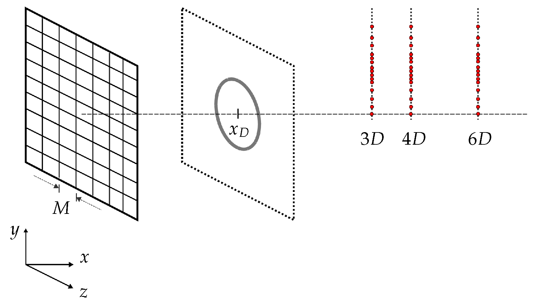
4.2. Computational Domain and Grid Resolution
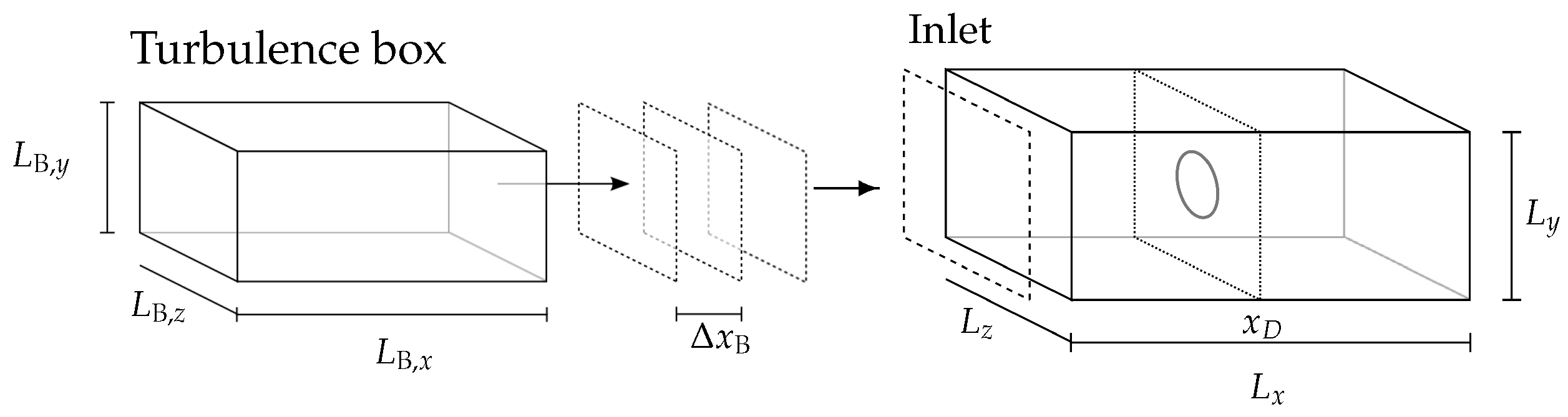
4.3. Generation of Turbulent Inflow, Introduction into the Computational Domain and Boundary Conditions
4.4. Estimation of Integral Lengthscales
4.5. Actuator Disk Model
4.6. About RANS Results
5. Results and Discussion
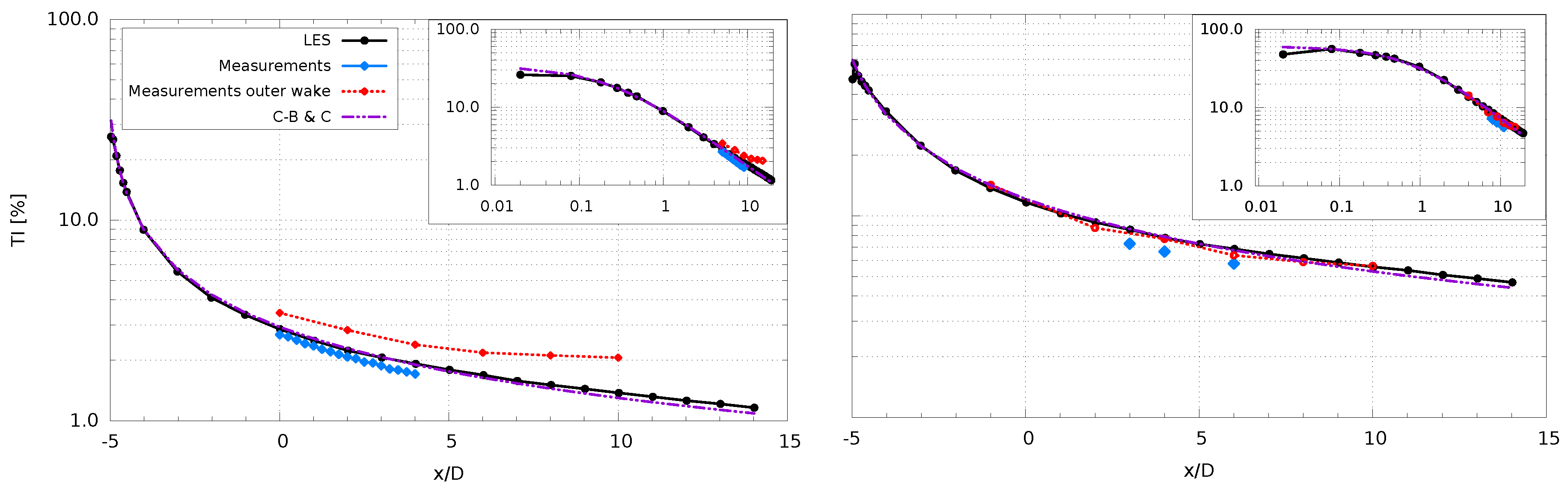
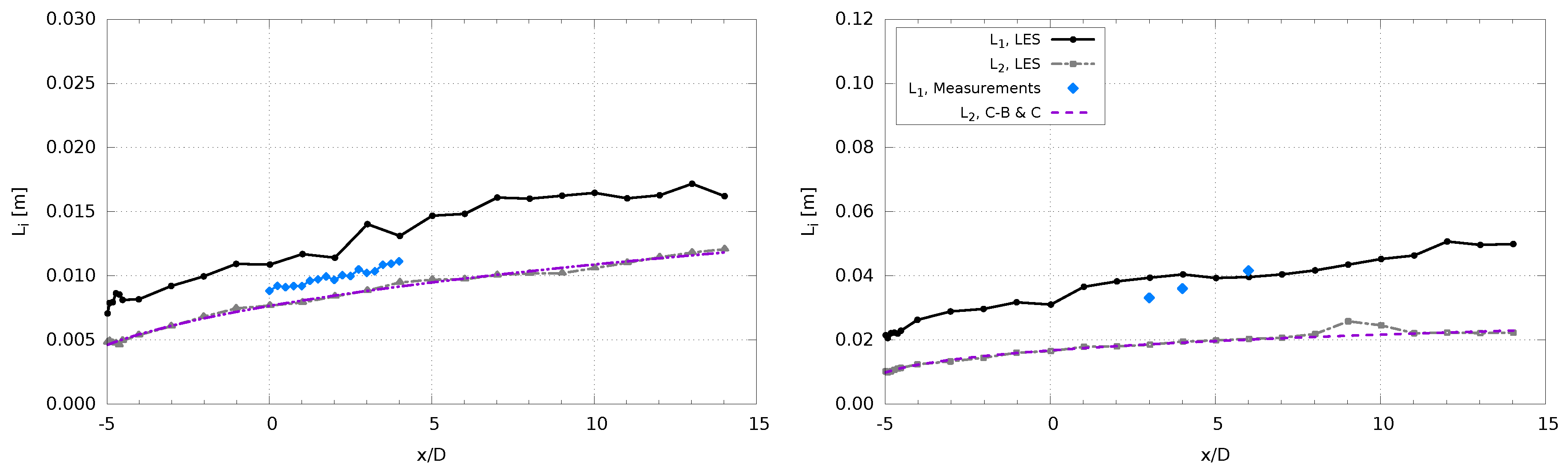
5.1. Turbulence Decay and Integral Lengthscale Development without Disk
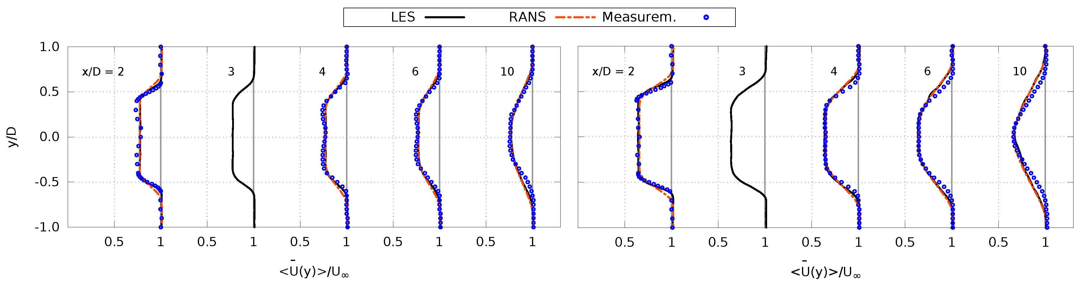
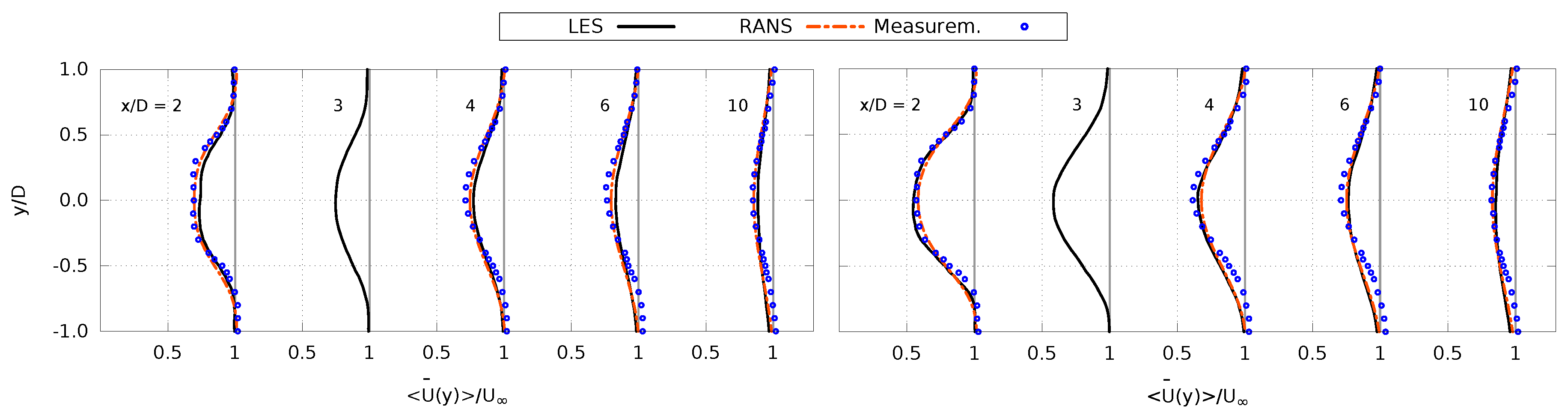
5.2. Velocity Deficit
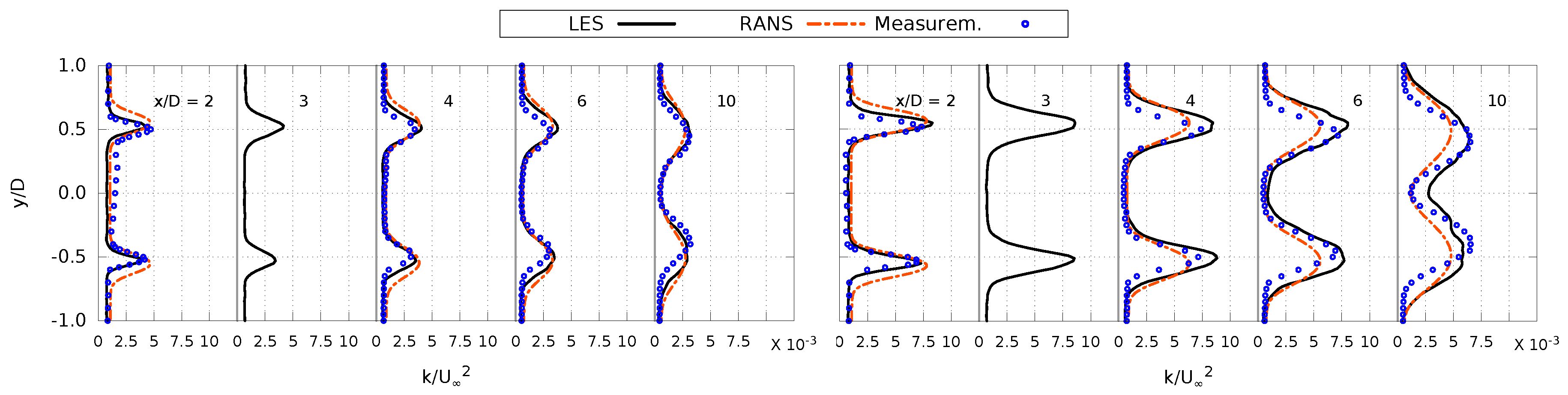
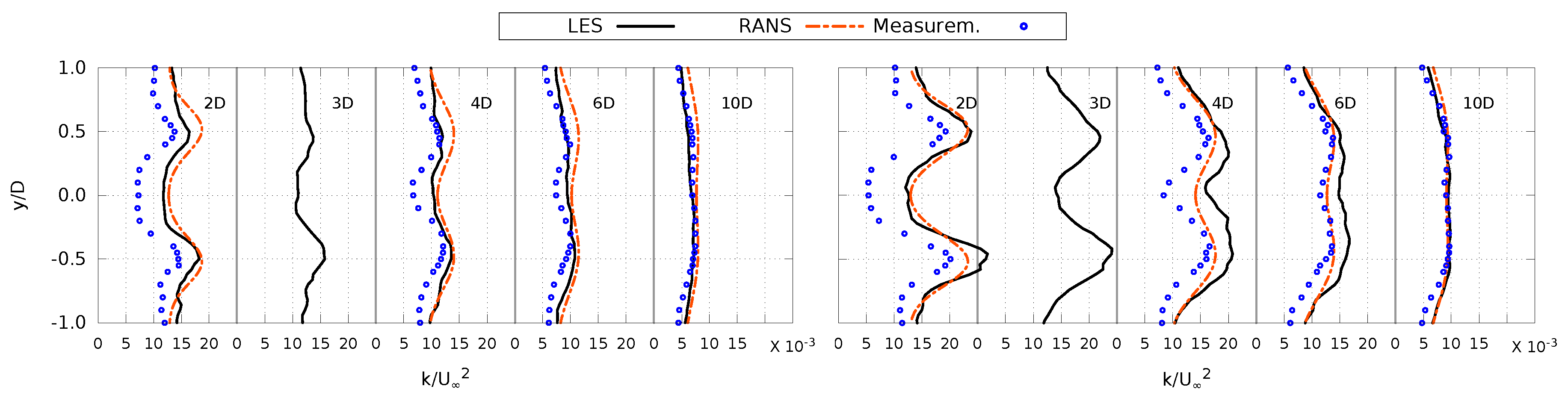
5.3. Turbulence Kinetic Energy in the Wake
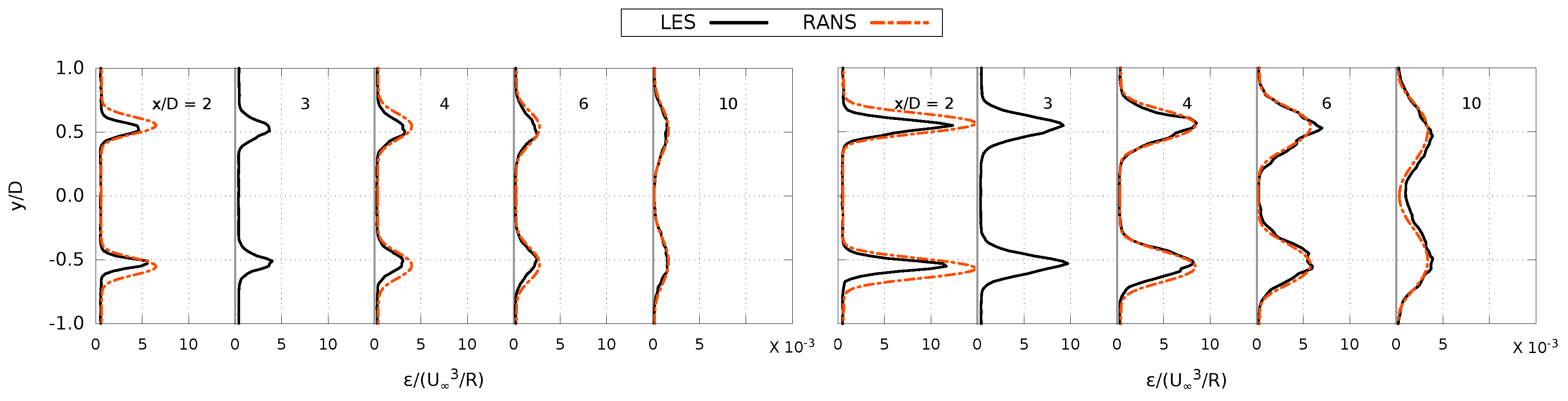
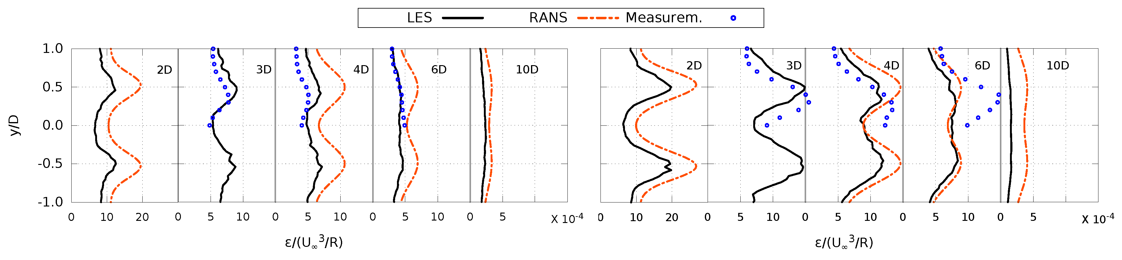
5.4. Turbulence Dissipation in the Wake
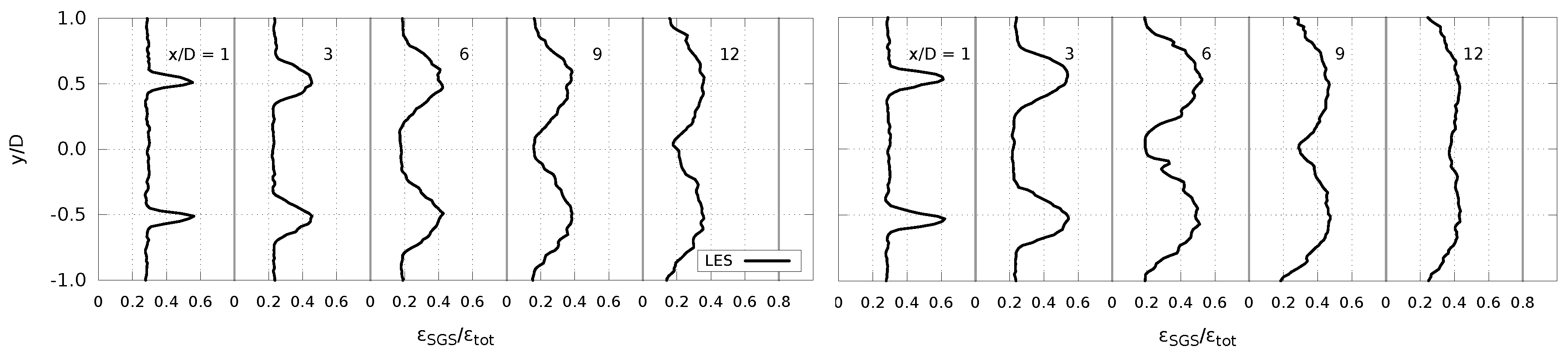
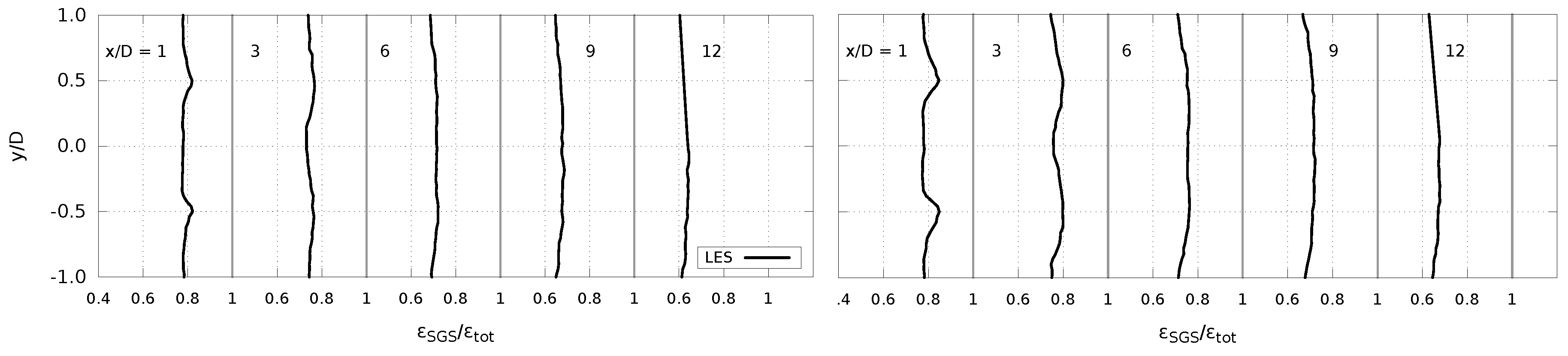
5.5. LES Modelling in the Wake
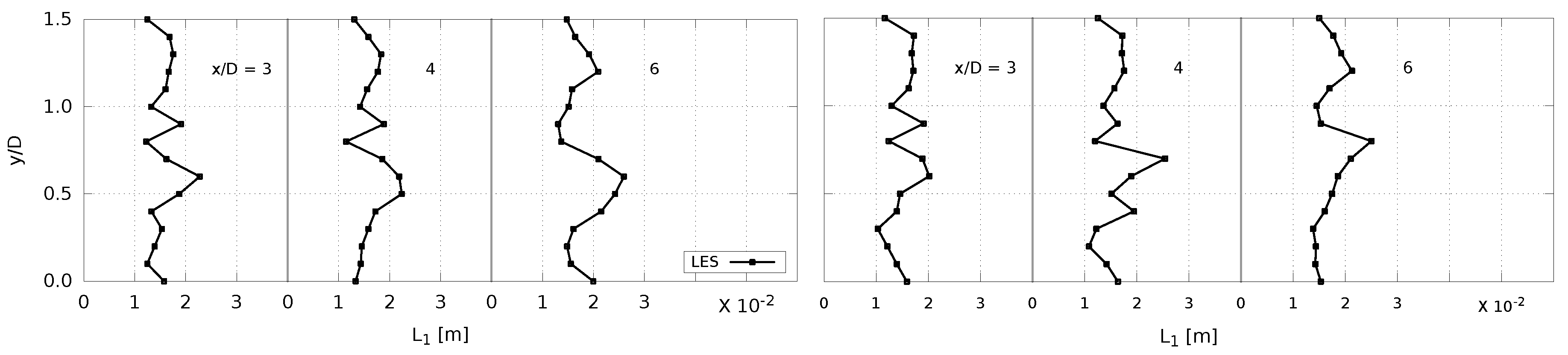
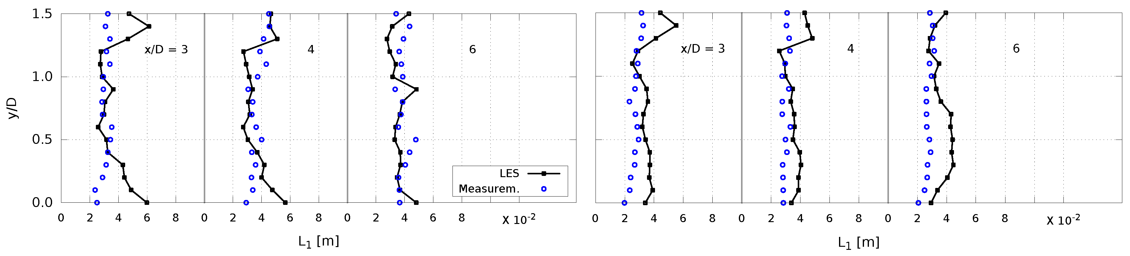
5.6. Integral Lengthscale in the Wake
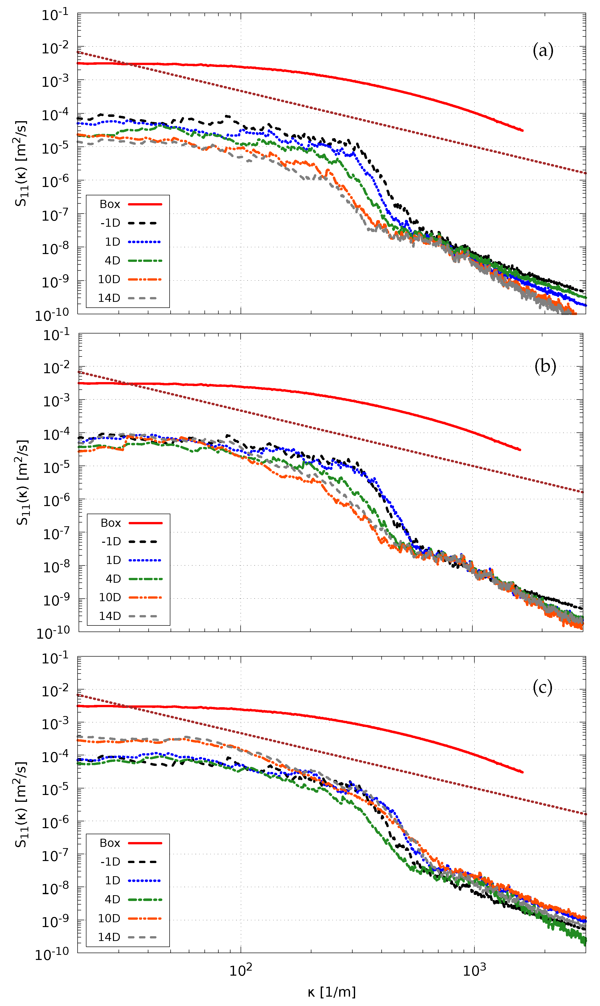
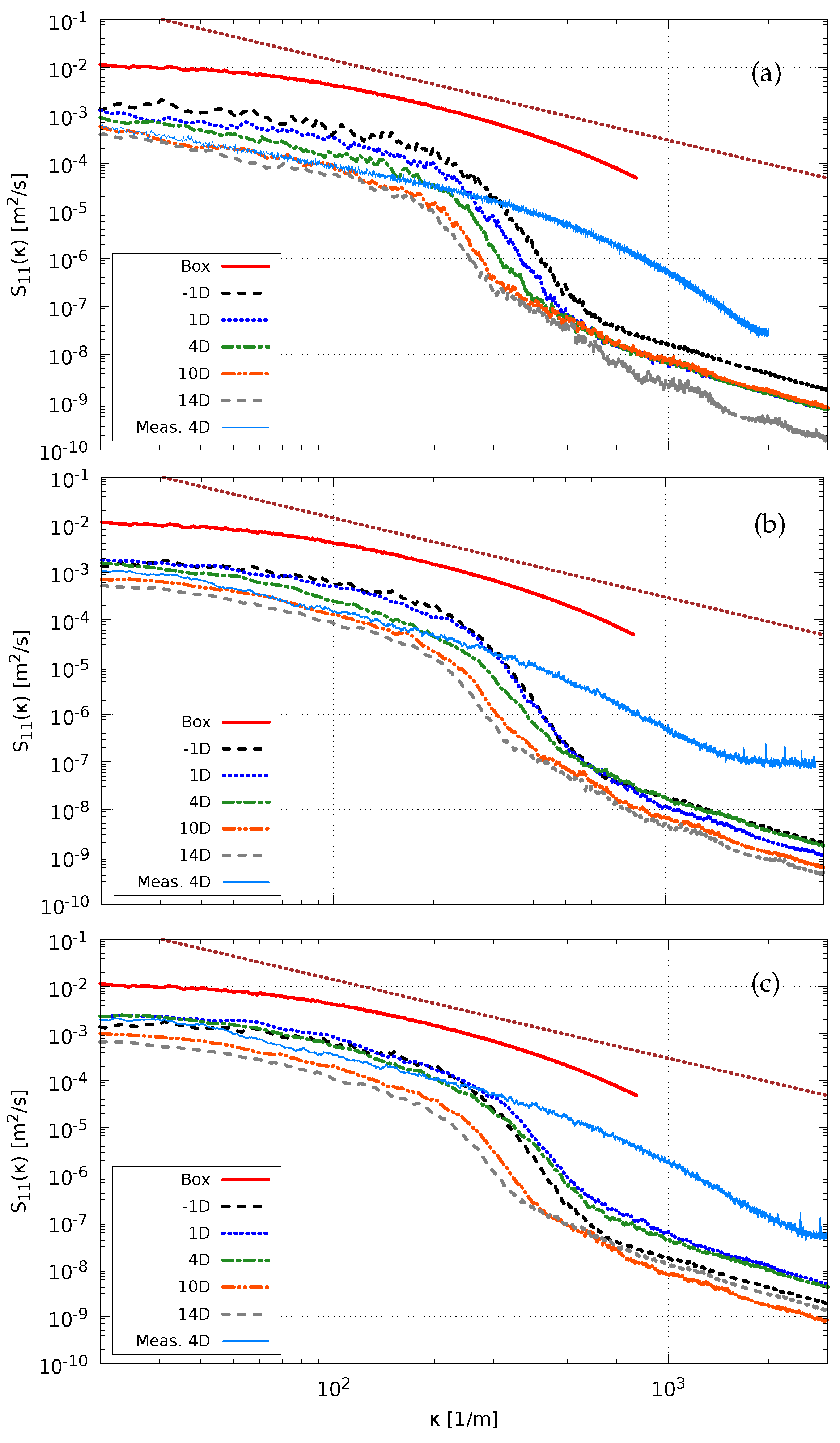
5.7. Spectra behind Disks
5.8. Vorticity Contours
6. Summary and Conclusions
- The evolution of was not noticeably different in the wake in comparison to what was observed in the decaying homogeneous turbulence.
- Turbulence scales in the wake appear to be dominated by the inflow characteristics and this effect increases with the level of TI in the inflow.
- It is seen that the resolved/subgrid modelling ratio in the freestream flow prevails in the wake in relation to the increasing level of ambient turbulence.
Author Contributions
Funding
Acknowledgments
Conflicts of Interest
References
- Crespo, A.; Hernandez, J.; Frandsen, S. Survey of modelling methods for wind turbine wakes and wind farms. Wind Energy 1999, 2, 1–24. [Google Scholar] [CrossRef]
- Calaf, M.; Meneveau, C.; Meyers, J. Large eddy simulation study of fully developed wind-turbine array boundary layers. Phys. Fluids 2010, 22, 015110. [Google Scholar] [CrossRef]
- Churchfield, M.J.; Lee, S.; Moriarty, P.J.; Martinez, L.A.; Leonardi, S.; Vijayakumar, G.; Brasseur, J.G. A large-eddy simulation of wind-plant aerodynamics. In Proceedings of the 50th AIAA Aerospace Sciences Meeting Including the New Horizons Forum and Aerospace Exposition, Nashville, TN, USA, 9–12 January 2012; p. 537. [Google Scholar]
- Nilsson, K.; Ivanell, S.; Hansen, K.S.; Mikkelsen, R.; Sørensen, J.N.; Breton, S.P.; Henningson, D. Large-eddy simulations of the Lillgrund wind farm. Wind Energy 2015, 18, 449–467. [Google Scholar] [CrossRef]
- Troldborg, N. Actuator Line Modeling of Wind Turbine Wakes. Ph.D. Thesis, Technical University of Denmark, Lyngby, Denmark, 2008. [Google Scholar]
- Ivanell, S.A. Numerical Computations of Wind Turbine Wakes. Ph.D. Thesis, Royal Institute of Technology, Stockholm, Sweden, 2009. [Google Scholar]
- Chamorro, L.P.; Porté-Agel, F. A wind-tunnel investigation of wind-turbine wakes: Bundary-layer turbulence effects. Bound.-Layer Meteorol. 2009, 132, 129–149. [Google Scholar] [CrossRef]
- Porté-Agel, F.; Wu, Y.T.; Lu, H.; Conzemius, R.J. Large-eddy simulation of atmospheric boundary layer flow through wind turbines and wind farms. J. Wind Eng. Ind. Aerodyn. 2011, 99, 154–168. [Google Scholar] [CrossRef]
- Sørensen, J.N.; Myken, A. Unsteady actuator disc model for horizontal axis wind turbines. J. Wind Eng. Ind. Aerodyn. 1992, 39, 139–149. [Google Scholar] [CrossRef]
- Ammara, I.; Leclerc, C.; Masson, C. A viscous three-dimensional differential/actuator-disk method for the aerodynamic analysis of wind farms. J. Sol. Energy Eng. 2002, 124, 345–356. [Google Scholar] [CrossRef]
- Jiménez, A.; Crespo, A.; Migoya, E.; Garcia, J. Large-eddy simulation of spectral coherence in a wind turbine wake. Environ. Res. Lett. 2008, 3, 015004. [Google Scholar] [CrossRef]
- Aubrun, S.; Loyer, S.; Hancock, P.; Hayden, P. Wind turbine wake properties: Comparison between a non-rotating simplified wind turbine model and a rotating model. J. Wind Eng. Ind. Aerodyn. 2013, 120, 1–8. [Google Scholar] [CrossRef]
- Aubrun, S.; Devinant, P.; Espana, G. Physical modelling of the far wake from wind turbines. Application to wind turbine interactions. In Proceedings of the European Wind Energy Conference, Milan, Italy, 7–10 May 2007; pp. 7–10. [Google Scholar]
- Espana, G.; Aubrun, S.; Loyer, S.; Devinant, P. Spatial study of the wake meandering using modelled wind turbines in a wind tunnel. Wind Energy 2011, 14, 923–937. [Google Scholar] [CrossRef]
- Espana, G.; Aubrun, S.; Loyer, S.; Devinant, P. Wind tunnel study of the wake meandering downstream of a modelled wind turbine as an effect of large scale turbulent eddies. J. Wind Eng. Ind. Aerodyn. 2012, 101, 24–33. [Google Scholar] [CrossRef]
- Thacker, A.; Loyer, S.; Aubrun, S. Comparison of turbulence length scales assessed with three measurement systems in increasingly complex turbulent flows. Exp. Therm. Fluid Sci. 2010, 34, 638–645. [Google Scholar] [CrossRef]
- Sumner, J.; Espana, G.; Masson, C.; Aubrun, S. Evaluation of RANS/actuator disk modelling of wind turbine wake flow using wind tunnel measurements. Int. J. Eng. Syst. Model. Simul. 2013, 5, 147–158. [Google Scholar] [CrossRef]
- Tabor, G.R.; Baba-Ahmadi, M. Inlet conditions for large eddy simulation: a review. Comput. Fluids 2010, 39, 553–567. [Google Scholar] [CrossRef]
- Lund, T.S.; Wu, X.; Squires, K.D. Generation of turbulent inflow data for spatially-developing boundary layer simulations. J. Comput. Phys. 1998, 140, 233–258. [Google Scholar] [CrossRef]
- Klein, M.; Sadiki, A.; Janicka, J. A digital filter based generation of inflow data for spatially developing direct numerical or large eddy simulations. J. Comput. Phys. 2003, 186, 652–665. [Google Scholar] [CrossRef]
- Mann, J. The spatial structure of neutral atmospheric surface-layer turbulence. J. Fluid Mech. 1994, 273, 141–168. [Google Scholar] [CrossRef]
- Mann, J. Wind field simulation. Probab. Eng. Mech. 1998, 13, 269–282. [Google Scholar] [CrossRef]
- Peña, A.; Hasager, C.; Lange, J.; Anger, J.; Badger, M.; Bingöl, F.; Bischoff, O.; Cariou, J.P.; Dunne, F.; Emeis, S.; et al. Remote Sensing for Wind Energy; Technical Report; DTU Wind Energy: Roskilde, Denmark, 2013. [Google Scholar]
- Keck, R.E.; Mikkelsen, R.; Troldborg, N.; de Maré, M.; Hansen, K.S. Synthetic atmospheric turbulence and wind shear in large eddy simulations of wind turbine wakes. Wind Energy 2014, 17, 1247–1267. [Google Scholar] [CrossRef]
- Nilsson, K. Numerical Computations of Wind Turbine Wakes and Wake Interaction. Ph.D. Thesis, Royal Institute of Technology, Stockholm, Sweden, 2015. [Google Scholar]
- Bechmann, A. Large-Eddy Simulation of Atmospheric Flow over Complex. Ph.D. Thesis, Risø Technical University of Denmark, Roskilde, Denmark, 2006. [Google Scholar]
- Gilling, L.; Sørensen, N.N. Imposing resolved turbulence in CFD simulations. Wind Energy 2011, 14, 661–676. [Google Scholar] [CrossRef]
- Troldborg, N.; Zahle, F.; Réthoré, P.E.; Sørensen, N.N. Comparison of wind turbine wake properties in non-sheared inflow predicted by different computational fluid dynamics rotor models. Wind Energy 2015, 18, 1239–1250. [Google Scholar] [CrossRef]
- Gilling, L. TuGen: Synthetic Turbulence Generator, Manual and User’s Guide; Technical Report DCE-76; Department of Civil Engineering, Aalborg University: Aalborg, Denmark, 2009. [Google Scholar]
- Nilsen, K.M.; Kong, B.; Fox, R.O.; Hill, J.C.; Olsen, M.G. Effect of inlet conditions on the accuracy of large eddy simulations of a turbulent rectangular wake. Chem. Eng. J. 2014, 250, 175–189. [Google Scholar] [CrossRef]
- Espana, G. Étude expérimentale du sillage lointain des éoliennes à axe horizontal au moyen d’une modélisation simplifiée en couche limite atmosphérique. Ph.D. Thesis, Université d’Orléans, Orléans, France, 2009. (In French). [Google Scholar]
- Weller, H.G.; Tabor, G.; Jasak, H.; Fureby, C. A tensorial approach to computational continuum mechanics using object-oriented techniques. Comput. Phys. 1998, 12, 620–631. [Google Scholar] [CrossRef]
- The OpenFOAM Foundation. OpenFOAM: The Open Source CFD Toolbox; User Guide. 2016. Available online: https://cfd.direct/openfoam/user-guide (accessed on 29 August 2018).
- Michelsen, J. Basis3D—A Platform for Development of Multiblock PDE Solvers; Technical Report AFM 92-05; Technical University of Denmark: Lyngby, Denmark, 1992. [Google Scholar]
- Michelsen, J.A. Block Structured Multigrid Solution of 2D and 3D Elliptic PDE’s; Technical Report AFM 94-06; Technical University of Denmark: Lyngby, Denmark, 1994. [Google Scholar]
- Sørensen, N.N. General Purpose Flow Solver Applied to Flow over Hills. Ph.D. Thesis, Risø Technical University of Denmark, Lyngby, Denmark, 1995. [Google Scholar]
- Bailly, C.; Comte-Bellot, G. Turbulence; CNRS éditions: Paris, France, 2003. (In French) [Google Scholar]
- Jiménez, J. (Ed.) A Selection of Test Cases for the Validation of Large-Eddy Simulations of Turbulent Flows; Technical Report AGARD Advisory Report No. 345; Working Group 21 of the Fluid Dynamics Panel, North Atlantic Treaty Organization: Neuilly-sur-Seine, France, 1997. [Google Scholar]
- Kang, H.S.; Chester, S.; Meneveau, C. Decaying turbulence in an active-grid-generated flow and comparisons with large-eddy simulation. J. Fluid Mech. 2003, 480, 129–160. [Google Scholar] [CrossRef]
- Pope, S.B. Turbulent Flows; Cambridge Univ Press: Cambridge, UK, 2000. [Google Scholar]
- Comte-Bellot, G.; Corrsin, S. The use of a contraction to improve the isotropy of grid-generated turbulence. J. Fluid Mech. 1966, 25, 657–682. [Google Scholar] [CrossRef]
- Mydlarski, L.; Warhaft, Z. On the onset of high-Reynolds-number grid-generated wind tunnel turbulence. J. Fluid Mech. 1996, 320, 331–368. [Google Scholar] [CrossRef]
- Smagorinsky, J. General circulation experiments with the primitive equations: I. The basic experiment*. Mon. Weather Rev. 1963, 91, 99–164. [Google Scholar] [CrossRef]
- Muller, Y.A. Étude du méandrement du sillage éolien lointain dans différentes conditions de rugosité. Ph.D. Thesis, Université d’Orléans, Orléans, France, 2014. (In French). [Google Scholar]
- Porté-Agel, F.; Meneveau, C.; Parlange, M.B. A scale-dependent dynamic model for large-eddy simulation: Application to a neutral atmospheric boundary layer. J. Fluid Mech. 2000, 415, 261–284. [Google Scholar] [CrossRef]
- Larsen, T.J. Turbulence for the IEA Annex 30 OC4 Project; Technical Report I-3206; Risø Technical University of Denmark: Roskilde, Denmark, 2013. [Google Scholar]
- Kaimal, J.C.; Finnigan, J.J. Atmospheric Boundary Layer Flows: Their Structure and Measurement; Oxford University Press: Oxford, UK, 1994. [Google Scholar]
- El Kasmi, A.; Masson, C. An extended k–ε model for turbulent flow through horizontal-axis wind turbines. J. Wind Eng. Ind. Aerodyn. 2008, 96, 103–122. [Google Scholar] [CrossRef]
- Réthoré, P.E.M. Wind Turbine Wake in Atmospheric Turbulence. Ph.D. Thesis, Technical University of Denmark, Risø National Laboratory for Sustainable Energy Risø National laboratoriet for Bæredygtig Energi, Lyngby, Denmark, 2009. [Google Scholar]
- Comte-Bellot, G.; Corrsin, S. Simple Eulerian time correlation of full-and narrow-band velocity signals in grid-generated, ‘isotropic’turbulence. J. Fluid Mech. 1971, 48, 273–337. [Google Scholar] [CrossRef]
- Mydlarski, L.; Warhaft, Z. Passive scalar statistics in high-Péclet-number grid turbulence. J. Fluid Mech. 1998, 358, 135–175. [Google Scholar] [CrossRef]
- Mohamed, M.S.; Larue, J.C. The decay power law in grid-generated turbulence. J. Fluid Mech. 1990, 219, 195–214. [Google Scholar] [CrossRef]
- Fletcher, C. Computational Techniques for Fluid Dynamics 1; Springer Science & Business Media: Berlin, Germany, 1991; Volume 1. [Google Scholar]
- Olivares-Espinosa, H. Turbulence Modelling in Wind Turbine Wakes. Ph.D. Thesis, École de Technologie Supérieure, Université du Québec, Montreal, QC, Canada, 2017. [Google Scholar]
- Oppenheim, A.V.; Schafer, R.W.; Buck, J.R. Discrete-Time Signal Processing; Prentice Hall: Upper Saddle River, NJ, USA, 1999. [Google Scholar]


| TI [%] | [m] | Case |
|---|---|---|
| No-disk | ||
| 3 | 0.01 | |
| No-disk | ||
| 12 | 0.03 | |
| LES Domain Size | ||
|---|---|---|
| Layout | Uniform region | |
| Case Ti3 | LES domain grid | cells |
| Turbulence box | ||
| Box grid | cells | |
| Case Ti12 | LES domain grid | cells |
| Turbulence box | ||
| Box grid | cells | |
| [%] | [m] | [-] | |
|---|---|---|---|
| Case Ti3 | 35.0 | 5.82 | 0.37 |
| Case Ti12 | 60.2 | 15.3 | 1.08 |
| [m] | |||||
| Case Ti3 | 24.11 | 1.281 | 9.85 | 1.519 | −0.021 |
| Case Ti12 | 28.49 | 1.15 | 11.43 | 1.661 | −0.0845 |
© 2018 by the authors. Licensee MDPI, Basel, Switzerland. This article is an open access article distributed under the terms and conditions of the Creative Commons Attribution (CC BY) license (http://creativecommons.org/licenses/by/4.0/).
Share and Cite
Olivares-Espinosa, H.; Breton, S.-P.; Nilsson, K.; Masson, C.; Dufresne, L.; Ivanell, S. Assessment of Turbulence Modelling in the Wake of an Actuator Disk with a Decaying Turbulence Inflow. Appl. Sci. 2018, 8, 1530. https://doi.org/10.3390/app8091530
Olivares-Espinosa H, Breton S-P, Nilsson K, Masson C, Dufresne L, Ivanell S. Assessment of Turbulence Modelling in the Wake of an Actuator Disk with a Decaying Turbulence Inflow. Applied Sciences. 2018; 8(9):1530. https://doi.org/10.3390/app8091530
Chicago/Turabian StyleOlivares-Espinosa, Hugo, Simon-Philippe Breton, Karl Nilsson, Christian Masson, Louis Dufresne, and Stefan Ivanell. 2018. "Assessment of Turbulence Modelling in the Wake of an Actuator Disk with a Decaying Turbulence Inflow" Applied Sciences 8, no. 9: 1530. https://doi.org/10.3390/app8091530
APA StyleOlivares-Espinosa, H., Breton, S.-P., Nilsson, K., Masson, C., Dufresne, L., & Ivanell, S. (2018). Assessment of Turbulence Modelling in the Wake of an Actuator Disk with a Decaying Turbulence Inflow. Applied Sciences, 8(9), 1530. https://doi.org/10.3390/app8091530