Factorial Design Analysis for Localization Algorithms

Abstract
:1. Introduction
2. Related Work
2.1. Classification of the Localization Techniques
2.2. Evaluation Scenarios Reported
2.3. Localization Techniques Analyzed
2.4. Experiment Desing Using Factorial
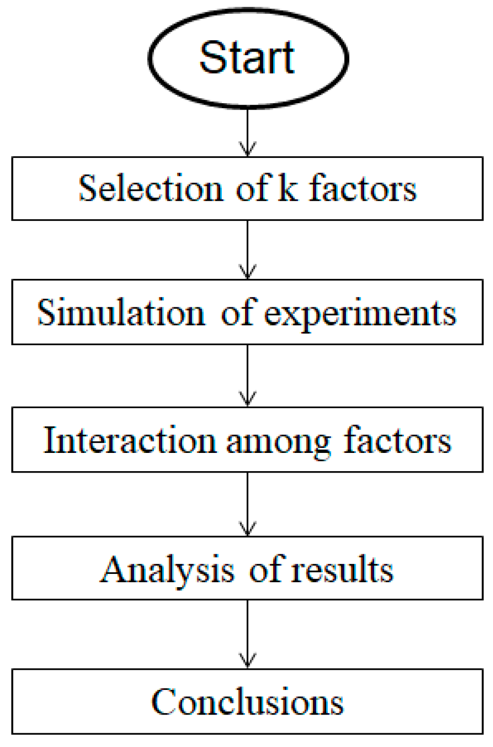
3. Factorial Methodology
3.1. Selection of k Factors
3.2. Simulations of Experiments
3.3. Interaction Among Factors
4. Results
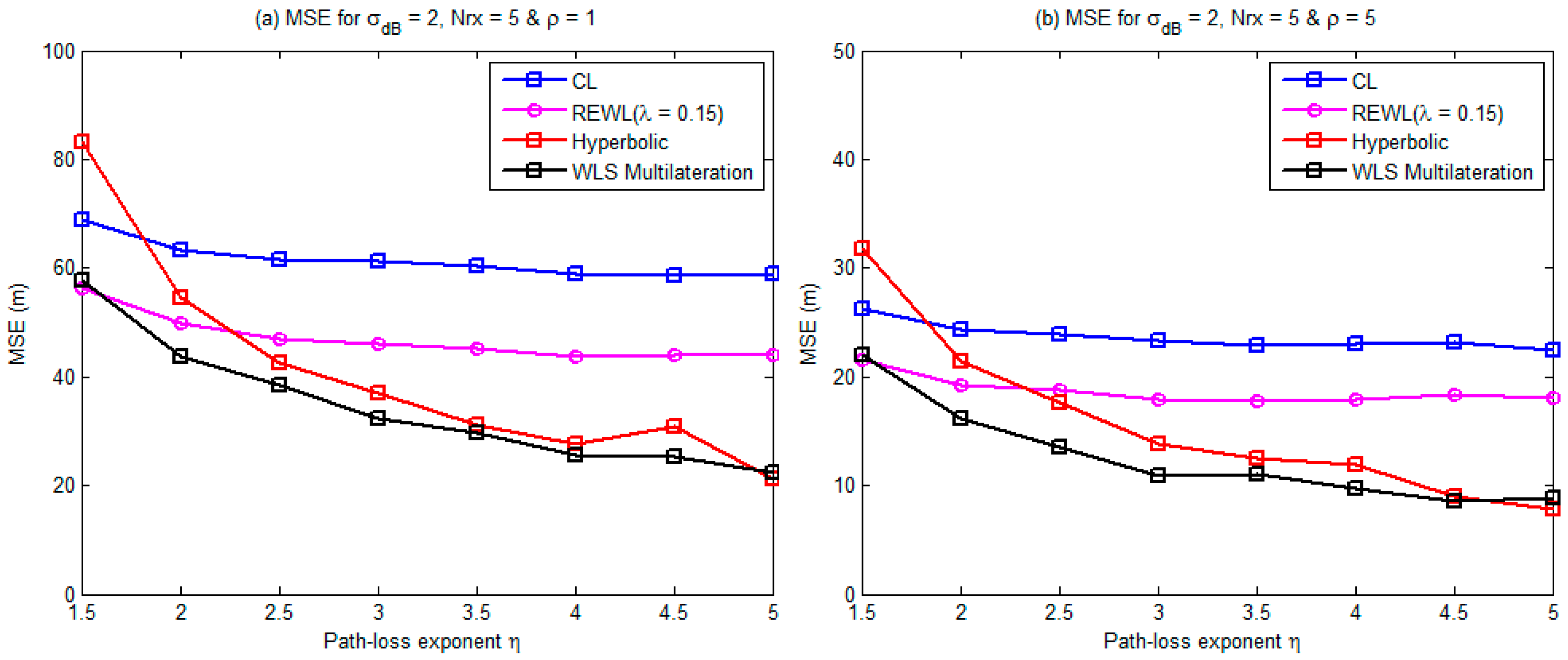
4.1. Path-Loss Exponent
4.2. Level Noise
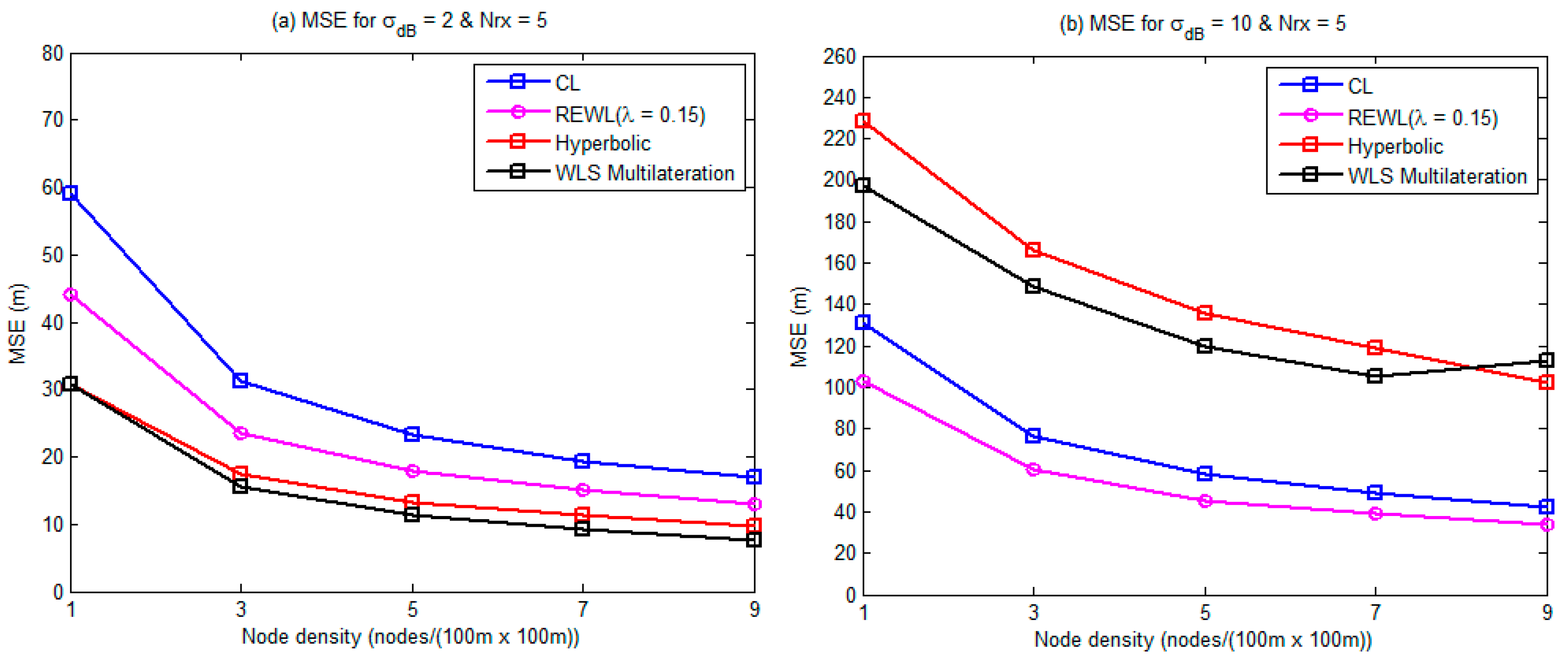
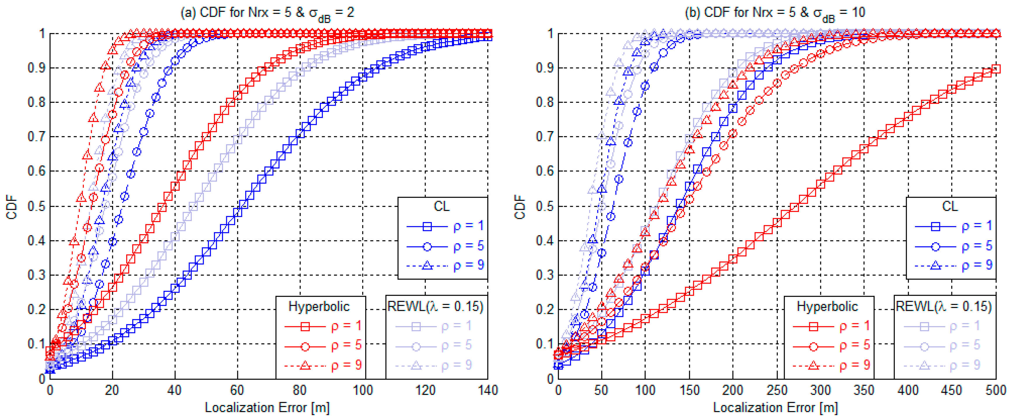
4.3. Node Density
4.4. Anchor Nodes
- –
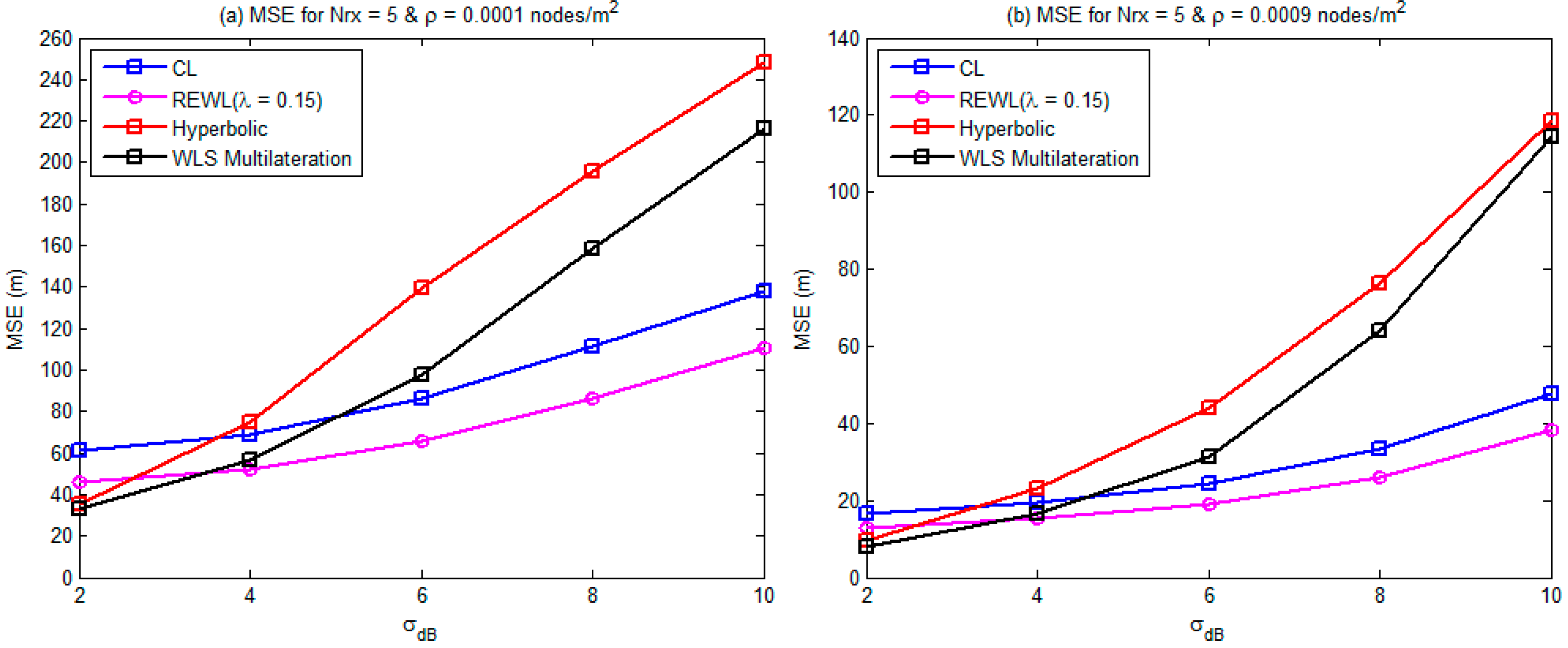
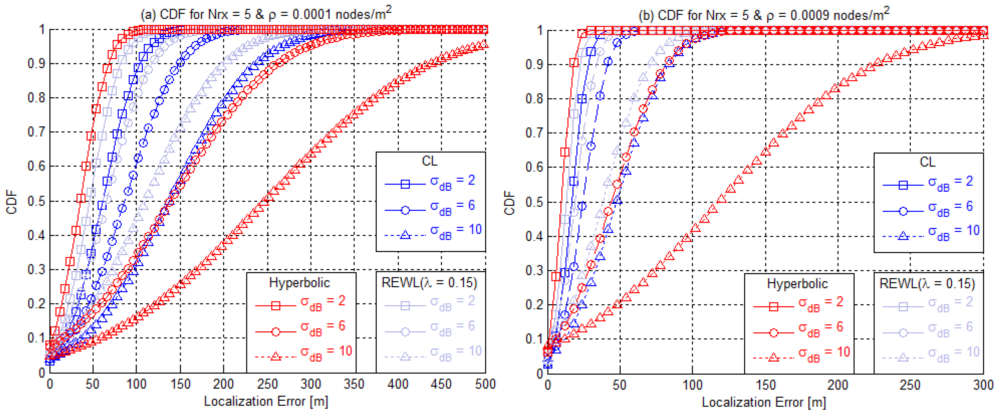
- The MSE and the CDF are affected to a great extent by the noise level , which shows a strong impact on range-based localization techniques.
- –
- The path-loss exponent has a greater impact on the MSE and the CDF of the range-based algorithms than on those of the range-free algorithms.
- –
- The combination of factors A and B shows greater impact on the MSE of the localization algorithms and very little on their CDF.
- –
- Node density has a greater impact on the MSE and the CDF of the range-free algorithms than on those of the range-based algorithms.
- –
- Node density is the factor that have the greatest impact on the localization algorithms’ CDF.
- –
- The path-loss exponent and the noise level are the factors that have the greatest impact on the localization algorithms’ MSE.
- –
- The number of RNs has zero impact on the range-based algorithms and shows very little impact on the CL algorithm’s MSE.
4.5. Impact of the Path-Loss Exponent.
4.6. Impact of Node Density
4.7. Impact of Noise Level
5. Conclusions
Author Contributions
Funding
Conflicts of Interest
References
- Dargie, W.; Poellabauer, C. Fundamentals of Wireless Sensor Networks: Theory and Practice; John Wiley & Sons: Hoboken, NJ, USA, 2010. [Google Scholar]
- Serna, M.A.; Casado, R.; Bermúdez, A.; Pereira, N.; Tennina, S. Distributed forest fire monitoring using wireless sensor networks. Int. J. Distrib. Sens. Netw. 2015, 11, 964564. [Google Scholar] [CrossRef]
- Rawat, P.; Singh, K.D.; Chaouchi, H.; Bonnin, J.M.-S. Wireless sensor networks: A survey on recent developments and potential synergies. J. Supercomput. 2014, 68, 1–48. [Google Scholar] [CrossRef]
- Carreño, P.; Gutierrez, F.; Ochoa, S.F.; Fortino, G. Using human-centric wireless sensor networks to support personal security. In Internet and Distributed Computing Systems; Pathan, M., Wei, G., Fortino, G., Eds.; Springer: Berlin/Heidelberg, Germany, 2013; Volume 8223, pp. 51–64. [Google Scholar]
- Ali, A.; Ming, Y.; Chakraborty, S.; Iram, S. A comprehensive survey on real-time applications of WSN. Future Internet 2017, 9, 77. [Google Scholar] [CrossRef]
- Chen, S.K.; Kao, T.; Chan, C.T.; Huang, C.N.; Chiang, C.Y.; Lai, C.Y.; Tung, T.-H.; Wang, P.C. A reliable transmission protocol for Zigbee-based wireless patient monitoring. IEEE Trans. Inf. Technol. Biomed. 2012, 16, 6–16. [Google Scholar] [CrossRef] [PubMed]
- Chang, Y.-J.; Chen, C.-H.; Lin, L.-F.; Han, R.-P.; Huang, W.-T.; Lee, G.-C. Wireless sensor networks for vital signs monitoring: application in a nursing home. Int. J. Distrib. Sens. Netw. 2012, 8, 1–12. [Google Scholar] [CrossRef]
- Egbogah, E.E.; Fapojuwo, A.O. A survey of system architecture requirements for health care-based wireless sensor networks. Sensors 2011, 11, 4875–4898. [Google Scholar] [CrossRef]
- Liu, N.; Cao, W.; Zhu, Y.; Zhang, J.; Pang, F.; Ni, J. The node deployment of intelligent sensor networks based on the spatial difference of farmland soil. Sensors 2015, 15, 28314–28339. [Google Scholar] [CrossRef]
- Valente, J.; Sanz, D.; Barrientos, A.; del Cerro, J.; Ribeiro, Á.; Rossi, C. An air-ground wireless sensor network for crop monitoring. Sensors 2011, 11, 6088–6108. [Google Scholar] [CrossRef]
- Saravanan, K.A.; Balaji, D. Cracker industry fire monitoring system over cluster based WSN. J. Eng. Appl. Sci. 2014, 9, 1–5. [Google Scholar]
- Wen, T.-H.; Jiang, J.-A.; Sun, C.-H.; Juang, J.-Y.; Lin, T.-S. Monitoring street-level spatial-temporal variations of carbon monoxide in urban settings using a wireless sensor network (WSN) framework. Int. J. Environ. Res. Public. Health 2013, 10, 6380–6396. [Google Scholar] [CrossRef]
- Yang, S.; Yang, X.; McCann, J.A.; Zhang, T.; Liu, G.; Liu, Z. Distributed networking in autonomic solar powered wireless sensor networks. IEEE J. Sel. Areas Commun. 2013, 31, 750–761. [Google Scholar] [CrossRef]
- Tan, R.; Xing, G.; Chen, J.; Song, W.-Z.; Huang, R. Fusion-based volcanic earthquake detection and timing in wireless sensor networks. ACM Trans. Sens. Netw. 2013, 9, 1–25. [Google Scholar] [CrossRef]
- Dyo, V.; Ellwood, S.A.; Macdonald, D.W.; Markham, A.; Trigoni, N.; Wohlers, R.; Mascolo, C.; Pásztor, B.; Scellato, S.; Yousef, K. WILDSENSING: Design and deployment of a sustainable sensor network for wildlife monitoring. ACM Trans. Sens. Netw. 2012, 8, 1–33. [Google Scholar] [CrossRef]
- Han, G.; Xu, H.; Duong, T.Q.; Jiang, J.; Hara, T. Localization algorithms of wireless sensor networks: A survey. Telecommun. Syst. 2013, 52, 2419–2436. [Google Scholar] [CrossRef]
- Chizhov, A.; Karakozov, A. Wireless sensor networks for indoor search and rescue operations. Int. J. Open Inf. Technol. 2017, 2, 1–4. [Google Scholar]
- Cheng, L.; Wu, C.; Zhang, Y.; Wu, H.; Li, M.; Maple, C. A survey of localization in wireless sensor network. Int. J. Distrib. Sens. Netw. 2012, 8, 1–12. [Google Scholar] [CrossRef]
- Vargas-Rosales, C.; Mass-Sánchez, J.; Ruiz-Ibarra, E.; Torres-Roman, D.; Espinoza-Ruiz, A. Performance evaluation of localization algorithms for WSNs. Int. J. Distrib. Sens. Netw. 2015, 11, 493930. [Google Scholar] [CrossRef]
- Iliev, N.; Paprotny, I. Review and comparison of spatial localization methods for low-power wireless sensor networks. IEEE Sens. J. 2015, 15, 5971–5987. [Google Scholar] [CrossRef]
- Chowdhury, T.J.S.; Elkin, C.; Devabhaktuni, V.; Rawat, D.B.; Oluoch, J. Advances on localization techniques for wireless sensor networks: A survey. Comput. Netw. 2016, 110, 284–305. [Google Scholar] [CrossRef]
- Laurendeau, C.; Barbeau, M. Centroid localization of uncooperative nodes in wireless networks using a relative span weighting method. EURASIP J. Wirel. Commun. Netw. 2010, 2010, 567040. [Google Scholar] [CrossRef]
- Zanca, G.; Zorzi, F.; Zanella, A.; Zorzi, M. Experimental Comparison of RSSI-Based Localization Algorithms for Indoor Wireless Sensor Networks. In Proceedings of the Workshop on Real-World Wireless Sensor Networks, Glasgow, UK, 1–4 April 2008. [Google Scholar]
- Jose Lopez, U.; Erica Ruiz, I.; Adolfo Espinoza, R.; Joaquin Cortez, G. Implementación y Evaluación de Algoritmos de Localización Libres de Distancia. In Proceedings of the Mexican International Conference on Computer Science 2016, Chihuahua, Mexico, 14–16 November 2016. [Google Scholar]
- Janssen, T.; Weyn, M.; Berkvens, R. Localization in low power wide area networks using wi-fi fingerprints. Appl. Sci. 2017, 7, 936. [Google Scholar] [CrossRef]
- Chang, S.; Li, Y.; He, Y.; Wang, H. Target localization in underwater acoustic sensor networks using RSS measurements. Appl. Sci. 2018, 8, 225. [Google Scholar] [CrossRef]
- Yoon, H.-S. Factorial design analysis for quality of video on MANET. Int. J. Comput. Electr. Autom. Contr. Inf. Eng. 2014, 8, 446–449. [Google Scholar]
- Aragão, M.V.; Frigieri, E.P.; Ynoguti, C.A.; Paiva, A.P. Factorial design analysis applied to the performance of SMS anti-spam filtering systems. Expert Syst. Appl. 2016, 64, 589–604. [Google Scholar] [CrossRef]
- Hakak, S.; Latif, S.A.; Anwar, F.; Alam, M.K.; Gilkar, G. Effect of 3 key factors on average end to end delay and jitter in MANET. J. ICT Res. Appl. 2014, 8, 113–125. [Google Scholar] [CrossRef]
- Cano, J.C.-G.; Manzoni, P.; Sanchez, M. Evaluating the Impact of Group Mobility on the Performance of Mobile Ad Hoc Networks. In Proceedings of the 2004 IEEE International Conference on Communications, Paris, France, 20–24 June 2004. [Google Scholar]
- Singh, S.P.; Sharma, S.C. Range free localization techniques in wireless sensor networks: A review. Procedia Comput. Sci. 2015, 57, 7–16. [Google Scholar] [CrossRef]
- Mass-Sanchez, J.; Ruiz-Ibarra, E.; Cortez-González, J.; Espinoza-Ruiz, A.; Castro, L.A. Weighted hyperbolic DV-hop positioning node localization algorithm in WSNs. Wirel. Pers. Commun. 2017, 96, 5011–5033. [Google Scholar] [CrossRef]
- Zhang, S.; Li, J.; He, B.; Chen, J. LSDV-hop: Least squares based DV-hop localization algorithm for wireless sensor networks. J. Commun. 2016, 11, 243–248. [Google Scholar] [CrossRef]
- Mass-Sanchez, J.; Ruiz-Ibarra, E.; Espinoza-Ruiz, A.; Rizo-Dominguez, L. A Comparative of Range Free Localization Algorithms and DV-Hop using the Particle Swarm Optimization Algorithm. In Proceedings of the 2017 IEEE 8th Annual Ubiquitous Computing, Electronics and Mobile Communication Conference, New York, NY, USA, 19–21 October 2017. [Google Scholar]
- Sun, S.; Yu, Q.; Xu, B. A node positioning algorithm in wireless sensor networks based on improved particle swarm optimization. Int. J. Future Gener. Commun. Net. 2016, 9, 179–190. [Google Scholar]
- Vargas-Rosales, C.; Munoz-Rodriguez, D.; Torres-Villegas, R.; Sanchez-Mendoza, E. Vertex projection and maximum likelihood position location in reconfigurable networks. Wirel. Pers. Commun. 2017, 96, 1245–1263. [Google Scholar] [CrossRef]
- Munoz, D.; Bouchereau, F.; Vargas, C.; Enriquez, R. Position Location Techniques and Applications; Elsevier/Academic Press: Cambridge, MA, USA, 2009. [Google Scholar]
- Frattini, F.; Esposito, C.; Russo, S. ROCRSSI++: An efficient localization algorithm for wireless sensor networks. Int. J. Adapt. Resilient Auton. Sys. 2011, 2, 51–70. [Google Scholar] [CrossRef]
- Will, H.; Hillebrandt, T.; Yuan, Y.; Yubin, Z.; Kyas, M. The Membership Degree Min-Max Localization Algorithm. In Proceedings of the 2012 Ubiquitous Positioning, Indoor Navigation, and Location Based Service (UPINLBS), Helsinki, Finland, 3–4 October 2012. [Google Scholar]
- Xie, S.; Hu, Y.; Wang, Y. An Improved E-Min-Max Localization Algorithm in Wireless Sensor Networks. In Proceedings of the 2014 IEEE International Conference on Consumer Electronics—China (ICCE-China 2014), Shenzhen, China, 9–13 April 2014. [Google Scholar]
- Bai, E.W.; Heifetz, A.; Raptis, P.; Dasgupta, S.; Mudumbai, R. Maximum likelihood localization of radioactive sources against a highly fluctuating background. IEEE Trans. Nucl. Sci. 2015, 62, 3274–3282. [Google Scholar] [CrossRef]
- Wagh, S.S.; More, A.; Kharote, P.R. Performance evaluation of IEEE 802.15. 4 protocol under coexistence of WiFi 802.11 b. Procedia Comput. Sci. 2015, 57, 745–751. [Google Scholar] [CrossRef]
- Jawad, H.; Nordin, R.; Gharghan, S.; Jawad, A.; Ismail, M. Energy-efficient wireless sensor networks for precision agriculture: A review. Sensors 2017, 17, 1781. [Google Scholar] [CrossRef] [PubMed]
- Xiong, W.; Hu, X.; Jiang, T. Measurement and characterization of link quality for IEEE 802.15. 4-compliant wireless sensor networks in vehicular communications. IEEE Trans. Ind. Inf. 2016, 12, 1702–1713. [Google Scholar] [CrossRef]
- Yang, S.-H. Wireless Sensor Networks: Principles Design and Applications; Springer: London, UK, 2014. [Google Scholar]
- Jiang, G.; Luo, M.; Bai, K.; Chen, S. A precise positioning method for a puncture robot based on a PSO-optimized BP neural network algorithm. Appl. Sci. 2017, 7, 969. [Google Scholar] [CrossRef]
- Fogue, M.; Garrido, P.; Martinez, F.J.; Cano, J.C.-G.; Calafate, C.T.; Manzoni, P. Analysis of the Most Representative Factors Affecting Warning Message Dissemination in VANETs under Real Roadmaps. In Proceedings of the 2011 IEEE 19th International Symposium on Modeling, Analysis & Simulation of Computer and Telecommunication Systems (MASCOTS), Singapore, 25–27 July 2011. [Google Scholar]
- Delgado, R.; Hernández, C.A.M.; Solís, R.R. Applying Design of Experiments to the Design of 60 GHz Antennas for Off-Body Communications. In Proceedings of the 2016 IEEE AP-S Symposium on Antennas and Propagation and USNC-URSI Radio Science Meeting, Fajardo, PR, USA, 25 June–2 July 2016. [Google Scholar]
- Rappaport, T.S. Wireless Communications: Principles and Practice, 2nd ed.; Prentice Hall: Upper Saddle River, NJ, USA, 2010. [Google Scholar]


| Localization Technique | Type | Description | Performance Metrics | Number of Hops | Simulation Environment |
|---|---|---|---|---|---|
| CL | range-free | This method calculates the position of the NOI as the centroid of the RNs. | MSE, CDF | One-Hop | Indoors Outdoors |
| WCL | range-free | Based on the CL algorithm considering a vector of weights, where these weights depend on the distance separating the NOI and the RNs. | MSE, CDF | One-Hop | Indoors Outdoors |
| RWL | range-free | Based on the WCL algorithm, where the vector of weights depends on a linear relation of the RSS between the NOI and the RNs. | MSE, CDF | One-Hop | Indoors Outdoors |
| REWL | range-free | Based on the WCL algorithm, where the vector of weights depends on an exponential relation of the RSS between the NOI and the RNs. | MSE, CDF | One-Hop | Indoors Outdoors |
| DV-Hop | range-free | This method calculates the average distance of a hop on the network, to estimate the distance separating the NOI from the RNs. | MSE, CDF | Multi-Hop | Outdoors |
| IDV-Hop | range-free | This technique takes the average of all the average distances per hop, to diminish the variance of the average distance per hop. | MSE, CDF | Multi-Hop | Outdoors |
| WDV-Hop | range-free | This technique considers the average distance per hop calculated by the IDV-Hop algorithm adding a compensation factor. | MSE, CDF | Multi-Hop | Outdoors |
| PSO | range-free | This localization algorithm calculates the position of the NOI as the overall optimum using an iterative process that minimizes the cost function. | MSE, CDF | Multi-Hop | Outdoors |
| Hyperbolic | range-based | This method converts the problem of non-linear localization into a linear problem using a least-squares estimator. | MSE, CDF | One-Hop Multi-Hop | Indoors Outdoors |
| Weighted Hyperbolic | range-based | This method converts the problem of non-linear localization into a linear problem using a weighted least-squares estimator. | MSE, CDF | One-Hop Multi-Hop | Indoors Outdoors |
| Circular | range-based | This method calculates the position of the NOI by iteratively using the descending gradient method until the cost function is minimized. | MSE, CDF | One-Hop Multi-Hop | Indoors Outdoors |
| WLS multilateration | range-based | This method converts the problem of non-linear localization into a linear problem using a weighted minimum-squares optimization algorithm. | MSE, CDF | One-Hop Multi-Hop | Indoors Outdoors |
| Vertex-Projection | range-based | Localization technique of low computational complexity based on a pyramid-shaped structure. | RMSE | One-Hop Multi-Hop | Outdoors |
| Vertex-Projection Correcting Factor | range-based | Considers a correction factor in the distance separating the NOI from the RNs, which diminishes the localization error. | RMSE | One-Hop Multi-Hop | Outdoors |
| Maximum-likelihood | range-based | This method uses the maximum-likelihood principle to estimate the distance separating the NOI from the RNs as a function of the number of hops. | RMSE | One-Hop Multi-Hop | Outdoors |
| LSDV-Hop | range-based | This method improves the precision of the NOI localization by extracting a minimum-squares transformation vector between the real and estimated position of the randomly selected RNs. | ALE | Multi-Hop | Outdoors |
| Symbol | Factor | Level −1 | Level 1 |
|---|---|---|---|
| A | Path-loss exponent | ||
| B | Level noise | 2 dB | 10 dB |
| C | Node density | ||
| D | Anchor nodes | 5 | 20 |
| Levels | MSE (m) | CDF (%) | |||||||||
|---|---|---|---|---|---|---|---|---|---|---|---|
| A | B | C | D | CL | REWL | Hyperbolic | WLS | CL | REWL | Hyperbolic | WLS |
| −1 | −1 | −1 | −1 | 69.76 | 57.39 | 78.1 | 57.91 | 5.829 | 8.2119 | 9.7503 | 11.31 |
| −1 | −1 | −1 | 1 | 127 | 87.85 | 104.45 | 73.04 | 5.663 | 7.5301 | 4.388 | 9.444 |
| −1 | −1 | 1 | −1 | 19.23 | 15.91 | 22.94 | 15.94 | 17.68 | 25.452 | 19.241 | 28.15 |
| −1 | −1 | 1 | 1 | 26.52 | 18.97 | 28.56 | 16.34 | 15.56 | 22.738 | 11.722 | 27.26 |
| −1 | 1 | −1 | −1 | 265.6 | 255.06 | 372.4 | 390.34 | 2.554 | 3.9807 | 1.8664 | 3.096 |
| −1 | 1 | −1 | 1 | 293.6 | 251.69 | 361.98 | 315.37 | 1.208 | 2.7236 | 0.2898 | 1.247 |
| −1 | 1 | 1 | −1 | 170.2 | 160.64 | 325.19 | 320.49 | 4.41 | 5.6936 | 4.2078 | 5.828 |
| −1 | 1 | 1 | 1 | 183.2 | 154.97 | 322.31 | 255.76 | 2.296 | 3.5721 | 0.2872 | 3.82 |
| 1 | −1 | −1 | −1 | 58.3 | 44.28 | 20.77 | 24.28 | 6.254 | 7.8482 | 23.726 | 25.25 |
| 1 | −1 | −1 | 1 | 108.2 | 43.61 | 16.63 | 10.19 | 6.29 | 9.2447 | 23.604 | 48.6 |
| 1 | −1 | 1 | −1 | 16.33 | 13.15 | 5.89 | 6.04 | 22.61 | 31.812 | 84.193 | 78.08 |
| 1 | −1 | 1 | 1 | 22.86 | 12.42 | 4.49 | 2.94 | 18.31 | 35.898 | 98.97 | 100 |
| 1 | 1 | −1 | −1 | 86.24 | 66.16 | 135.69 | 97.77 | 5.506 | 8.1518 | 8.5659 | 8.559 |
| 1 | 1 | −1 | 1 | 154.9 | 66.26 | 186.81 | 134.98 | 4.385 | 8.6823 | 1.8456 | 5.577 |
| 1 | 1 | 1 | −1 | 24.62 | 19.63 | 43.14 | 33.24 | 13.53 | 19.913 | 12.608 | 16.63 |
| 1 | 1 | 1 | 1 | 32.65 | 18.18 | 62.36 | 30.68 | 12.34 | 22.398 | 6.3494 | 14.2 |
| Factors | Variation Explained (%) | |||||||
|---|---|---|---|---|---|---|---|---|
| MSE (m) | CDF (%) | |||||||
| CL | REWL | Hyperbolic | WLS | CL | REWL | Hyperbolic | WLS | |
| A | 22.47 | 32.37 | 29.07 | 29.74 | 11.07 | 15.01 | 22.69 | 22.71 |
| B | 30.85 | 30.62 | 52.22 | 45.84 | 25.8 | 19.84 | 30.07 | 38.49 |
| C | 23.66 | 13.17 | 4.773 | 4.347 | 45.56 | 45.18 | 14.01 | 13.76 |
| D | 3.019 | 0.03 | 0.156 | 0.277 | 1.451 | 0.011 | 0.146 | 0.587 |
| AB | 17.68 | 21.48 | 13.18 | 18.25 | 2.622 | 1.821 | 13.86 | 11.14 |
| AC | 0.111 | 1.31 | 0.015 | 0.028 | 3.697 | 6.177 | 8.213 | 3.483 |
| AD | 0.04 | 0.046 | 0.048 | 0.489 | 0.006 | 0.854 | 0.211 | 1.147 |
| BC | 0.659 | 0.801 | 0.475 | 0.739 | 9.299 | 11.08 | 10.53 | 7.261 |
| BD | 0.000 | 0.113 | 0.021 | 0.26 | 0.006 | 0.022 | 0.215 | 1.425 |
| CD | 1.512 | 0.061 | 0.04 | 0.027 | 0.486 | 0.011 | 0.062 | 0.000 |
© 2018 by the authors. Licensee MDPI, Basel, Switzerland. This article is an open access article distributed under the terms and conditions of the Creative Commons Attribution (CC BY) license (http://creativecommons.org/licenses/by/4.0/).
Share and Cite
Mass-Sanchez, J.; Ruiz-Ibarra, E.; Gonzalez-Sanchez, A.; Espinoza-Ruiz, A.; Cortez-Gonzalez, J. Factorial Design Analysis for Localization Algorithms. Appl. Sci. 2018, 8, 2654. https://doi.org/10.3390/app8122654
Mass-Sanchez J, Ruiz-Ibarra E, Gonzalez-Sanchez A, Espinoza-Ruiz A, Cortez-Gonzalez J. Factorial Design Analysis for Localization Algorithms. Applied Sciences. 2018; 8(12):2654. https://doi.org/10.3390/app8122654
Chicago/Turabian StyleMass-Sanchez, Joaquin, Erica Ruiz-Ibarra, Ana Gonzalez-Sanchez, Adolfo Espinoza-Ruiz, and Joaquin Cortez-Gonzalez. 2018. "Factorial Design Analysis for Localization Algorithms" Applied Sciences 8, no. 12: 2654. https://doi.org/10.3390/app8122654
APA StyleMass-Sanchez, J., Ruiz-Ibarra, E., Gonzalez-Sanchez, A., Espinoza-Ruiz, A., & Cortez-Gonzalez, J. (2018). Factorial Design Analysis for Localization Algorithms. Applied Sciences, 8(12), 2654. https://doi.org/10.3390/app8122654