The Model Analysis of a Complex Tuning Fork Probe and Its Application in Bimodal Atomic Force Microscopy

Abstract

A new electromechanical coupling model was built to quantitatively analyze the tuning fork probes, especially the complex ones. A special feature of a novel, soft tuning fork probe, that the second eigenfrequency of the probe was insensitive to the effective force gradient, was found and used in a homemade bimodal atomic force microscopy to measure power dissipation quantitatively. By transforming the mechanical parameters to the electrical parameters, a monotonous and concise method without using phase to calculate the power dissipation was proposed.

1. Introduction

Quartz tuning forks are widely used in clocks, watches, and digital circuit frequency standards. By taking advantage of their extreme stability in frequency, their self-sensing and self-actuating capabilities, their high quality factor, and the ease with which the vibration signal may be obtained with fewer components than the conventional scanning probe microscopy (SPM) probes, etc., they can be used as force sensors in SPM [1,2,3,4,5]. The tuning fork probes are typically realized in two forms (Figure 1). The tip of the probe could be a carbon nanotube, an optical fiber, a conventional Atomic Force Microscopy (AFM) cantilever, or another type of stylus. With the development of some complex tuning fork probes [6,7], the quantitative use of the data (in terms of amplitude, phase, and frequency shifts) becomes challenging for these sophisticated probes. In this article, a kind of electromechanical coupling model with multistage coupling is proposed and used to describe a complex probe.

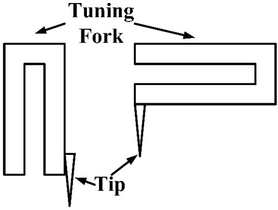
Figure 1. Normal tuning fork probes.

2. Modelling

The tuning fork probe can be seen as a mechanical oscillator in interaction with the surface by the tip. However, the output signal is current caused by the tuning fork’s piezoelectric effect. Tuning fork probes can be described by electromechanical coupling models [8,9,10].

A system’s differential equation of motion is

$$m\ddot{X}(t)+b\dot{X}(t)+kX(t)=F(t)$$

(1)

A circuit’s differential equation is

$$\frac{I(t)}{C}+L\ddot{I}(t)+R\dot{I}(t)=\dot{U}(t)$$

(2)

By comparing the Equations (1) and (2) after Laplace transformation as shown in Equation (3), the corresponding relationship of the electrical and mechanical parameters are shown in Table 1.

$$\begin{array}{l}m{s}^2+bs+k=\frac{F(s)}{X(s)}=\frac{F(s)s}{v(s)}\\ L{s}^2+Rs+\frac{1}{C}=\frac{U(s)s}{I(s)}\end{array}$$

(3)

Table 1. The corresponding relationship of the electrical and mechanical parameters.

Electrical	Mechanical
Inductance (L)	Mass (m)
Capacitance (C)	Reciprocal spring constant (1/k)
Resistance (R)	Damping (b)
Voltage (U)	Force (F)
Current (I)	Velocity (v)

The coupling can be regarded as an ideal transformer. According to the principle of the ideal transformer as shown in Figure 2a, the equivalent impedance Z′ in the left part is:

$$\begin{array}{l}\frac{U_1^2}{Z\prime }=\frac{U_2^2}{Z}\\ Z\prime =\frac{U_1^2}{U_2^2}Z=m^{2}Z\end{array}$$

(4)

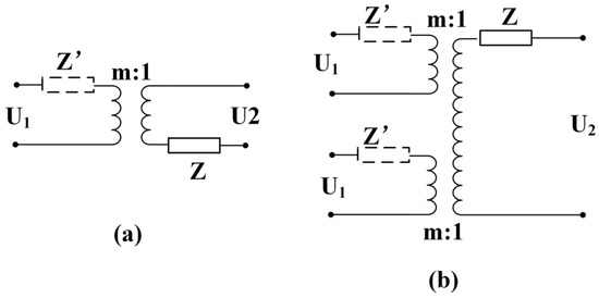
Figure 2. The ideal transformers.

And the relation between Z and Z′ in Figure 2b is

$$\begin{array}{l}\frac{2U_1^2}{Z\prime }=\frac{U_2^2}{Z}\\ \frac{U_1}{U_2}=\frac{m}{2}\\ Z\prime =\frac{2U_1^2}{U_2^2}Z=\frac{m^2}{2}Z\end{array}$$

(5)

2.1. The Model of Normal Tuning Fork Probes

At first, the multistage coupling model as shown in Figure 3 is utilized to specify normal tuning fork probes. The feature of the new model is two mechanical coupling stages are added to describe the cantilever (or the tip) and the sample respectively. The couplings are regarded as ideal transformers. All the mechanical parameters will be transformed to electrical parameters in an RLC circuit using the principle of ideal transformers.

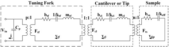
Figure 3. The electromechanical coupling model of normal probes.

This electromechanical coupling model consists of three parts: a typical electromechanical coupling part describing the tuning fork, a mechanical coupling part representing the connection between the cantilever (or tip) and the tuning fork, and another mechanical coupling part explaining the contact between the cantilever tip and the sample. In the model, the parameters, b, k, m, F, v, with different subscripts, denote damping, spring constant, mass, force, and the velocity of the tuning fork (subscript tf), and cantilever (subscript cl), respectively; C_p is the parasitic capacitance; i is the current; V_in is the excitation voltage; p is the electromechanical coupling factor; n, b_sa, and k_eff are the mechanical coupling factor, the damping, and effective force gradient between the tip and the sample. If the normal tuning fork’s tip is regarded as a rigid body, the spring constant (k_cl) of the tip is infinite and the damping (b_cl) is zero. The coupling factor between the tip and the tuning fork, and the factor between the tip and sample (factor n in Figure 3) are one because the tip is adhered to the tuning fork directly, v_tf = v_cl = v_tip. So the model can be transformed to:

With Equation (4), the model in Figure 4 can be transform to a simple RLC circuit as shown in Figure 5.

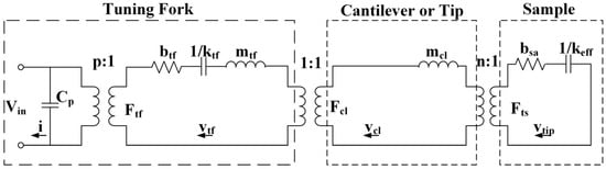
Figure 4. The model of rigid tip.

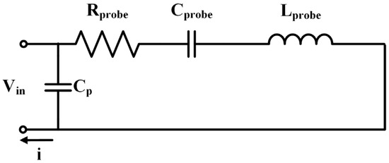
Figure 5. The equivalent RLC circuit of the tuning fork probe.

And the parameters in Figure 5 are

$$\begin{array}{l}{R}_{\mathrm{probe}}=p^2(b_{\mathrm{tf}}+b_{\mathrm{sa}})\\ L_{\mathrm{probe}}=p^2(m_{\mathrm{tf}}+m_{\mathrm{cl}})\\ C_{\mathrm{probe}}=\frac{1}{p^2(k_{\mathrm{tf}}+k_{\mathrm{eff}})}\end{array}$$

(6)

So the frequency shift after contact is

$$\begin{array}{l}\Delta f=f\prime -f_0=\frac{1}{2\mathsf{\pi }\sqrt{L_{\mathrm{probe}}C{\prime }_{\mathrm{probe}}}}-\frac{1}{2\mathsf{\pi }\sqrt{L_{\mathrm{probe}}{C}_{\mathrm{probe}}}}\\ =\frac{1}{2\mathsf{\pi }\sqrt{L_{\mathrm{probe}}C{\prime }_{\mathrm{probe}}{C}_{\mathrm{probe}}}}(\sqrt{C_{\mathrm{probe}}}-\sqrt{C{\prime }_{\mathrm{probe}}})\\ =\frac{f_0}{\sqrt{C{\prime }_{\mathrm{probe}}}}(\sqrt{C_{\mathrm{probe}}}-\sqrt{C{\prime }_{\mathrm{probe}}})\end{array}$$

(7)

$$\begin{array}{l}\frac{\Delta f}{f_0}=\sqrt{\frac{C_{\mathrm{probe}}}{C{\prime }_{\mathrm{probe}}}}-1\\ =\sqrt{\frac{k_{\mathrm{tf}}+k_{\mathrm{eff}}}{k_{\mathrm{tf}}}}-1\\ =\sqrt{1+\frac{k_{\mathrm{eff}}}{k_{\mathrm{tf}}}}-1\\ \Rightarrow {(\frac{\Delta f}{f_0})}^2+2(\frac{\Delta f}{f_0})=\frac{k_{\mathrm{eff}}}{k_{t\mathrm{f}}}\end{array}$$

(8)

For Δf << f₀,

$$k_{\mathrm{eff}}\approx 2\frac{\Delta f}{f_0}{k}_{\mathrm{tf}}$$

(9)

where k_tf is the spring constant of the tuning fork’s prong, Δf is the frequency shift, f₀ is the resonance frequency without contact. This equation is the same with the conclusion that regards the prong as a cantilever [11,12]. That means this model is correct to describe the normal tuning fork probes.

2.2. The Electromechanical Coupling Model of the Akiyama Probe

This kind of model also can be used to describe the tuning fork probes with complex structures. The Akiyama probe symmetrically couples a long, soft, U-shaped cantilever to a quartz tuning fork [7] (Figure 6). In this article, an electromechanical coupling model (Figure 7) with similar symmetrical structure is built to realize the quantitative analysis of the Akiyama probe.

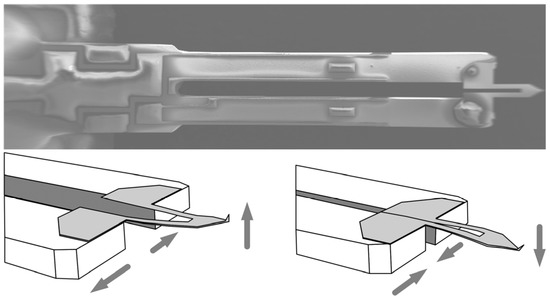
Figure 6. The appearance and motion (arrows in the figures) of the Akiyama probe.

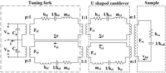
Figure 7. The electromechanical coupling model of an Akiyama probe.

This electromechanical coupling model consists of three parts: a typical electromechanical coupling part describing the tuning fork, a mechanical coupling part representing the connection between the cantilever and the tuning fork, and another mechanical coupling part explaining the contact between the cantilever tip and the sample. In the model, the parameters, b, k, m, F, v, with different subscripts, denote damping, spring constant, mass, force, and the velocity of the tuning fork (subscript tf), and cantilever (subscript cl), respectively; C_p is the parasitic capacitance; i is the current; V_in is the excitation voltage; p is the electromechanical coupling factor; n, b_sa, and k_eff are the mechanical coupling factor, the damping, and effective force gradient between the tip and the sample. The ends of the tuning fork prongs and the cantilever are stuck together, therefore, the coupling factor between the tuning fork and the cantilever is one.

2.2.1. The Transformation of the Model

With Equation (4), the cantilever part in Figure 7 can be transformed to the tuning fork part as shown in Figure 8.

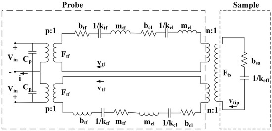
Figure 8. The transformation from cantilever to the tuning fork.

With Equation (5), the sample part in Figure 8 can be transformed to the probe as shown in Figure 9.

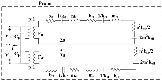
Figure 9. The transformation from sample to probe.

With Equation (4), the mechanical part in Figure 9 can be transformed to the electrical part as shown in Figure 10.

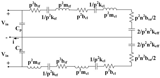
Figure 10. The transformation from mechanical parameters to electrical parameters.

As the two parts of the circuit are in parallel, the tuning fork prong’s electrical parameters are:

$$\begin{array}{l}{R}_{\mathrm{tf}}=\frac{p^2}{2}{b}_{\mathrm{tf}}\\ L_{\mathrm{tf}}=\frac{p^2}{2}{m}_{\mathrm{tf}}\\ C_{\mathrm{tf}}=\frac{2}{p^2{k}_{\mathrm{tf}}}\end{array}$$

(10)

where b_tf, m_tf, k_tf are damping, spring constant, mass of one of the tuning fork prongs. Factor p is the electromechanical coupling factor.

The cantilever’s electrical parameters are:

$$\begin{array}{l}{R}_{\mathrm{cl}}=\frac{p^2}{2}{b}_{\mathrm{cl}}\\ L_{\mathrm{cl}}=\frac{p^2}{2}{m}_{\mathrm{cl}}\\ C_{\mathrm{cl}}=\frac{2}{p^2{k}_{\mathrm{cl}}}\end{array}$$

(11)

The sample’s electrical parameters are:

$$\begin{array}{l}{R}_{\mathrm{sample}}=\frac{n^2{p}^2{b}_{\mathrm{sa}}}{4}\\ C_{\mathrm{sample}}=\frac{4}{n^2{p}^2{k}_{\mathrm{eff}}}\end{array}$$

(12)

The model can therefore be deemed equivalent to the circuit shown in Figure 11.

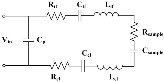
Figure 11. The equivalent electrical model of the Akiyama probe.

The electrical parameters of the equivalent circuit can be calculated as:

$$\begin{array}{l}{R}_{\mathrm{probe}}=R_{\mathrm{tf}}+R_{\mathrm{cl}}+R_{\mathrm{sample}}=\frac{p^2}{2}{b}_{\mathrm{tf}}+\frac{p^2}{2}{b}_{\mathrm{cl}}+\frac{p^2{n}^2{b}_{\mathrm{sa}}}{4}\\ L_{\mathrm{probe}}=L_{\mathrm{tf}}+L_{\mathrm{cl}}=\frac{p^2}{2}(m_{\mathrm{tf}}+m_{\mathrm{cl}})\\ C_{\mathrm{probe}}=\frac{1}{\frac{1}{C_{\mathrm{tf}}}+\frac{1}{C_{\mathrm{cl}}}+\frac{1}{C_{\mathrm{sample}}}}=\frac{1}{\frac{p^2}{2}{k}_{\mathrm{tf}}+\frac{p^2}{2}{k}_{\mathrm{cl}}+\frac{n^2{p}^2}{4}{k}_{\mathrm{eff}}}\end{array}$$

(13)

The final RLC circuit is shown as Figure 5.

So when k_eff = 0, the resonant frequency of the probe without contact is:

$$f_0=\frac{1}{2\mathsf{\pi }\sqrt{L_{\mathrm{probe}}{C}_{\mathrm{probe}}}}=\frac{1}{2\mathsf{\pi }\sqrt{\frac{\frac{p^2}{2}(m_{\mathrm{tf}}+m_{\mathrm{cl}})}{\frac{p^2}{2}(k_{\mathrm{tf}}+k_{\mathrm{cl}})}}}=\frac{1}{2\mathsf{\pi }}\sqrt{\frac{k_{\mathrm{tf}}+k_{\mathrm{cl}}}{m_{\mathrm{tf}}+m_{\mathrm{cl}}}}=\frac{1}{2\mathsf{\pi }}\sqrt{\frac{k_{\mathrm{probe}}}{m_{\mathrm{probe}}}}$$

(14)

The resonant frequency after touching the sample is:

$$f\prime =\frac{1}{2\mathsf{\pi }}\sqrt{\frac{k_{\mathrm{probe}}+\frac{n^2}{2}{k}_{\mathrm{eff}}}{m_{\mathrm{probe}}}}$$

(15)

2.2.2. The Verification of the Model

For proving the validity of this electromechanical coupling model of an Akiyama probe, finite element analysis (FEA) software (ANSYS, 14.0, ANSYS Inc., Canonsburg, PA, USA, 2011), is used to simulate the contact between the tip and the sample [13]. The parameters of the Akiyama probe used to build the model are shown in Table 2.

Table 2. The parameters of ANSYS simulation.

Parameters	Tuning Fork	Cantilever
Length/μm	2400	175
Thickness/μm	220	31.9
Width/μm	103.7	3.7
Density/kg·m−3	2290	2300
Young modulus/GPa	78.7	180

The contact between the tip and the sample is simulated by a spring as shown in Figure 12 and the spring constant represents the effective force gradient between the tip and the sample (k_eff). Where k_eff is

$$k_{\mathrm{eff}}=⟨\nabla F_{\mathrm{ts}}⟩$$

(16)

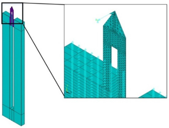
Figure 12. The ANSYS model of an Akiyama probe.

The F_ts is the force between the tip and sample, it can be described as follows in DMT model:

$$F_{\mathrm{ts}}=\{\begin{array}{l}\frac{F_0}{{(1-\frac{a_0-z}{a_0})}^2},z\ge a_0\\ -\frac{4}{3}{E}^{*}\sqrt{R}{(a_0-z)}^{\frac{3}{2}}+F_0,z<a_0\end{array}$$

(17)

where F₀ is the adhesive force, z is the distance between the tip and sample, a₀ is the radius of the atom, R is the radius of the tip, and E* is

$$\frac{1}{E^{*}}=\frac{1-v_{\mathrm{s}}^2}{E_{\mathrm{s}}}+\frac{1-v_{\mathrm{t}}^2}{E_{\mathrm{t}}}$$

(18)

where E_s, E_t are the Young’s modulus of the sample and the tip, v_s, v_t are the poisson ratio of the sample and the tip.

In the simulation, a constant k_eff is used, which means the maximal F_ts is

$$F_{\max }=k_{\mathrm{eff}}A$$

(19)

where A is the amplitude of the cantilever.

The results of the non-contact simulation are shown in Table 3.

Table 3. The results of ANSYS simulation.

Resonance Frequency/Hz	Tuning Fork Amplitude Dtf/m	Charge q/C	Cantilever Amplitude Dcl/m
52,888	1.26 × 10−7	3.73 × 10−13	3.36 × 10−6

Coupling factors, p and n, can therefore be calculated as:

$$\begin{array}{l}p=\frac{2v_{\mathrm{tf}}}{i}=\frac{2\mathsf{\omega }{D}_{\mathrm{tf}}}{\mathsf{\omega }q}=\frac{2D_{\mathrm{tf}}}{q}=6.76\times {10}^5\mathrm{m}/\mathrm{C}\\ n=\frac{v_{\mathrm{tip}}}{v_{\mathrm{tf}}}=\frac{\mathsf{\omega }{D}_{\mathrm{tip}}}{\mathsf{\omega }{D}_{\mathrm{tf}}}=\frac{D_{\mathrm{tip}}}{D_{\mathrm{tf}}}=26.67\end{array}$$

(20)

The tuning fork prong is always represented by rectangular cantilever, the spring constant, and effective mass can be calculated as:

$$\begin{array}{l}k=\frac{1}{4}Ew{(\frac{t}{l})}^3=1571.55\mathrm{N}/\mathrm{m}\\ m=0.24\mathsf{\rho }wtl=3.01\times {10}^{-8}\mathrm{kg}\end{array}$$

(21)

The resonant frequency with contact can be expressed as:

$$f\prime =\frac{1}{2\mathsf{\pi }}\sqrt{f_0^2+\frac{n^2{k}_{\mathrm{eff}}}{2m_{\mathrm{probe}}}}$$

(22)

The effective mass of the U-shaped cantilever is difficult to calculate. If this mass is 0.001m_probe for example, the error in the resonant frequency after ignoring this mass will be:

$$f_1^2-f_2^2=\frac{1}{4{\mathsf{\pi }}^2}(\frac{n^2{k}_{\mathrm{eff}}}{m_{\mathrm{probe}}}-\frac{n^2{k}_{\mathrm{eff}}}{1.001m_{\mathrm{probe}}})<0.001\times \frac{1}{4{\mathsf{\pi }}^2}\frac{n^2{k}_{\mathrm{eff}}}{m_{\mathrm{probe}}}$$

(23)

$$f_1-f_2=\frac{f_1^2-f_2^2}{f_1+f_2}<0.001\times \frac{1}{4{\mathsf{\pi }}^2}\frac{n^2{k}_{\mathrm{eff}}}{m_{\mathrm{probe}}}\frac{1}{2f_0}$$

(24)

When the value of k_eff is small enough, 0.01 N/m for example, the error is less than 1 Hz, so the effective mass of the U-shaped cantilever can be ignored during the calculation of the resonant frequency and the spring constant of the probe is given by:

$$k_{\mathrm{probe}}=k_{\mathrm{tf}}+k_{\mathrm{cl}}=4{\mathsf{\pi }}^2{f}_0^2{m}_{t\mathrm{f}}=3323.84\mathrm{N}/\mathrm{m}$$

(25)

Using the parameters calculated above, the resonant frequencies for different values of k_eff can be obtained from Equation (15). Compared with the results of ANSYS simulation as shown in Table 4, the revised electromechanical coupling model can describe the Akiyama probe correctly when the value of k_eff is small. For an average force, between the tip and sample, in tapping mode of typically less than 1 nN, k_eff is less than 0.001 N/m in this simulation: the electromechanical coupling model of the Akiyama probe is accurate as evinced by simulation data.

Table 4. The results of ANSYS simulation with different values of k_eff.

keff (N/m)	ANSYS/Hz	n	Model/Hz	Deviation/Hz
0	52,888	13.38	52,888	0
0.001	52,890	12.92	52,891	1
0.005	52,896	11.18	52,898	2
0.01	52,901	9.49	52,902	1
0.02	52,909	7.15	52,904	−5

2.2.3. The Measurement of the Coupling Factors

The calculation of the real probe’s electromechanical coupling factor uses the vibration amplitude of the tuning fork and the output current of the probe. The factor n is calculated by measuring the amplitude of the tuning fork and the cantilever. All the vibration amplitudes are measured by laser Doppler vibrometer (OFV-3001, Polytec, Waldbronn, Germany). The measured points of the tuning fork and the cantilever are shown in Figure 13.

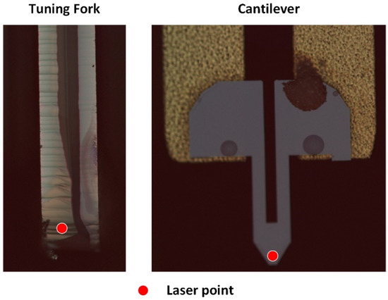
Figure 13. The measurement of factors using laser Doppler vibrometer.

2.3. Feature of the Second Eigenmode

In Equation (15), the coupling factor n determines the influence of k_eff on the frequency modulation (FM) mode sensitivity. If n > 1, the influence is magnified, otherwise, it is reduced. In the first eigenmode as simulated above, n = 26.67, implying that the resonant frequency is quite sensitive to the value of k_eff; but in the second eigenmode (Table 5), n < 1, and the sensitivity thereto is very low, and the simulation results show that the resonance frequency will not change as k_eff increases.

Table 5. The second eigenmode results: ANSYS simulation with different values of k_eff.

keff (N/m)	Resonance Frequency/Hz	Charge/C	Tuning Fork Amplitude/m	Cantilever Amplitude/m
0	206,153	2.07 × 10−13	2.93 × 10−8	1.03 × 10−9
0.0001	206,153	2.07 × 10−13	2.93 × 10−8	1.03 × 10−9
0.001	206,153	2.07 × 10−13	2.93 × 10−8	1.03 × 10−9
0.01	206,153	2.07 × 10−13	2.93 × 10−8	1.03 × 10−9
0.1	206,153	2.07 × 10−13	2.93 × 10−8	1.03 × 10−9

The second eigenfrequency of the Akiyama probe is not sensitive to k_eff, which means that the eigenfrequency is stable when the tip makes contact with the sample. This is a drawback when studying the relationship between the second eigenfrequency and the contact stiffness. However, the constant resonant frequency means that the amplitude is related to energy dissipation directly.

The amplitude change in amplitude modulation (AM) mode can be divided into two parts as shown in Figure 14. If the resonant frequency is constant, ΔA_k = 0, ΔA = ΔA_b, the amplitude change is caused only by the energy dissipation.

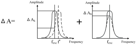
Figure 14. The division of the amplitude change in AM mode.

2.4. The Calculation of the Power Dissipation

With the electromechanical coupling model of an Akiyama probe, the power dissipation caused by damping effects in the sample under test is:

$$P_{\mathrm{dis}}=\frac{1}{2}{b}_{\mathrm{sa}}{D}_{tip}^2{\mathsf{\omega }}^2=\frac{1}{2}{b}_{\mathrm{sa}}{v}_{\mathrm{tip}}^2=\frac{1}{2}{b}_{\mathrm{sa}}{(\frac{1}{2}pni)}^2=\frac{1}{2}(\frac{1}{4}{p}^2{n}^2{b}_{\mathrm{sa}})i^2=\frac{1}{2}{i}^2{R}_{\mathrm{sample}}$$

(26)

Given the definition in Equation (13), with parasitic capacitance (C_p) compensation, the impedance of the circuit in Figure 5 is:

$$Z(\mathsf{\omega })=R_{\mathrm{probe}}+j\mathsf{\omega }{L}_{\mathrm{probe}}+\frac{1}{j\mathsf{\omega }{C}_{\mathrm{probe}}}=\frac{j\mathsf{\omega }{R}_{\mathrm{probe}}{C}_{\mathrm{probe}}+[1-{(\frac{\mathsf{\omega }}{{\mathsf{\omega }}_0})}^2]}{j\mathsf{\omega }{C}_{\mathrm{probe}}}$$

(27)

When the circuit is resonance oscillating, ω = ω₀, the non-contact impedance is:

$$Z({\mathsf{\omega }}_0)=R_{\mathrm{probe}}=\frac{p^2}{2}(b_{\mathrm{tf}}+b_{\mathrm{cl}})$$

(28)

The contact impedance is:

$$Z\prime ({\mathsf{\omega }}_0\prime )=R_{\mathrm{probe}}+R_{\mathrm{sample}}=\frac{p^2}{2}(b_{\mathrm{tf}}+b_{\mathrm{cl}}+\frac{1}{2}{n}^2{b}_{\mathrm{sa}})$$

(29)

As mentioned above, the resonant frequency is not changed, so ω₀ = ω₀′, and the change in current is given by:

$$\Delta I=\frac{U}{Z({\mathsf{\omega }}_0)}-\frac{U}{Z\prime ({\mathsf{\omega }}_0\prime )}=U\frac{R_{\mathrm{sample}}}{R_{\mathrm{probe}}+(R_{\mathrm{probe}}+R_{\mathrm{sample}})}=I\prime \frac{R_{\mathrm{sample}}}{R_{\mathrm{probe}}}$$

(30)

where U is the input voltage, I′ is the current after contact. With Equations (26) and (30), the power dissipation is given by:

$$P_{\mathrm{diss}}=\frac{1}{2}I{\prime }^2{R}_{\mathrm{sample}}=\frac{1}{2}I{\prime }^2\frac{\Delta I}{I\prime }{R}_{\mathrm{probe}}=\frac{1}{2}I\prime \Delta I{R}_{\mathrm{probe}}=\frac{1}{2}\frac{UI\prime (I-I\prime )}{I}$$

(31)

where I is the current without contact.

The classical equation using phase to calculate the power dissipation is [14]:

$$P_{\mathrm{diss}}=\frac{1}{2}\frac{k\mathsf{\omega }}{Q}(A_{0}A\sin \mathsf{\phi }-A^2\frac{\mathsf{\omega }}{{\mathsf{\omega }}_0})$$

(32)

where k is the spring constant of the probe, Q is the quality factor, A₀ and A are the amplitude with or without contact, ω is the exciting frequency, ω₀ is the resonance frequency, ϕ is the phase. When ω = ω₀, the equation become:

$$P_{\mathrm{diss}}=\frac{1}{2}\frac{k{\mathsf{\omega }}_0}{Q}(A_{0}A\sin \mathsf{\phi }-A^2)$$

(33)

For

$$\begin{array}{l}Q=\frac{\sqrt{km}}{b}\\ k={\mathsf{\omega }}_0^{2}m\end{array}$$

(34)

Then,

$$\begin{array}{l}{P}_{\mathrm{diss}}=\frac{1}{2}b{\mathsf{\omega }}_0^2(A_{0}A\sin \mathsf{\phi }-A^2)\\ =\frac{1}{2}b[(A_0{\mathsf{\omega }}_0)(A{\mathsf{\omega }}_0)\sin \mathsf{\phi }-{(A{\mathsf{\omega }}_0)}^2]\\ =\frac{1}{2}b(v_{0}v\sin \mathsf{\phi }-v^2)\end{array}$$

(35)

where k is the spring constant of the probe, Q is the quality factor, A₀ and A are the amplitude with or without contact, ω is the exciting frequency, ω₀ is the resonance frequency, ϕ is the phase, b is the damping of the probe, v₀ and v are the velocity with or without contact. When the probe is kept at resonance, ϕ = 90°, and with the corresponding relationship in Table 1, the two methods are equivalent.

$$P_{\mathrm{diss}}=\frac{1}{2}b(v_{0}v-v^2)\iff \frac{1}{2}{R}_{\mathrm{probe}}(II\prime -I{\prime }^2)$$

(36)

By electromechanical coupling, Equation (31) is equivalent to Equation (32) when the excitation frequency is kept at the resonance frequency during the scanning as the feature of the Akiyama probe is working in the second eigenmode. So Equation (31) is correct.

3. Measuring System

The bimodal AFM measuring system based on the Akiyama probe shown in Figure 15 is built to utilize this feature to measure the power dissipation. Two lock-in amplifications (LIA) excite the probe and demodulate the output signal. The first eigenmode signal amplitude is sent to the feedback system to control the PZT (piezoelectric ceramic transducer) to keep the distance between the tip and the sample constant as normal tapping mode, the position of the PZT describes the morphology of the sample. The second eigenmode signal amplitude is recorded, as mentioned above, this is related to the power dissipation therein.

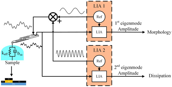
Figure 15. The Schematic of bimodal AFM based on an Akiyama probe.

The setpoint of the first eigenmode signal is 0.6 A₀₁, the amplitude ratio of the two signals is A₀₁/A₀₂ = 0.723 V/0.503 V ≈ 1.437, where A₀₁ and A₀₂ are the amplitude of the first and the second eigenmode signals without contact. Parameters of the probe: the eigenfrequencies are f₀₁ = 46.162 kHz, f₀₂ = 202.646 kHz, cantilever spring constant k ≈ 5 N/m, quality factors: Q₁ = 1154, Q₂ = 6776. The scanning speed is 250 nm/s. There are 220 measured points along the length of 8760 nm.

4. Results and Discussion

The sample consists of Au wire on a SiO₂ substrate, the height of the Au wire is about 150 nm. The sample is coated with a 20 nm thick Cr layer as shown in Figure 14 to obtain the similar surface Young’s modulus (SiO₂ substrate: 113.665 ± 4.031 Gpa, Au substrate: 119.382 ± 12.734 Gpa, measured by a nano indenter, Agilent Technologies Inc., Santa Clara, CA, USA). Figure 16 shows the results of a line on the sample and all the lines’ results are averaged and listed in Table 6.

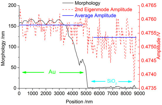
Figure 16. The profile of the sample.

Table 6. The results of tests on the Micro-Electro-Mechanical System (MEMS) sample at intervals of 1 μm.

Substrate	Au/nW	SiO2	Deviation
Line 1	0.599	0.609	10
Line 2	0.594	0.599	5
Line 3	0.591	0.596	5
Line 4	0.589	0.598	9
Line 5	0.585	0.597	12
Average	0.591	0.600	8
Standard Deviation	5	10	3

For the uniform surfaces of the two parts, the difference of power dissipation is only caused by the different substrates. The deviation between the two parts are stable in Table 6, the power dissipation of the Au substrate is less than the SiO₂ substrate. The repeatable results mean this method is credible.

5. Conclusions

In conclusion, with the help of an electromechanical coupling model, a special feature of a tuning fork probe with complex structure is found and utilized to measure power dissipation. According to the model, the insensitive second eigenfrequency and the relation between the output current and the power dissipation are illustrated. In Equation (31), there are no mechanical parameters of the probe and the electrical parameters are easy to measure. Different to the complex and non-monotonous method using phase to calculate the power dissipation, the Equation (31) is not necessary to calibrate the probe’s spring constant which is still hard to measure accurately. With the monotonous relation between the current and the sample’s damping, the contrast of the image is stable.

References

- De Oteyza, D.G.; Gorman, P.; Chen, Y.C.; Wickenburg, S.; Riss, A.; Mowbray, D.J.; Etkin, G.; Pedramrazi, Z.; Tsai, H.-Z.; Rubio, A.; et al. Direct imaging of covalent bond structure in single-molecule chemical reactions. Science 2013, 340, 1434–1437. [Google Scholar] [CrossRef] [PubMed]
- Bontempi, A.; Teyssieux, D.; Friedt, J.M.; Thiery, L.; Hermelin, D.; Vairac, P. Photo-thermal quartz tuning fork excitation for dynamic mode atomic force microscope. Appl. Phys. Lett. 2014, 105, 154104. [Google Scholar] [CrossRef]
- Ichii, T.; Fujimura, M.; Negami, M.; Murase, K.; Sugimura, H. Frequency modulation atomic force microscopy in ionic liquid using quartz tuning fork sensors. Jpn. J. Appl. Phys. 2012. [Google Scholar] [CrossRef]
- González, L.; Oria, R.; Botaya, L.; Puig-Vidal, M.; Otero, J. Determination of the static spring constant of electrically-driven quartz tuning forks with two freely oscillating prongs. Nanotechnology 2015, 26, 055501. [Google Scholar] [CrossRef] [PubMed]
- Oiko, V.T.A.; Martins, B.V.C.; Silva, P.C.; Rodrigues, V.; Ugarte, D. Development of a quartz tuning-fork-based force sensor for measurements in the tens of nanoNewton force range during nanomanipulation experiments. Rev. Sci. Instrum. 2014, 85, 035003. [Google Scholar] [CrossRef] [PubMed]
- Nishi, R.; Houda, I.; Kitano, K.; Sugawara, Y.; Morita, S. A noncontact atomic force microscope in air using a quartz resonator and the FM detection method. Appl. Phys. A 2001, 72, S93–S95. [Google Scholar] [CrossRef]
- Akiyama, T.; de Rooij, N.F.; Staufer, U.; Detterbeck, M.; Braendlin, D.; Waldmeier, S.; Scheidiger, M. Implementation and characterization of a quartz tuning fork based probe consisted of discrete resonators for dynamic mode atomic force microscopy. Rev. Sci. Instrum. 2010, 81, 063706. [Google Scholar] [CrossRef] [PubMed]
- Babic, B.; Hsu, M.T.L.; Gray, M.B.; Lu, M.; Herrmann, J. Mechanical and electrical characterization of quartz tuning fork force sensors. Sens. Actuators A 2015, 223, 167–173. [Google Scholar] [CrossRef]
- Patimisco, P.; Sampaolo, A.; Dong, L.; Giglio, M.; Scamarcio, G.; Tittel, F.K.; Spagnolo, V. Analysis of the electro-elastic properties of custom quartz tuning forks for optoacoustic gas sensing. Sens. Actuators B 2016, 227, 539–546. [Google Scholar] [CrossRef]
- Qin, Y.; Reifenberger, R. Calibrating a tuning fork for use as a scanning probe microscope force sensor. Rev. Sci. Instrum. 2007, 78, 063704. [Google Scholar] [CrossRef] [PubMed]
- Acosta, J.C.; Hwang, G.; Polesel-Maris, J.; Régnier, S. A tuning fork based wide range mechanical characterization tool with nanorobotic manipulators inside a scanning electron microscope. Rev. Sci. Instrum. 2011, 82, 035116. [Google Scholar] [CrossRef] [PubMed]
- Van, V.D.; Lange, M.; Schmuck, M.; Schmidt, N.; Möller, R. Spring constant of a tuning-fork sensor for dynamic force microscopy. Beilstein J. Nanotechnol. 2012, 3, 809–816. [Google Scholar]
- Zhao, J. Study on Development of Self-Sensing AFM Head and Hybrid Measurement System. Ph.D. Thesis, Tianjin University, Tianjin, China, 2011. [Google Scholar]
- Balantekin, M.; Atalar, A. Power dissipation analysis in tapping-mode atomic force microscopy. Phys. Rev. B 2003, 67, 193404. [Google Scholar] [CrossRef]
© 2017 by the authors. Licensee MDPI, Basel, Switzerland. This article is an open access article distributed under the terms and conditions of the Creative Commons Attribution (CC BY) license ( http://creativecommons.org/licenses/by/4.0/).