A GTA Welding Cooling Rate Analysis on Stainless Steel and Aluminum Using Inverse Problems

Abstract

This work presents an analysis of the thermal influence of the heat transfer by convection and radiation during GTA (gas tungsten arc) welding process. The authors’ in-house C++ previously-developed code was modified to calculate the amount of heat transfer by convection and radiation. In this software, an iterative Broydon-Fletcher-Goldfarb-Shanno (BFGS) inverse method was applied to estimate the amount of heat delivered to the plate when the appropriate sensitivity criteria were defined. The methodology was validated by accomplishing lab-controlled experiments on stainless steel AISI 304L and aluminum 6065 T5 plates. Due to some experimental singularities, the forced thermal convection induced by the electromagnetic field and thermal-capillary force were disregarded. Significant examples of these singularities are the relatively small weld bead when compared to the sample size and the reduced time of the welding process. In order to evaluate the local Nusselt number, empirical correlations for flat plates were used. The thermal emission was a dominant cooling effect on the aluminum cooling. However, it did not present the same behavior as the stainless steel samples. The study found that the heat losses by convection and radiation of the weld pool do not affect the cooling process significantly.

1. Introduction

The gas tungsten arc (GTA) welding process is largely used in industrial applications nowadays. Due to its great welding quality and low equipment cost, this process is extensively applied to stainless steel, titanium alloy, and non-ferrous metals welds [1]. In the GTA welding process, a tungsten electrode is protected by a flow of inert gas; argon is usually employed, as well as helium, nitrogen, hydrogen, or mixtures. The knowledge of the heat flux, temperature gradients, and cooling process are thoroughly necessary for welding process studies. The thermal analysis is fundamentally based on models of heat transfer theory, which include the following phenomena: specific heat, latent heat, two-phase regions, moving interfaces, conservation of energy, fluid mechanics, conductivity, contact resistance, radiation emissivity, and convection [2].

The weld quality depends on several parameters that control the temperature of the workpiece. For instance, the electric current and the torch speed are important factors in the GTA welding process [3,4]. The cooling rate is an important factor that affects all welding process quality. Heat loss, which occurs due to diffusion, free convection, and radiation, occur spontaneously; therefore, it is difficult to control the cooling rate during the welding process. There are several ways to control the heat loss in a welding process; one of them is to control the heat diffusion on the workpiece by preheating of the sample [5]. Another one is to perform the process in a vacuum room, which will obliterate the free convection [6]. However, the thermal emission of radiation cannot be estimated. As a matter of fact, any matter at a temperature higher than absolute zero will emit thermal radiation, which limits the control.

Several authors have been studying numerical models for the welding process. These models satisfactorily predict the temperature at the peak point [7,8]. However, they fail to analyze the cooling rate because they use simple approaches for the radiation and heat transfer coefficient by convection. For instance, Gonçalves et al. [7] used a three-dimensional model based on the diffusion equation and the enthalpy method to model a TIG welding process. The authors’ model used an empirical correction to estimate the heat transfer coefficient in the sample. However, this model did not consider the thermal emission by radiation. Thus, as expected, the model failed to predict the temperature after the TIG welding torch was turned off. The same pattern is seen in Aissani et al. [8]. In their work, the authors model a TIG welding process for the same stainless steel of Gonçalves et al. [7]. They used a linearization of the radiation equation of the Stefan-Boltzmann law and a constant heat transfer coefficient for the convection analysis. Although the authors’ model covers radiation and convection, the use of a linear approach in a welding model is not recommended due to the high thermal gradient characteristic of the process. The author’s model predicts the heating part of the problem well; on the other hand, it fails to analyze the cooling rate part.

In Magalhães et al. [9] previous work a numerical software, based on an inverse problem and enthalpy method, was developed in order to predict the thermal field in a GTA aluminum welding. The thermal field in any region of the plate or anytime was determined through the numerical solution of the three-dimensional heat diffusion equation. The inverse technique of BFGS was used to estimate the heat applied in the process. The finite difference method and the implicit Euler method for time discretization were used to solve the heat diffusion equation.

Some improvements are made in relation to the previous work. In this work, a detailed analysis of the cooling rate is presented. Furthermore, the heat losses are presented separately under two headings: convection and radiation. In the same way, a comparison between the thermal fields of the Stainless steel AISI 304L and Aluminum 6065 T5 is presented. In order to verify the importance of considering the convection coefficient and the emissivity as temperature dependent, an analysis of the heat loss by convection and radiation for constant values of heat transfer coefficient and emissivity is presented. This methodology is usually applied in thermal studies and may lead to inconsistent analysis. For example, Yadaiah and Bag [4] used the constant value of 0.9 as the emissivity of the stainless steel in a thermal welding model and also analyzed the cooling influence of the weld pool during the welding process. The average heat transfer coefficient, h, and the average Nusselt number, Nu, are also presented. Moreover, the visual distribution of h for one experimental condition is presented.

2. Materials and Methods

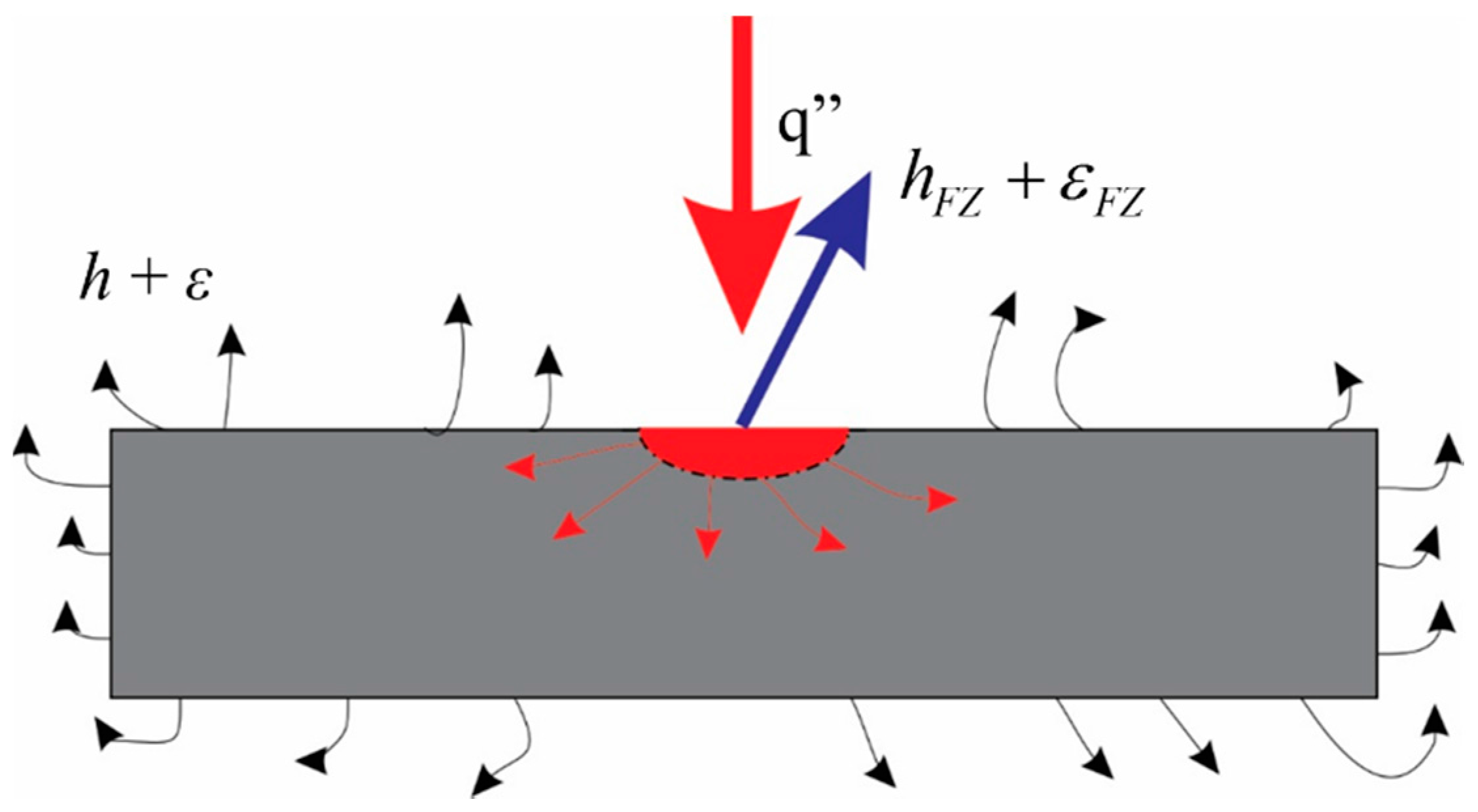
2.1. Thermal Model

Figure 1 describes the GTA welding problem which consists of a GTA torch that applies a heat flux over an aluminum plate. This GTA torch follows direction s, with velocity u. The heat input will cause a thermal gradient on the plate that could be described by the heat diffusion equation. When the welding starts, a heat loss due to the spontaneous effects of convection and radiation begins.

The GTA welding process may be expressed by the heat diffusion equation for space:

$$\frac{\partial }{\partial x}\left(\lambda (T)\frac{\partial T}{\partial x}\right)+\frac{\partial }{\partial y}\left(\lambda (T)\frac{\partial T}{\partial y}\right)+\frac{\partial }{\partial z}\left(\lambda (T)\frac{\partial T}{\partial z}\right)=\rho \frac{\partial H(T)}{\partial t},$$

(1)

where x, y and z are the Cartesians coordinates, T the temperature, λ the thermal conductivity, $\rho$ the density. The enthalpy function H is defined as:

$$H={\displaystyle \int C}dT+fL,$$

(2)

where C is the specific heat, L the latent heat and f is the Heaviside step function defined as a function of the melting temperature, T_m:

$$\begin{array}{l}f(T)=1\\ f(T)=0\end{array} \begin{array}{l}T>T_m\\ T<T_m\end{array}$$

(3)

The problem analyzed is subject to the boundary conditions of convection and radiation:

$$-\lambda (T)\frac{\partial T}{\partial \eta }=h(T)\left(T-T_{\infty }\right)+\sigma \epsilon (T)\left(T^4-T_{\infty }^4\right),$$

(4)

where η is the normal direction, h the heat transfer coefficient by convection, σ the Stefan-Boltzmann constant, ε the emissivity and T_∞ the room temperature.

The following boundary condition of heat flux, q”, is applied to the area A_xy:

$$-\lambda (T)\frac{\partial T}{\partial z}=q″(x,y,t),$$

(5)

The initial condition of imposed temperature is used for the entire domain as:

$$T(x,y,z,0)=T_{\infty },$$

(6)

The solution of the temperature field is obtained through the numerical approximation of Equation (1) by using finite difference method with the implicit formulation in time. The linear system of algebraic equations is solved by using MSI (modified strongly implicit) procedure [10].

The heat flux, q(x, y) (see Figure 1) is applied to a circular region with radius r and area A_xy. It has a Gaussian distribution and releases its energy continuously over the time as it moves with a constant positive velocity u in the x direction [2]:

$$q(x,y)=\frac{3Q}{\pi \times r^2}{e}^{-3\frac{{\left(x-u\right)}^2}{r^2}}{e}^{-\frac{3y^2}{r^2}}$$

(7)

where the Q is the heat rate function estimated through BFGS inverse technique [11].

Due to the temperature gradients in the air and the gravitational field, there is an induction of natural convection currents around the sample. The Nusselt number obtained from empirical correlations of the literature [12] was used to determine the convection coefficient h.

2.2. Aluminum 6065-T5

The cooling rate analysis for the aluminum 6065-T5 is based on the experimental procedure and data from [9]. In this work, four t+ experimental conditions (2, 7, 11, and 13 ms) were tested and three experiments were carried out for each condition with the aim of assessing the repeatability of the estimated heat flux results. The t+ is the time that the electrode remains on the positive polarity on the sample. Four experimental temperatures were used to estimate the heat flux by using the BFGS technique. The welding region was limited to a part of the sample (Figure 2). This procedure was chosen in order to minimize the high noise presented in the experimental data. For further details on the GTAW aluminum 6065-T5 experimental procedure and the thermocouple location, please see Magalhães et al. [9]. The temperatures were collected from four thermocouples fixed far from the weld region. For each experiment, 482 temperature points were observed at a time interval, Δt, of 0.78 s. The welding speed was 62.5 mm/min.

In the present work, the simulations were carried out using a new mesh to enhance the previous software [9]. The Cartesian mesh is non-uniform and it has a total of 225,000 volumes. This mesh configuration maximizes the number of mesh points in the heated region (Figure 2) where the temperature gradients are higher. The melting temperature was delimited by the lowest temperature of solid-liquid transition, T_m = 615 °C [13]. The thermal properties such as thermal conductivity, emissivity, thermal diffusivity, and specific heat were taken from fitting data points of Jensen et al. [14]. Further details on the experimental procedure, experimental data, and numerical code methodology can be seen in Magalhães et al. [9].

2.3. Stainless Steel AISI 304L

The GTA welding experiments on the stainless steel AISI 304L were described elsewhere [15]. In those experiments, nine experimental conditions were tested. The experimental conditions were based on the Taguchi robust project varying the electrode angle, arc length, current, shielding gas, and bead width. A Taguchi optimal experiment was performed. The optimal case presented an electrode angle of 30°, shielding gas of Ar + 25% He, current of 102 A, the voltage of 10.8 V, and bead width of 4 mm. The temperatures were collected in a time interval of 0.38 s and a total of 146 points. Further details on the thermocouple positioning and experimental apparatus can be seen in Lima e Silva et al. [15].

This work used the optimal experiment temperature data in order to analyze the heat transfer process on the stainless steel AISI 304L. For this case, a non-uniform 735,000-volume mesh was applied. Although the mesh size is different for the aluminum case, a mesh refinement test was done for both cases. As the welding region for the stainless steel was much bigger than for the aluminum case, a more refined mesh was used for stainless steel in order to present the results. However, the size did not affect the results. In addition, the mesh was built in order to present the same refinement on the heated region for both cases. The melting temperature, T_m = 1400 °C was obtained from International [16]. The thermal conductivity and thermal diffusivity curves were obtained from fitting data points in Touloukian et al. [17]. The AISI 304L emissivity curve was also obtained from fitting data points presented by Roger et al. [18].

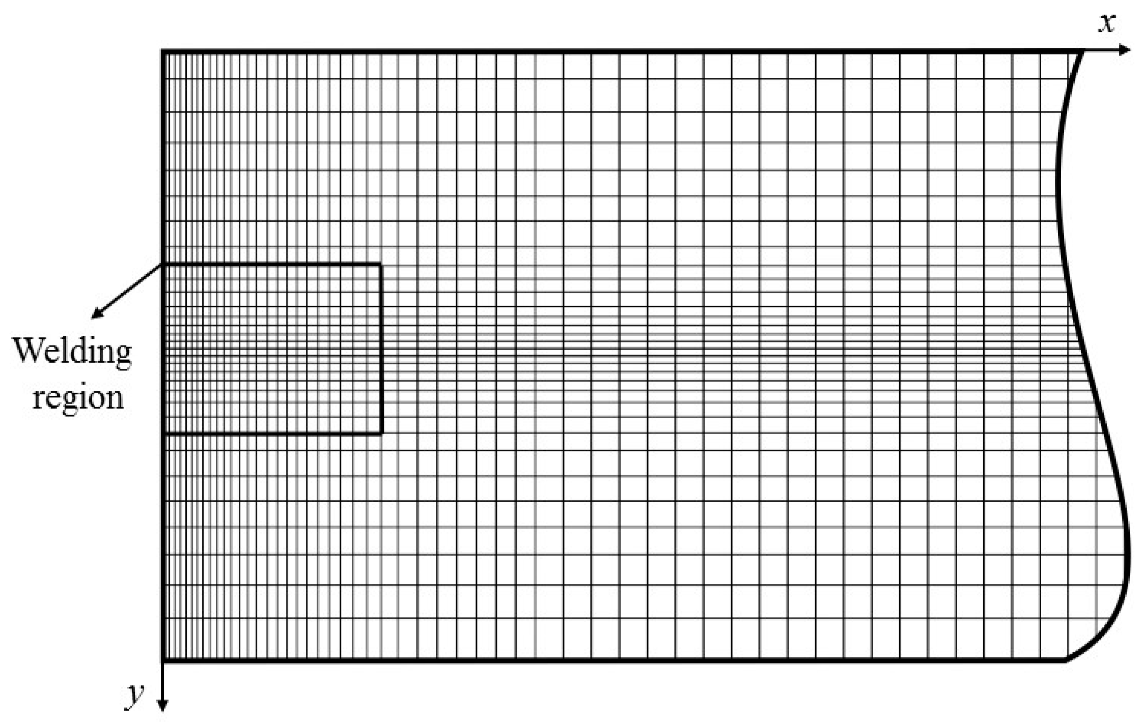
2.4. Numerical Analysis

The cooling rate analysis considered three conditions: the heat loss by convection and radiation on the fusion zone (FZ), the heat diffusion on the plate and the heat loss by convection and radiation of the heated plate. Figure 3 presents the scheme representation of the analysis performed. The blue color represents the heat loss by convection and radiation in the FZ; the black arrows are the heat loss by convection and radiation in the sample.

3. Results and Discussion

3.1. Aluminum 6065 T5

Figure 4 presents a comparison between the temperature signals measured by thermocouples T₁, T₂, T₃, and T₄. The respective numerical temperature was calculated from the previously-developed C++ code [9] for the welding conditions t+ = 2 ms, t+ = 7 ms, t+ = 11 ms, and t+ = 13 ms. It must be pointed out that the highest temperatures are obtained by the thermocouples soon after the GTA arch is turned off at t = 24 s [9].

The dimensionless Richardson number, ${Ri=Gr}_l{/Re}_l^2$, remained much higher than 1 (Ri > 1000) in all calculated points; consequently, the problem could be treated as purely free convection [12]. Thus, the empirical correlations from Bergman et al. [12] were used to calculate Nu_l, local Nusselt number and h in any position on the plate.

Figure 5 presents the average Nu profile. The average Nusselt number Nu is obtained from the arithmetic average of all Nu_l on the surface of the plate. From the analysis of Figure 5, it may be noticed that Nu increases in the first seconds of the process and it stabilizes until the arch torch is turned off. After the process, the average Nu starts to increase again. This behavior is due to the non-linear characteristics of the thermal properties for air adopted in this study. It may also be noticed that Nu is not sensitive to the positive polarity. As the average temperature increases due to the positive polarity, the Nu number remains almost at the same value for all cases studied.

Figure 6 shows the average heat transfer coefficient, h, for the four t+ welding conditions. It may be observed that the average heat transfer coefficient achieves the maximum value when the GTA torch is turned off. After this, it decreases slowly. The heat transfer coefficient by convection will return to zero when the sample reaches room temperature. It is also noticed that the heat transfer coefficient by convection increases as the positive polarity increases, however, inexpressively. When all cases were compared, the heat transfer rate by convection had not increased more the 2 W when the difference between t+ = 13 ms and t+ = 2 ms was analyzed.

The heat transfer rate lost by convection and radiation must be pointed out. As the heat transfer coefficient does not present an expressive difference from one positive polarity to another (Figure 6), the cooling rate presented almost the same values for all positive polarity conditions. Therefore, the cooling rate analysis was presented only for the experimental condition t+ = 2 ms (Figure 7). For this case, the estimated heat transfer rate using the BFGS technique was nearly 601 W. In order to compare the heat transfer rate by using constant emissivity and a heat transfer coefficient by convection, the values of ε = 0.2 for the aluminum 6065, [19] and h = 20 W/m² were used. Although the natural convection represents a large part of the overall cooling process, the heat loss by radiation significantly affects the cooling process while the GTA welding is performed. In Figure 7, for emissivity and heat transfer coefficient dependent on temperature, the heat rate loss by radiation reaches 311 W at t = 24 s while, at the same time, the heat rate loss by free convection is only 247 W. However, in this case, the heat rate loss by radiation decreases considerably when the TIG arch torch is turned off. For t = 140 s, the heat rate loss by radiation is only 13 W while by free convection is 53 W. For the case of ε = 0.2 and h = 20 W/m², which are constant, the heat rate loss by radiation reaches 143 W at t = 24 s while, at the same time, by free convection it is 340 W. These values differ significantly from the values obtained for the temperature-dependent parameters. The heat loss by radiation for t = 24 s is underestimated in 168 W, while the free convection loss is overestimated in 93 W.

When the effects of overestimation of the heat transfer coefficient and the underestimation of the radiation are combined, that is, free convection plus radiation, the overall cooling rate curve for both analyzed cases becomes similar. Figure 8 presents the cooling rate curve for the combined effects of heat transfer of temperature-dependent variables and the constant emissivity and heat transfer coefficient. The curves are similar, however, at the maximum point, t = 24 s, the cooling rate for the temperature dependent case is higher at 75 W than the case of constant parameters. Despite this difference, the cooling rate has a similar pattern for both cases (Figure 8). However, it is not recommendable to use a thermal model with constant values for emissivity and the heat transfer coefficient. In this especial case, the heat transfer by convection was overestimated and the heat transfer loss by radiation was underestimated. Nevertheless, the heat transfer model, when applied to material other than aluminum 6065 T5, could present a different result.

The fusion zone also loses heat by convection and radiation. However, those heat losses are not expressive when compared to the overall heat losses. Figure 9 presents a comparison between the heat loss by convection and radiation in the FZ and the heat loss by convection and radiation with constant emissivity, ε = 0.2, and the constant heat transfer coefficient, h = 20 W/m² is adopted. The melting point is reached when t = 3.9 s. Before this point, the weld pool is not open. Thus, the heat lost by radiation and free convection in the weld pool is nearly zero. After this point, the analyzed parameter values start to increase. Due to the higher temperature of the weld pool, the heat loss, considering the transient emissivity, is more intense. However, those losses are not as expressive when compared to the heat losses of the plate. For instance, the higher radiation occurs at t = 24 s. At this point, the GTA torch is turned off. It may be seen that, at this instant, the heat loss by radiation in the FZ reaches only 1.3 W, while the losses by free convection in the FZ are even more negligible, at 0.3W. The calculated values for a constant emissivity and heat transfer coefficient differ from the non-linear parameters. The cooling rate by convection, in this case, is higher, 0.6 W. On the other hand, the cooling rate by convection is lower, 0.4 W. If the overall heat transfer losses are considered, the model with constant variables reaches the heat loss of 1.0 W at 24 s, while the non-linear model has a heat loss of l.6 W. In spite of the significant difference between both models, the calculated values for heat losses by convection and radiation do not have a large impact on the cooling process.

Figure 10 presents the two-dimensional distribution of the heat transfer coefficient by convection for four-time steps of the simulation of the welding condition t+ = 2 ms. This figure only presents the heated part of the sample. The distribution indicates that the highest value for the heat transfer coefficient, h, follows the GTA torch movement (Figure 10a,b). It may be seen that the heat transfer coefficient by convection reaches its highest value just before the torch is turned off (Figure 10c). After 24 s, the heat transfer coefficient tends to decrease linearly until the sample reaches room temperature and the heat transfer coefficient tends to zero (Figure 10d).

After the GTA torch is turned off, the heat flux ends. Thus, the heat diffusion is evenly distributed on the plate. Consequently, all surface points tend to have the same temperature and heat transfer coefficient.

3.2. Stainless Steel

In order to accomplish a complete analysis of the cooling rate in the GTA welding process, an analysis was performed on a stainless steel AISI 304L plate. Due to its melting temperature, the stainless steel achieved a higher temperature level than the aluminum. In this case, the thermal emission has a higher impact on the cooling rate analysis. The stainless steel has a lower thermal conductivity compared to the aluminum. Therefore, the heat conduction velocity of the AISI 304L is lower than the aluminum 6065 T5. Thus, although the stainless steel welding achieves higher temperature on the welding bead, its cooling rate is lower than the welding of aluminum. Videlicet, the average temperature in the stainless steel welding is lower than in aluminum welding when the samples have the same size. This pattern is well presented in Figure 11 where the thermal field for the two sample materials is presented. It may be noticed that the center of the weld bead of the stainless steel (Figure 11a) achieves a higher temperature than the aluminum. However, due to the high thermal conduction of the aluminum 6065 T5, the temperature outside the weld bead is higher than the temperature outside the stainless steel weld bead. It may also be observed that the isothermal curves in the stainless steel present oval shapes while in the aluminum they present circular shapes. The shape is related to the welding velocity and the thermal conductivity. As the welding velocity increases the shape becomes more oval. When the thermal conductivity is high the shape becomes circular.

A comparison between the experimental temperature values for only a single thermocouple and the values obtained by the software are displayed in Figure 12. A good agreement between the curves may be observed. However, the temperature peak tends to be slightly lower when compared to the experimental temperature. This difference is related to the inherent error of the attributed values of the thermal properties. For a better precision of the calculated data at high temperatures, an estimation of the thermal conductivity and diffusivity for the stainless steel AISI 304L is required, mainly in the liquid phase. Unfortunately, there is a lack of technology development in this area. Therefore, those values are not easily found in the literature.

This fundamental pattern has an important role in the cooling analysis. Thus, the cooling rate by free convection and radiation is lower in the stainless steel than in the aluminum welding. Figure 13 presents the cooling rate by convection and radiation for the stainless steel AISI 304L welding. The cooling rate achieves the highest value at 24 s when the arc torch is turned off. At this time interval, the cooling rate by convection reaches 11.7 W, while the cooling rate lost by radiation reaches 2.8 W.

The evolution of the heat transfer coefficient for the stainless steel presented is different from the aluminum. While the aluminum reaches a heat transfer coefficient of 11.5 (W/m²K) after the arc torch is off, the stainless steel reaches only 9 (W/m²K). Figure 14 presents the evolution of the heat transfer coefficient for the stainless steel.

4. Conclusions

This paper presented an analysis of the cooling rate (lost heat transfer rate) by convection and radiation in aluminum 6065-T5 and stainless steel AISI 304L plates, under a GTA welding process from the observation of the thermal fields calculated by an in-house C++ code. The free convection effect is an important factor in heat transfer losses for both cases analyzed. However, the losses by radiation are significant in aluminum welding while the GTA torch is still on. The heat rate loss by radiation reached 311 W at the end of the welding process. On the other hand, the radiation in the stainless steel did not interfere significantly with the overall cooling rate. As a matter of fact, the external cooling, convection plus radiation, is more severe in aluminum than stainless steel.

The performed analysis represents an important step to improve the fusion and welding quality. The similarity between the experimental and calculated parameters validated and proved the efficiency of the software developed when applied to the solution of thermal problems in welding.

References

1. Dong, W.; Lu, S.; Li, D.; Li, Y. GTAW liquid pool convections and the weld shape variations under helium gas shielding. Int. J. Heat Mass Transf. 2011, 54, 1420–1431. [Google Scholar] [CrossRef]
2. Goldak, J.A.; Akhlaghi, M. Computational Welding Mechanics; Springer: New York, NY, USA, 2005. [Google Scholar]
3. Li, D.; Lu, S.; Dong, W.; Li, D.; Li, Y. Study of the law between the weld pool shape variations with the welding parameters under two TIG processes. J. Mater. Process. Technol. 2012, 212, 128–136. [Google Scholar] [CrossRef]
4. Yadaiah, N.; Bag, S. Effect of Heat Source Parameters in Thermal and Mechanical Analysis of Linear GTA Welding Process. ISIJ Int. 2012, 52, 2069–2075. [Google Scholar] [CrossRef]
5. Zareie Rajani, H.R.; Torkamani, H.; Sharbati, M.; Raygan, S. Corrosion resistance improvement in Gas Tungsten Arc Welded 316L stainless steel joints through controlled preheat treatment. Mater. Des. 2012, 34, 51–57. [Google Scholar] [CrossRef]
6. Radzievskii, V.N.; Rymar, V.I.; Besednyi, V.A.; Chernov, V.Y. Use of high-temperature vaccum welding in fabrication of the parts of centrifugal compressors. Chem. Pet. Eng. 1975, 11, 925–927. [Google Scholar] [CrossRef]
7. Gonçalves, C.V.; Carvalho, S.R.; Guimarães, G. Application of optimization techniques and the enthalpy method to solve a 3D-inverse problem during a TIG welding process. Appl. Therm. Eng. 2010, 30, 2396–2402. [Google Scholar] [CrossRef]
8. Aissani, M.; Guessasma, S.; Zitouni, A.; Hamzaoui, R.; Bassir, D.; Benkedda, Y. Three-dimensional simulation of 304L steel TIG welding process: Contribution of the thermal flux. Appl. Therm. Eng. 2015, 89, 822–832. [Google Scholar] [CrossRef]
9. Magalhães, E.D.S.; de Carvalho, S.R.; de Lima E Silva, A.L.F.; Lima E Silva, S.M.M. The use of non-linear inverse problem and enthalpy method in GTAW process of aluminum. Int. Commun. Heat Mass Transf. 2015, 66, 114–121. [Google Scholar] [CrossRef]
10. Schneider, G.E.; Zedan, M. A Modified Strongly Implicit Procedure for the Numerical Solution of Field problems. Numer. Heat Transf. Part B Fundam. 1981, 4, 1–19. [Google Scholar] [CrossRef]
11. Vanderplaats, G.N. Numerical Optimization Techniques for Engineering Design, 4th ed.; Vanderplaats Research and Development Inc.: Colorado Springs, CO, USA, 2005. [Google Scholar]
12. Bergman, T.L.; Lavine, A.S.; Incropera, F.P.; DeWitt, D.P. Fundamentals of Heat and Mass Transfer; Wiley: New York, NY, USA, 2011. [Google Scholar]
13. Toten, E.; Macknzie, D. Handbook of Aluminum—Physical Metallurgy and Process; Marcel Dekker Inc.: New York, NY, 2003. [Google Scholar]
14. Jensen, J.E.; Tuttle, W.A.; Stwart, R.B.; Brechna, H.; Prodell, A.G. Selected Cryogenic Data Notebook; Brookhaven National Laboratory: Upton, NY, USA, 1980; Vol. 2.
15. Lima e Silva, S.M.M.; Vilarinho, L.; Scotti, A.; Ong, T.; Guimaraes, G. Heat flux determination in gas-tungsten-arc welding process by using a three–dimensional model in inverse heat conduction problem. High Temp. Press. 2003, 35/36, 117–126. [Google Scholar] [CrossRef]
16. International, A. ASM Ready Reference: Thermal Properties of Metals; ASM International: Materials Park, OH, USA, 2002. [Google Scholar]
17. Touloukian, Y.S.; Kirby, R.K.; Taylor, R.E.; Desai, P.D. Volume 1: Thermal conductivity—Metallic elements and alloys. In Thermophysical Properties of Matter—The TPRC Data Series; Defense Technical Information Center: Fort Belvoir, VA, USA, 1975; p. 1595. [Google Scholar]
18. Roger, C.R.; Yen, S.H.; Ramanathan, K.G. Temperature variation of total hemispherical emissivity of stainless steel AISI 304. J. Opt. Soc. Am. 1979, 69, 1384–1390. [Google Scholar] [CrossRef]
19. Mehrtash, M.; Tari, I. A correlation for natural convection heat transfer from inclined plate-finned heat sinks. Appl. Therm. Eng. 2013, 51, 1067–1075. [Google Scholar] [CrossRef]
Figure 1. Scheme representation of the three-dimensional thermal welding process.
Applsci 07 00122 g001
Figure 2. Non-uniform Cartesian mesh applied in simulation (air view).
Applsci 07 00122 g002
Figure 3. Scheme representation of the numerical performed analysis.
Applsci 07 00122 g003
Figure 4. Evolution of the experimental and numerical temperatures for different t+ conditions.
Applsci 07 00122 g004
Figure 5. Average Nu on the plate in relation to time.
Applsci 07 00122 g005
Figure 6. Heat transfer coefficient (h) in relation to time.
Applsci 07 00122 g006
Figure 7. Cooling rate by free convection and radiation for t+ = 2 ms.
Applsci 07 00122 g007
Figure 8. Overall cooling rate for t+ = 2 ms.
Applsci 07 00122 g008
Figure 9. Heat losses in the fusion zone for t+ = 2 ms.
Applsci 07 00122 g009
Figure 10. Evolution of the heat transfer coefficient, h (W/m2K), at instants (a) 7.8 s, (b) 15.6 s, (c) 23.4 s, and (d) 39.0 s for t+ = 2.0 ms.
Applsci 07 00122 g010
Figure 11. The numerical thermal fields for GTA welding in (a) stainless steel AISI 304L and (b) aluminum 6065 T5.
Applsci 07 00122 g011
Figure 12. Numerical temperature (Tnum) and experimental temperature (Texp) for GTA welding in stainless steel AISI 304L.
Applsci 07 00122 g012
Figure 13. Overall heat transfer by convection and radiation for the GTA stainless steel welding.
Applsci 07 00122 g013
Figure 14. Evolution of the heat transfer coefficient, h (W/m2K), at instants (a) 9.5 s, (b) 19 s, (c) 28.5 s, and (d) 38.0 s for the GTA stainless steel welding.
Applsci 07 00122 g014