
A Review of Experimental Techniques for Measuring Micro- to Nano-Particle-Laden Gas Flows


Abstract
:1. Introduction
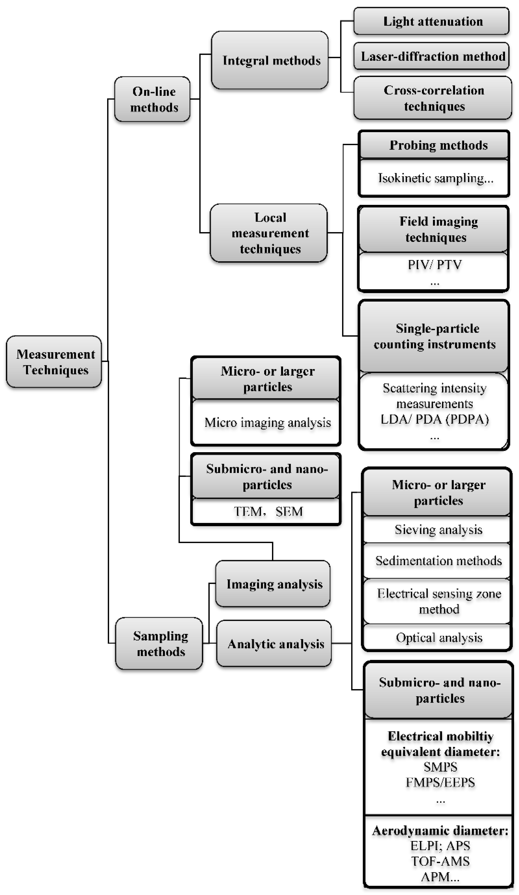
2. Classification of Experimental Methods
2.1. Parameters Used to Characterize Flows
- particle size (such as particle diameter or equivalent diameter of non-spherical particles)
- particle shape and surface area
- particle concentration or mass flow rate
- particle migration velocity and rotational velocity
- the relationship between particle size and particle velocity
2.2. Classification of Characterization Methods
2.2.1. Measurement Methods for the Dispersed Phase
2.2.2. Measuring Methods for the Carrier Phase
3. Specific Measurement Methods
3.1. Optical Particle Characterization
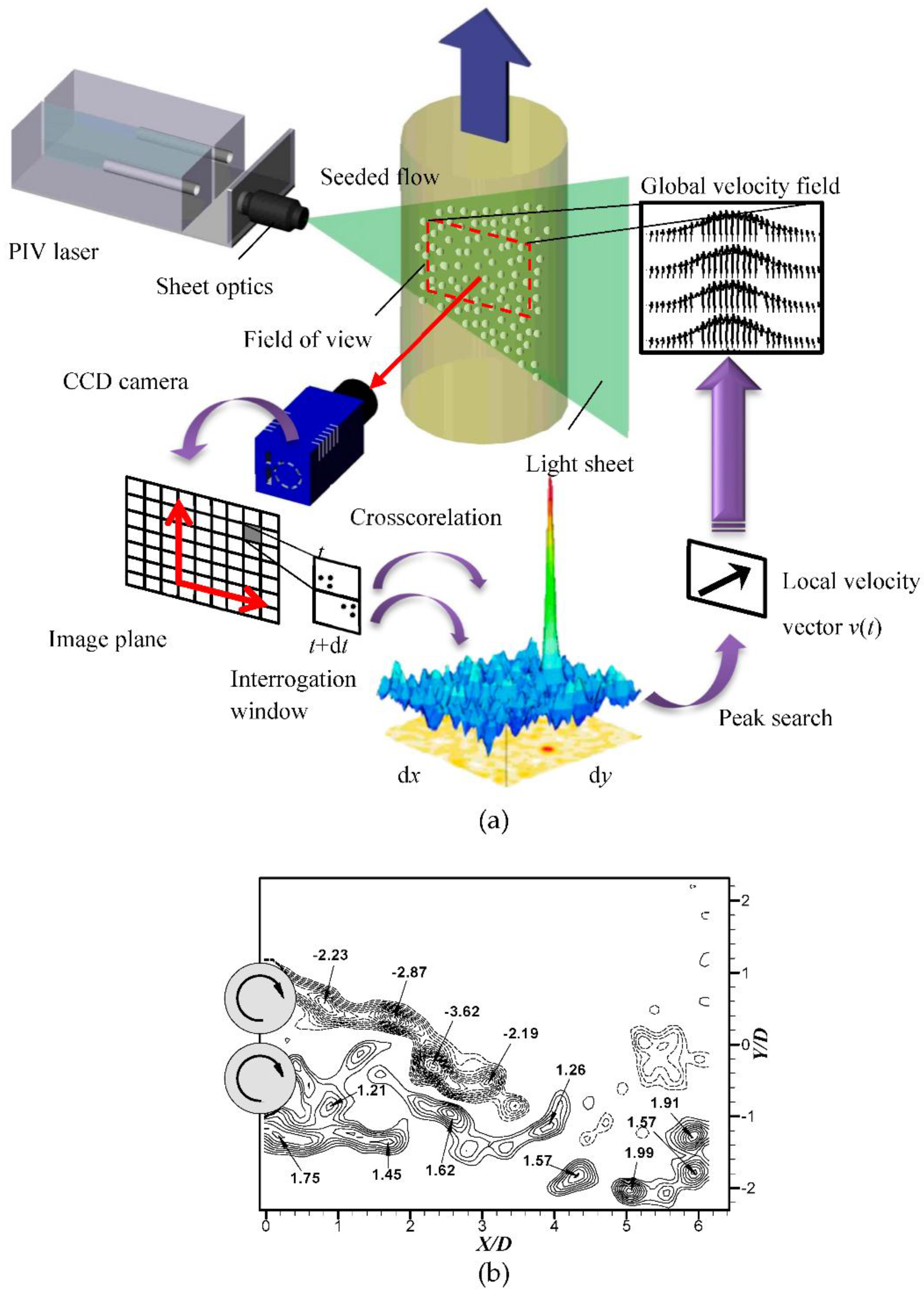
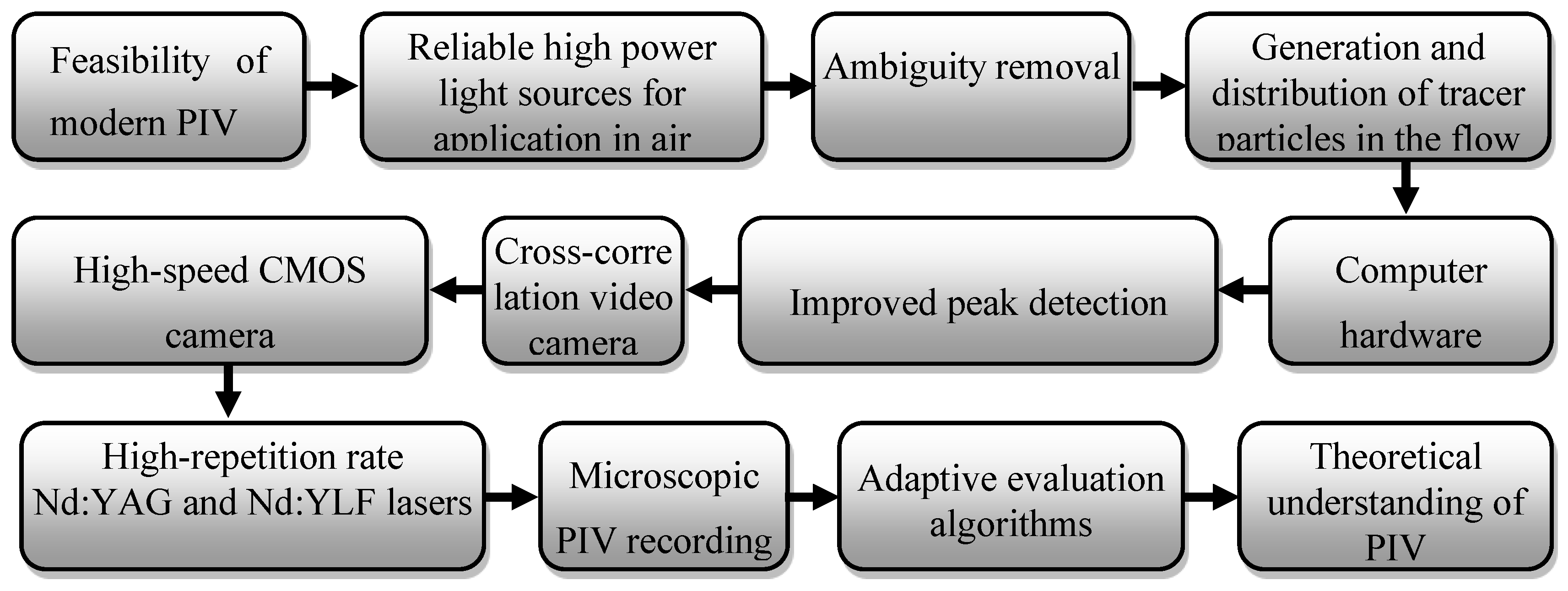
3.1.1. Particle Image Velocimetry
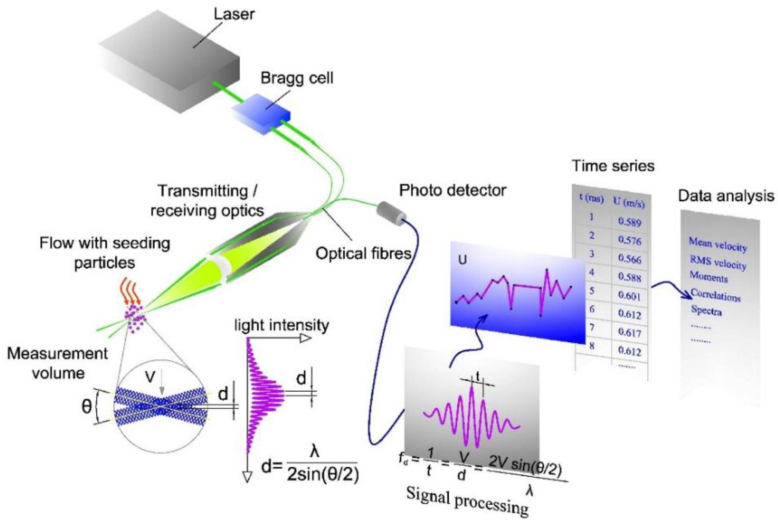
3.1.2. Laser Doppler Anemometry and the Phase Doppler Analyzer
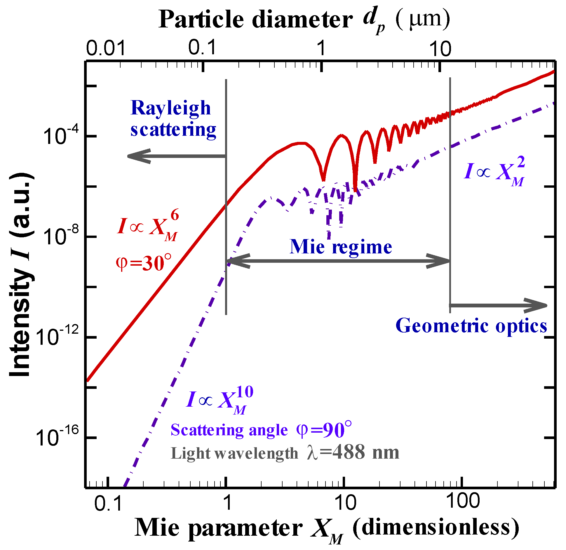
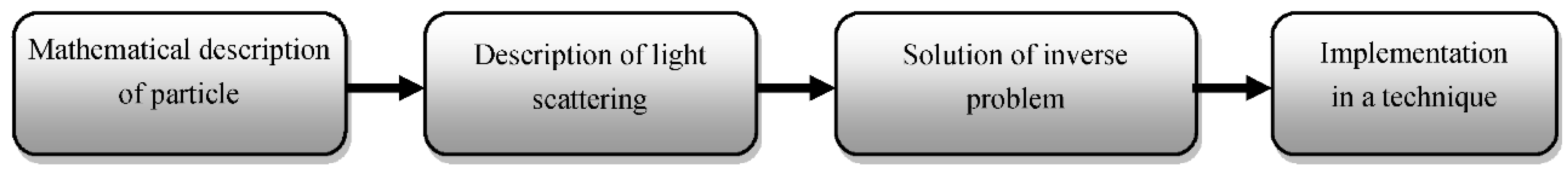
3.1.3. Scattering Intensity Measurements
3.1.4. Laser-Induced Fluorescence Techniques for Temperature and Composition Measurements
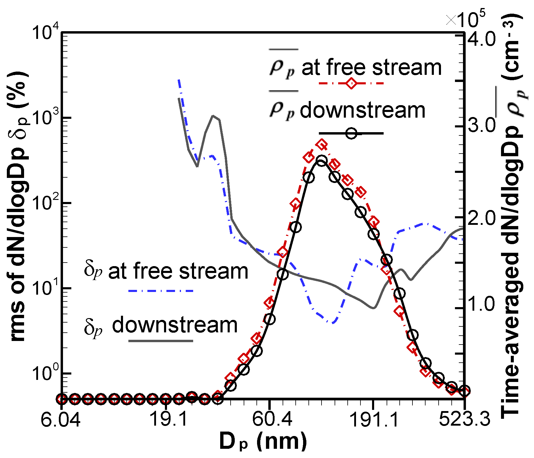
3.2. Experimental Methods for Sub-micro- and Nano-particle Laden Gas Flow
4. Conclusions
Acknowledgments
Author Contributions
Conflicts of Interest
References
- Crowe, C.T.; Sommerfeld, M.; Tsuji, Y. Multiphase Flows with Droplets and Particles; CRC Press: Boca Raton, FL, USA, 1998. [Google Scholar]
- Fuchs, N.A. On the stationary charge distribution on aerosol particles in a bipolar ionic atmosphere. Pure Appl. Geophys. 1963, 56, 185–193. [Google Scholar] [CrossRef]
- Raffel, M. Particle Image Velocimetry: A Practical Guide; Springer: New York, NY, USA, 1998; p. 216. [Google Scholar]
- Doig, I.D.; Roper, G.H. Air Velocity Profiles in Presence of Cocurrently Transported Particles. Ind. Eng. Chem. Fundam. 1967, 6, 247–256. [Google Scholar] [CrossRef]
- Hetsroni, G.; Sokolov, M. Distribution of Mass, Velocity, and Intensity of Turbulence in a Two-Phase Turbulent Jet. J. Appl. Mech. 1971, 38, 315–327. [Google Scholar] [CrossRef]
- Calzavarini, E.; Berg, T.H.V.D.; Toschi, F.; Lohse, D. Quantifying microbubble clustering in turbulent flow from single-point measurements. Phys. Fluids 2008, 20, 1569–1579. [Google Scholar] [CrossRef]
- Zhou, Y.; Yiu, M.W. Flow structure, momentum and heat transport in a two-tandem-cylinder wake. J. Fluid Mech. 2006, 548, 17–48. [Google Scholar] [CrossRef]
- Tropea, C. Optical Particle Characterization in Flows. Fluid Mech. 2011, 43, 399–426. [Google Scholar] [CrossRef]
- Albrecht, H.E.; Borys, D.I.M.; Damaschke, D.I.N.; Tropea, D.I.C. Laser Doppler and Phase Doppler Measurement Techniques; Springer: New York, NY, USA, 2003; pp. 9–26. [Google Scholar]
- Estruchsamper, D. Particle Image Velocimetry, AdrianR. J. and WesterweelJ., Cambridge University Press, The Edinburgh Building, Shaftesbury Road, Cambridge, CB2 2RU, UK. 2011. 558pp. £75. ISBN 978-0-521-44008-0. Aeronaut. J. 2012, 116, 219–220. [Google Scholar]
- Meynart, R. Mesure de champs de vitesse d’ ecoulements fluides par analyse de suites d’ images obtenues par diffusion d’ un feuillet lumineux. Ph.D. Thesis, Universite Libre de Bruxelles, Bruxelles, Belgium, 1983. [Google Scholar]
- Lauterborn, W.; Vogel, A. Modern Optical Techniques in Fluid Mechanics. Fluid Mech. 1984, 16, 223–244. [Google Scholar] [CrossRef]
- Adrian, R.J. Multi-point optical measurements of simultaneous vectors in unsteady flow—A review. Int. J. Heat Fluid Flow 1986, 7, 127–145. [Google Scholar] [CrossRef]
- Adrian, R.J. Particle-Imaging Techniques for Experimental Fluid Mechanics. Fluid Mech. 1991, 23, 261–304. [Google Scholar] [CrossRef]
- Adrian, R.J. Bibliography of Particle Velocimetry Using Imaging Methods: 1917–1995; Department of Theoretical and Applied Mechanics, University of Illinois at Urbana-Champaign: Champaign, IL, USA, 1996. [Google Scholar]
- Grant, I. Particle image velocimetry: A review. Arch. Proc. Inst. Mech. Eng. C J. Mech. Eng. Sci. 1997, 211, 55–76. [Google Scholar] [CrossRef]
- Adrian, R.J. Twenty years of particle image velocimetry. Exp. Fluids 2005, 39, 159–169. [Google Scholar] [CrossRef]
- Tu, C.X.; Bao, F.B.; Huang, L. Properties of the flow around two rotating circular cylinders in side-by-side arrangement with different rotation types. Therm. Sci. 2014, 18, 1487–1492. [Google Scholar] [CrossRef]
- Kiger, K.T.; Pan, C. PIV Technique for the Simultaneous Measurement of Dilute Two-Phase Flows. J. Fluids Eng. 2000, 122, 811–818. [Google Scholar] [CrossRef]
- Khalitov, D.A.; Longmire, E.K. Simultaneous two-phase PIV by two-parameter phase discrimination. Exp. Fluids 2002, 32, 252–268. [Google Scholar] [CrossRef]
- Sakakibara, J.; Wicker, R.B.; Eaton, J.K. Measurements of the particle-fluid velocity correlation and the extra dissipation in a round jet. Int. J. Multiph. Flow 1996, 22, 863–881. [Google Scholar] [CrossRef]
- Paris, A.; Eaton, J. Measuring velocity gradients in a particle-laden channel flow. In Proceedings of the 3rd International Workshop on PIV’99, Santa Barbara, CA, USA, 16–18 September 1999; pp. 513–518.
- Tanaka, T.; Eaton, J.K. Sub-Kolmogorov resolution partical image velocimetry measurements of particle-laden forced turbulence. J. Fluid Mech. 2010, 643, 177–206. [Google Scholar] [CrossRef]
- Balachandar, S.; Eaton, J.K. Turbulent Dispersed Multiphase Flow. Fluid Mech. 2010, 42, 111–133. [Google Scholar] [CrossRef]
- Bauckhage, K.; Floegel, H. Simultaneous measurement of droplet size and velocity in nozzle sprays. In Proceedings of the 2nd International Symposium on Applications of Laser Anemometry to Fluid Mechanics, Lisbon, Portugal, 2–5 July 1984; pp. 18.1.1–18.1.6.
- Saffman, M.; Buchhave, P.; Tanger, H. Simultaneous measurement of size, concentration and velocity of spherical particles by a laser Doppler method. In Proceedings of the 2nd International Symposium on Applications of Laser Anemometry to Fluid Mechanics, Lisbon, Portugal, 2–5 July 1984.
- Bachalo, W.D.; Houser, M.J. Phase/Doppler Spray Analyzer for Simultaneous Measurements of Drop Size and Velocity Distributions. Opt. Eng. 1984, 23, 583–590. [Google Scholar] [CrossRef]
- FlÖgel, H.H. Untersuchung von Teilchengeschwindigkeit und TeilchengrÖße mit einem Laser-Doppler-Anemometer. Ph.D. Thesis, Universität Bermen, Bermen, Germany, 1981. [Google Scholar]
- Saffman, M. The use of polarized light for optical particle sizing. In Proceedings of the 3rd International Symposium on Applications of Laser Anemometry to Fluid Mechanics, Lisbon, Portugal, 7–9 July 1986; p. 18-2.
- Sankar, S.V.; Inenaga, A.S.; Bachalo, W.D. Trajectory Dependent Scattering in Phase Doppler Interferometry: Minimizing and Eliminating Sizing Errors. In Proceedings of the 6th International Symposium on Applications of Laser Anemometry to Fluid Mechanics, Lisbon, Portugal, 20–23 July 1992; p. 12.2.
- Gréhan, D.G.; Gouesbet, G.; Naqwi, D.A.; Durst, F. Particle Trajectory Effects in Phase Doppler Systems: Computations and experiments. Part. Part. Syst. Charact. 1993, 10, 332–338. [Google Scholar] [CrossRef]
- Albrecht, H.E.; Wenzel, M.; Borys, M. Influence of the Measurement Volume on the Phase Error in Phase Doppler Anemometry. Part 2: Analysis by extension of geometrical optics to the laser beam; Refractive mode operation. Part. Part. Syst. Charact. 1996, 13, 18–26. [Google Scholar] [CrossRef]
- Xu, T.; Tropea, C. Improving the Performance of Two-Component Phase Doppler Anemometers. Meas. Sci. Technol. 1999, 5, 969–975. [Google Scholar] [CrossRef]
- Frackowiak, B.; Tropea, C. Fluorescence modeling of droplets intersecting a focused laser beam. Opt. Lett. 2010, 35, 1386–1388. [Google Scholar] [CrossRef] [PubMed]
- Frackowiak, B.; Tropea, C. Numerical analysis of diameter influence on droplet fluorescence. Appl. Opt. 2010, 49, 2363–2370. [Google Scholar] [CrossRef] [PubMed]
- Castanet, G.; Lavieille, P.; Lebouché, M.; Lemoine, F. Measurement of the temperature distribution within monodisperse combusting droplets in linear streams using two-color laser-induced fluorescence. Exp. Fluids 2003, 35, 563–571. [Google Scholar] [CrossRef]
- Castanet, G.; Delconte, A.; Lemoine, F.; Mees, L.; Gréhan, G. Evaluation of temperature gradients within combusting droplets in linear stream using two colors laser-induced fluorescence. Exp. Fluids 2005, 39, 431–440. [Google Scholar] [CrossRef]
- Maqua, C.; Depredurand, V.; Castanet, G.; Wolff, M.; Lemoine, F. Composition measurement of bicomponent droplets using laser-induced fluorescence of acetone. Exp. Fluids 2007, 43, 979–992. [Google Scholar] [CrossRef]
- Tu, C.X. Research on the Nanoparticles Cogulation and Dispersion in Shear Layers and the Related Experimental Methods; Zhejiang University: Hangzhou, China, 2015. [Google Scholar]
- Yeh, C.N.; Kosaka, H.; Kamimoto, T. A fluorescence/scattering imaging technique for instantaneous 2D measurements of particle size distribution in a transient spray. In Proceedings of the 3rd Congress Optical Partical Sizing, Yokohama, Japan, 23–26 August 1993; pp. 355–361.
- Jermy, M.C.; Greenhalgh, D.A. Planar dropsizing by elastic and fluorescence scattering in sprays too dense for phase Doppler measurement. Appl. Phys. B 2000, 71, 703–710. [Google Scholar] [CrossRef]
- Domann, R.; Hardalupas, Y. Spatial distribution of fluorescence intensity within large droplets and its dependence on dye concentration. Appl. Opt. 2001, 40, 3586–3597. [Google Scholar] [CrossRef] [PubMed]
- Domann, R.; Hardalupas, Y. A Study of Parameters that Influence the Accuracy of the Planar Droplet Sizing (PDS) Technique. Part. Part. Syst. Charact. 2001, 18, 3–11. [Google Scholar] [CrossRef]
- Barrero, A.; Loscertales, I.G. Micro- and Nanoparticles via Capillary Flows. Fluid Mech. 2007, 39, 89–106. [Google Scholar] [CrossRef]
- Lin, J.-Z.; Huang, L.-Z. Review of some researches on nano-and submicron Brownian particle-laden turbulent flow. J. Hydrodyn. Ser. B 2012, 24, 801–808. [Google Scholar] [CrossRef]
- Yu, M.; Lin, J. Nanoparticle-laden flows via moment method: A review. Int. J. Multiph. Flow 2010, 36, 144–151. [Google Scholar] [CrossRef]
- Zhu, J.; Qi, H.; Wang, J. Nanoparticle dispersion and coagulation in a turbulent round jet. Int. J. Multiph. Flow 2013, 54, 22–30. [Google Scholar]
- Yi, S.H; Tian, L.; Zhao, Y.; He, L. The new advance of the experimental research on compressible turbulence based on the NPLS technique. Adv. Mech. 2011, 41, 379–390. [Google Scholar]
- Tu, C.; Zhang, J. Nanoparticle-laden gas flow around a circular cylinder at high Reynolds number. Int. J. Numer. Methods Heat Fluid Flow 2014, 24, 1782–1794. [Google Scholar] [CrossRef]
- Wang, S.C.; Flagan, R.C. Scanning electrical mobility spectrometer. Aerosol Sci. Technol. 1990, 20, 1485–1488. [Google Scholar] [CrossRef]
- Tu, C.X.; Zhang, J.A. Characteristic distribution of submicron and nano-particles laden flow around circular cylinder. Therm. Sci. 2012, 16, 1386–1390. [Google Scholar] [CrossRef]
- Wiedensohler, A. An approximation of the bipolar charge distribution for particles in the submicron size range. J. Aerosol Sci. 1988, 19, 387–389. [Google Scholar] [CrossRef]
- Hoppel, W.A.; Frick, G.M. Ion—Aerosol Attachment Coefficients and the Steady-State Charge Distribution on Aerosols in a Bipolar Ion Environment. Aerosol Sci. Technol. 1986, 5, 1–21. [Google Scholar] [CrossRef]
- Knutson, E.O.; Whitby, K.T. Aerosol classification by electric mobility: Apparatus, theory, and applications. J. Aerosol Sci. 1975, 6, 443–451. [Google Scholar] [CrossRef]
- Agarwal, J.K.; Sem, G.J. Generating submicron monodisperse aerosols for instrument calibration. TSI Q. 1978, 4, 3–8. [Google Scholar]
- Winklmayr, W.; Reischl, G.P.; Lindner, A.O.; Berner, A.; Winklmayr, W.; Reischl, G.P.; Lindner, A.O.; Berner, A. A new electromobility spectrometer for the measurement of aerosol size distributions in the size range from 1 to 1000 nm. J. Aerosol Sci. 1991, 22, 289–296. [Google Scholar] [CrossRef]
- He, M.; Marzocca, P.; Dhaniyala, S. A new high performance battery-operated electrometer. Rev. Sci. Instrum. 2007, 78, 105103. [Google Scholar] [CrossRef] [PubMed]
- Tammet, H.; Mirme, A.; Tamm, E. Electrical aerosol spectrometer of Tartu University. J. Aerosol Sci. 1998, 29, 315–324. [Google Scholar] [CrossRef]
- Keskinen, J.; Pietarinen, K.; Lehtimäki, M. Electrical low pressure impactor. J. Aerosol Sci. 1992, 23, 353–360. [Google Scholar] [CrossRef]
- Lee, B.P.; Li, Y.J.; Flagan, R.C.; Lo, C.; Chan, C.K. Sizing Characterization of the Fast-Mobility Particle Sizer (FMPS) Against SMPS and HR-ToF-AMS. Aerosol Sci. Technol. 2013, 47, 1030–1037. [Google Scholar] [CrossRef]
- Asbach, C.; Kaminski, H.; Fissan, H.; Monz, C.; Dahmann, D.; Mülhopt, S.; Paur, H.R.; Kiesling, H.J.; Herrmann, F.; Voetz, M. Comparison of four mobility particle sizers with different time resolution for stationary exposure measurements. J. Nanopart. Res. 2009, 11, 1593–1609. [Google Scholar] [CrossRef]
- Kumar, P.; Robins, A.; Vardoulakis, S.; Britter, R. A review of the characteristics of nanoparticles in the urban atmosphere and the prospects for developing regulatory controls. Atmos. Environ. 2010, 44, 5035–5052. [Google Scholar] [CrossRef]


| Measurement Principle | Measured Quantity | Technique |
|---|---|---|
| Imaging | Velocity, particle size, shape | PIV/PTV, shadowgraphy, glare-point separation |
| Light intensity, light intensity ratio | Particle size, temperature, chemical composition | Extinction/absorption, modulation depth, Mie/LIF intensity ratio, dual band/three band LIF (laser-induced fluorescence) |
| Interferometry | velocity, particle size, refraction index/temperature | LDA, PDA, ILIDS (interferometric laser imaging for droplet size)/IPI (interferometric particle imaging), diffraction, rainbow refractometry, holography |
| Time shift | Particle size, velocity | The flying time, pulse displacement, time-shift technique |
| Pulse delay | Particle size, temperature | Femtosecond laser method |
| Raman scattering | Temperature, species concentration | Raman spectroscopy |
| Times | Authors | Reference |
|---|---|---|
| Before 1990 | Lauterborn and Vogel (1984) [12] Adrian (1986, 1991) [13,14] | “Modern optical techniques in fluid mechanics”, Ann. Rev. Fluid Mech., vol. 16, no. 16, pp. 223–244, 1984. “Multi-point optical measurements of simultaneous vectors in unsteady flow—a review”, Int. Journal of Heat and Fluid Flow, vol. 7, no. 2, pp. 127–145, 1986. “Particle-imaging techniques for experimental fluid mechanics”, Ann. Rev. Fluid Mech., vol. 23, no. 23, pp. 261–304, 1991. |
| In the 1990s | Adrian (1996) [15] Grant (1997) [16] | Bibliography of particle image velocimetry using imaging methods: 1917–1995, TAM Report 817, UILU-ENG-96-6004, University of Illinois (USA), 1996. “Particle image velocimetry: a review”, Proc. Inst. Mech. Eng. C, vol. 211, no. 1, pp. 55–76, 1997. |
| After 2000 | Adrian (2005) [17] | “Twenty years of particle image velocimetry”, Exp. Fluids, vol. 39, no. 2, pp. 159–169, 2005. |
| Physical Constants | Definition | Value | Units |
|---|---|---|---|
| e | elementary charge units | e = 1.60217733 × 10⁻¹⁹ | C |
| Dielectric constant | (F/m) | ||
| K | Boltzmann’s constant | K = 1.380658 × 10⁻²³ | (J/k) |
| ion mobility ratio |
© 2017 by the authors. Licensee MDPI, Basel, Switzerland. This article is an open access article distributed under the terms and conditions of the Creative Commons Attribution (CC BY) license ( http://creativecommons.org/licenses/by/4.0/).
Share and Cite
Tu, C.; Yin, Z.; Lin, J.; Bao, F. A Review of Experimental Techniques for Measuring Micro- to Nano-Particle-Laden Gas Flows. Appl. Sci. 2017, 7, 120. https://doi.org/10.3390/app7020120
Tu C, Yin Z, Lin J, Bao F. A Review of Experimental Techniques for Measuring Micro- to Nano-Particle-Laden Gas Flows. Applied Sciences. 2017; 7(2):120. https://doi.org/10.3390/app7020120
Chicago/Turabian StyleTu, Chengxu, Zhaoqin Yin, Jianzhong Lin, and Fubing Bao. 2017. "A Review of Experimental Techniques for Measuring Micro- to Nano-Particle-Laden Gas Flows" Applied Sciences 7, no. 2: 120. https://doi.org/10.3390/app7020120
APA StyleTu, C., Yin, Z., Lin, J., & Bao, F. (2017). A Review of Experimental Techniques for Measuring Micro- to Nano-Particle-Laden Gas Flows. Applied Sciences, 7(2), 120. https://doi.org/10.3390/app7020120