A Three-Phase Heuristic for Optimizing Truck-Drone Collaborative Delivery

Abstract

Truck-drone collaborative delivery has attracted increasing attention as an effective means to enhance flexibility and efficiency in complex distribution systems. However, the resulting Vehicle Routing Problem with Drones (VRPD) is NP-hard, and existing heuristics often struggle to balance solution quality and computational efficiency, especially in large-scale and multi-trip settings. To address these challenges, this paper proposes a Structure-Guided Adaptive Large Neighborhood Search (S-ALNS) framework for truck-drone collaborative routing. The proposed approach explicitly exploits problem-specific structural characteristics through a three-phase solution process. First, balanced initial truck routes are constructed using customer clustering. Second, a structured split-based heuristic reallocates suitable customers from truck routes to a drone service. Third, the solution is further refined within an improved ALNS framework, where a structure-guided repair mechanism based on dynamic programming is introduced to efficiently handle batch customer insertions under coupled capacity and feasibility constraints. Extensive computational experiments on instances of varying scales show that S-ALNS consistently produces near-optimal solutions for small-scale instances used for validation. For medium- and large-scale instances, S-ALNS significantly outperforms classical heuristics, including simulated annealing and a standard ALNS baseline, in terms of solution quality while maintaining competitive in computational efficiency. These results demonstrate the effectiveness of incorporating the problem structure into Adaptive Large Neighborhood Searches for complex truck-drone routing problems.

1. Introduction

Advances in unmanned aerial vehicle (UAV) platforms, learning-based decision systems, and autonomous control technologies have significantly expanded the range of practical UAV applications, including to goods delivery, environmental monitoring, and emergency response. In recent years, their adoption within the logistics industry has been particularly noteworthy. In December 2013, Amazon CEO Jeff Bezos unveiled the world’s first commercial drone delivery initiative, Amazon Prime Air, which subsequently stimulated similar efforts by companies such as Alibaba, Google, DHL, UPS, and SF Express [1,2,3,4,5]. More recently, during the COVID-19 pandemic [6], drones demonstrated substantial operational value by enabling contactless and time-critical deliveries, further accelerating the commercialization of drone-assisted logistics systems.

Despite these advances, the large-scale deployment of drones in logistics remains constrained by limited battery capacity, restricted payload, and short operational range. As a result, drones alone cannot efficiently serve all customers in last-mile delivery. Integrating trucks and drones into a coordinated delivery system has therefore emerged as a promising paradigm to exploit the complementary strengths of both modes [7]. In such systems, trucks act as mobile depots with substantial carrying capacity, while drones provide fast and flexible access to customers located in remote or congested areas. A growing body of research has demonstrated that truck-drone collaboration can significantly improve delivery efficiency and reduce operational costs in last-mile logistics.

Murray and Chu [8] first formalized this concept through the Flying Sidekick Traveling Salesman Problem (FSTSP), which was later extended to multi-truck scenarios under the framework of the Vehicle Routing Problem with Drones (VRPD) [9,10]. Most existing VRPD studies are built upon specific operational assumptions, such as restricting each drone to serve at most one customer per trip or enforcing predefined truck-drone synchronization modes (e.g., serial, parallel, or fully synchronized operations). These assumptions primarily reflect different operational policies, regulatory requirements, and managerial preferences, rather than constituting inherent oversimplifications of real-world logistics systems. For example, one-package-per-trip drone operations remain prevalent in commercial practice due to payload limitations, energy constraints, and handling considerations, while alternative synchronization schemes correspond to distinct safety and scheduling policies. Nevertheless, such assumptions inevitably restrict the feasible solution space and may hinder the exploration of more flexible coordination patterns, particularly in large-scale truck-drone routing scenarios involving multiple vehicles and repeated drone trips.

From a computational standpoint, the VRPD is an NP-hard problem. Exact solution methods, including branch-and-bound and branch-and-cut algorithms [11,12,13], are capable of producing optimal solutions for small- to medium-sized instances but quickly become computationally intractable as the problem scale increases. As a result, heuristic and metaheuristic approaches have been widely adopted [14,15,16]. Most existing heuristics follow a truck-first, drone-second construction paradigm, which may introduce structural rigidity and limit solution quality in settings with multiple trucks, multiple drones, and repeated drone operations.

Motivated by the aforementioned challenges, this paper investigates the problem of minimizing the total operational time of a multi-truck, multi-drone delivery system (mVRPD). A Mixed-Integer Linear Programming (MILP) model is formulated to characterize coordinated routing and scheduling decisions between trucks and drones, and a hybrid solution framework based on Adaptive Large Neighborhood Search (ALNS) is proposed. The framework is structured into three sequential phases. First, an initial set of truck routes is generated using a fleet-size-aware clustering strategy. Second, customers suitable for drone service are selectively reassigned from truck routes according to time-saving criteria, and the corresponding drone launch and recovery points are jointly optimized. Third, the resulting solution is further refined through an enhanced ALNS procedure equipped with problem-specific destruction and repair operators.

The main methodological contributions of this study can be summarized as follows:

• A structured ALNS-based framework for large-scale VRPD:
  A three-phase solution framework is developed that integrates clustering-based initialization, time-saving-driven drone assignment, and ALNS-based global improvement. The proposed framework emphasizes scalable coordination and scheduling in multi-truck, multi-drone settings, rather than detailed physical modeling of drone dynamics.
• Dynamic programming-enhanced repair mechanism: To address the limitations of conventional greedy insertion heuristics—such as sensitivity to insertion order and increasing computational burden when reinserting multiple customers—a dynamic programming strategy is embedded within the ALNS repair phase. This mechanism enables batch insertion decisions and improves both solution quality and computational efficiency.

The remainder of this paper is organized as follows. Section 2 reviews the relevant literature. Section 3 formally defines the problem and presents the mathematical model. Section 4 describes the proposed solution framework in detail. Section 5 reports numerical results and managerial insights. Finally, Section 6 concludes the paper and outlines directions for future research.

2. Related Literature

The last-mile delivery problem is commonly formulated as a Vehicle Routing Problem (VRP), which aims to optimize delivery routes for a fleet of vehicles in order to minimize operational costs or improve service efficiency [17]. To enhance last-mile delivery performance, Murray and Chu [8] introduced the Flying Sidekick Traveling Salesman Problem (FSTSP), in which a truck cooperates with a drone to serve customers. In this setting, the drone is launched from the truck at one customer location and recovered at a subsequent stop. The FSTSP can be viewed as a special case of the Traveling Salesman Problem with Drones (TSPD), where a truck and one or more drones collaborate to improve delivery efficiency. Extending this cooperative paradigm to multiple trucks and drones leads to the Vehicle Routing Problem with Drones (VRPD), which constitutes the focus of this study.

The VRPD was first formally introduced by Wang et al. [10]. Subsequent studies have extended the original formulation along several dimensions, including fleet configuration, drone endurance and payload constraints; truck-drone synchronization policies; and alternative optimization objectives [9,12,16,18,19,20]. With respect to optimization objectives, most VRPD studies focus on minimizing either total operational cost [20,21,22] or total delivery completion time [10,23,24,25,26,27]. The latter objective is particularly relevant for time-sensitive last-mile logistics and is therefore adopted in this study.

Exact solution methods, which rely on mathematical programming techniques to obtain optimal solutions, are effective for small-scale VRPD instances but become computationally prohibitive as the problem size increases. For example, Wang et al. [20] investigated scenarios in which drones can perform multiple deliveries per trip and dock at dedicated hubs, solving instances with up to 13 customers and TWO hubs using a branch-and-price algorithm. Tamke and Buscher [12] proposed a branch-and-cut algorithm for VRPD variants with fixed drone ranges and time-based objectives, solving instances with up to 30 nodes. Zhen et al. [18] extended the work of Roberti and Ruthmair [28] to settings involving multiple trucks, each carrying a drone; however, their approach remained limited to instances with fewer than 15 customers due to scalability constraints. Although exact methods guarantee optimality, they suffer from inherent scalability limitations caused by the exponential growth of the solution space as the numbers of trucks, drones, and customers increase. Moreover, such approaches are generally ill-suited for dynamic logistics environments, where frequent changes in demand or operational conditions require rapid re-optimization.

Heuristic approaches have therefore been widely adopted to address larger-scale VRPD instances, offering a practical balance between solution quality and computational efficiency. Early heuristic studies often relied on simplified operational assumptions to reduce computational complexity. For instance, Wang et al. [10] ignored drone range constraints to analyze worst-case delivery time ratios between truck-only and truck-drone systems. Poikonen et al. [9] incorporated drone battery limitations and operational costs to quantify the potential time savings enabled by drone assistance. Schermer et al. [14] formulated a Mixed-Integer Linear Programming model and proposed a Variable Neighborhood Search (VNS) that allows trucks to wait for drones, solving instances with up to 50 nodes. Gonzalez-R et al. [29] applied an iterated greedy algorithm to optimize multi-customer drone trips under battery constraints, successfully solving instances with up to 250 nodes. Additional heuristic and hybrid approaches include genetic algorithms [27], two-phase heuristics with multi-trip drones [24], hybrid simulated annealing and VNS methods [15], and decomposition-based algorithms for combined pickup-and-delivery scenarios [30].

Beyond problem-specific heuristics, adaptive neighborhood-based metaheuristics have emerged as a dominant paradigm for solving large-scale and highly constrained routing problems. Adaptive Large Neighborhood Search (ALNS) provides a flexible framework that dynamically selects and weights multiple destroy and repair operators throughout the search process. Recent surveys [31,32] highlight the strong performance of ALNS in handling large-scale routing problems with heterogeneous constraints. In parallel, Adaptive Variable Neighborhood Search (AVNS) has also attracted increasing attention. Karakostas et al. [33] proposed a double-adaptive VNS framework that adapts both neighborhood structures and control parameters online, while Karakostas et al. [34] further introduced learning-enhanced AVNS schemes that improve robustness and convergence behavior.

Despite these advances, several research gaps remain. Exact methods are largely restricted to small-scale instances, while many heuristic approaches rely on restrictive operational assumptions or exhibit declining solution quality as the problem size increases. These limitations highlight the need for more robust and scalable heuristic frameworks for large-scale VRPD instances. Research on the closely related Traveling Salesman Problem with Drones (TSPD) provides valuable methodological insights for addressing these challenges. Agatz et al. [35] demonstrated that carefully designed greedy route-splitting strategies can effectively coordinate truck-drone operations and generate high-quality initial solutions. Similarly, Ha et al. [36] developed a mixed-integer programming model combined with a greedy randomized adaptive search procedure and adaptive local search, solving instances with up to 100 customers. Luo et al. [37] further showed that incorporating payload-dependent energy consumption into heuristic search procedures can substantially enhance solution realism.

Motivated by the strong empirical performance of ALNS-based approaches and inspired by the greedy construction strategies proposed in studies such as Agatz et al. [35], this paper develops a Structure-Guided Adaptive Large Neighborhood Search (S-ALNS) framework for large-scale Vehicle Routing Problems with Drones. Problem-informed greedy heuristics are first employed to construct structured initial solutions, which serve as effective starting points for the subsequent search. Building upon this foundation, the proposed S-ALNS framework integrates multi-phase coordination mechanisms, fleet-size-aware clustering strategies, and a dynamic-programming-enhanced destroy-and-repair process to address the increased decision complexity arising from multi-truck, multi-drone collaboration.

3. Problem Description

This section formally defines the Multi-Vehicle Routing Problem with Drones (mVRPD) investigated in this study, which involves coordinated operations between multiple trucks and multiple drones under time-oriented objectives. The following subsection describes the operational setting, key modeling assumptions, and main decision components of the problem. Based on this definition, a mathematical formulation is then presented to rigorously capture the integrated routing and scheduling decisions between trucks and drones.

3.1. Problem Definition

The mVRPD considered in this study involves a set of customers that must be served either by trucks or by drones operating in coordination with trucks. Trucks function as both ground delivery vehicles and mobile depots for drones, while drones are dispatched to serve selected customers and subsequently return to their associated trucks. In this system, trucks act not only as ground delivery vehicles but also as mobile depots for drones. Drones are deployed from their associated trucks, deliver parcels to designated customers, and subsequently return to the same trucks. Figure 1 illustrates a schematic representation of the mVRPD. The problem is formulated under the following assumptions:

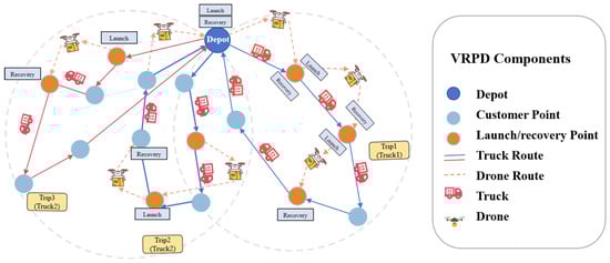
Figure 1. The VRPD model.

• Each truck is paired with exactly one drone in a one-to-one manner. The drone must return to the same truck from which it was deployed and is not allowed to dock with or be recovered by other trucks.
• Trucks and drones can perform delivery tasks independently. Drones are battery-powered, and their limited battery capacity determines the maximum feasible flight duration of each sortie. It is assumed that each drone trip starts with a fully charged battery, and battery replacement or recharging is performed upon recovery by its associated truck.
• Trucks and drones are associated with service times at customer locations. The truck service time represents the time required for loading, unloading, parking, and on-site handling activities, while the drone service time corresponds to parcel drop-off operations and is typically shorter.
• Drone deployment and recovery may take place either at the depot or at customer locations along the truck route. It is assumed that drone launch, landing, and battery replacement are handled autonomously or via integrated onboard mechanisms, and no additional personnel or handling time is explicitly modeled.
• Once a drone is dispatched from a truck or the depot, it must rendezvous with its associated truck at a customer node located downstream along the truck’s route. Drone recovery at locations not visited by the truck is not permitted.
• Trucks and drones may operate at different travel speeds; however, the ratio between their speeds is assumed to remain constant throughout the planning horizon.
• To ensure operational synchronization, if either the truck or the drone arrives earlier at a customer node designated for rendezvous, it must wait until the other arrives.

3.2. Mathematical Formulation

The problem is mathematically formulated as an MILP model using the notation presented in Table 1. The MILP formulation for the VRPD problem is introduced below:

Table 1. Notation for the VRPD with multiple trips.

Sets
V	Set of trucks, $V=\{1,2,\dots ,v\}$
$T^v$	Set of trips for truck $v\in V$, $T^v=\{1,2,\dots ,t_v\}$
$\mathcal{T}$	Set of all truck trips, $\mathcal{T}={\bigcup }_{v\in V}\{(v,t):t\in T^v\}$
C	Set of customer nodes, $C=\{1,2,\dots ,n\}$
N	Set of all nodes, $N=\left\{0\right\}\cup C\cup \{n+1\}$
$C_0$	Set of nodes including the starting depot, $C_0=\left\{0\right\}\cup C$
$C_{+}$	Set of nodes including the ending depot, $C_{+}=C\cup \{n+1\}$
$P^v$	Set of feasible drone trips associated with truck v, $P^v=\{(i,j,k)\mid i\in C_0,j\in C,k\in C_{+},t_{ij}^d+s_j^d+t_{jk}^d\le E\}$
Parameters
$Q_t$	Maximum payload capacity of a truck
$Q_d$	Maximum payload capacity of a drone
E	Maximum battery endurance of a drone (expressed as flight time)
$d_i$	Delivery demand of customer i ($i\in C$)
$t_{ij}^t$	Travel time of a truck from node i to node j
$t_{ij}^d$	Travel time of a drone from node i to node j
$\tau$	Speed ratio between drone and truck ($\tau =v_d/v_t$)
$s_i^t$	Service time of a truck at node i (including loading, unloading, and on-site handling)
$s_i^d$	Service time of a drone at node i (including parcel drop-off operations)
M	A sufficiently large positive constant
$DL$	Parameter associated with the Desrochers-Laporte subtour elimination constraints
Variables
$x_{ij}^{v,t}$	Binary, equals 1 if truck v travels from node i to node j in trip t
$y_{ijk}^{v,t}$	Binary, equals 1 if the drone of truck v in trip t is launched from i, serves customer j, and recovered at k
$T_i^{v,t}$	Arrival time of truck v at node i in trip t
$D_i^{v,t}$	Arrival time of the drone of truck v at node i in trip t
$L_i^{v,t}$	Load of truck v upon arrival at node i in trip t
$l_i^{v,t}$	Load of the drone of truck v upon arrival at node i in trip t
$w_j^{v,t}$	Binary, equals 1 if customer j is a launch and/or recovery node for the drone of truck v in trip t
$S^{v,t}$	Start time of trip t for truck v (departure from the depot)
$F^{v,t}$	Completion time of trip t for truck v (return to the depot)

Table 1. Notation for the VRPD with multiple trips.

Sets
V	Set of trucks, $V=\{1,2,\dots ,v\}$
$T^v$	Set of trips for truck $v\in V$, $T^v=\{1,2,\dots ,t_v\}$
$\mathcal{T}$	Set of all truck trips, $\mathcal{T}={\bigcup }_{v\in V}\{(v,t):t\in T^v\}$
C	Set of customer nodes, $C=\{1,2,\dots ,n\}$
N	Set of all nodes, $N=\left\{0\right\}\cup C\cup \{n+1\}$
$C_0$	Set of nodes including the starting depot, $C_0=\left\{0\right\}\cup C$
$C_{+}$	Set of nodes including the ending depot, $C_{+}=C\cup \{n+1\}$
$P^v$	Set of feasible drone trips associated with truck v, $P^v=\{(i,j,k)\mid i\in C_0,j\in C,k\in C_{+},t_{ij}^d+s_j^d+t_{jk}^d\le E\}$
Parameters
$Q_t$	Maximum payload capacity of a truck
$Q_d$	Maximum payload capacity of a drone
E	Maximum battery endurance of a drone (expressed as flight time)
$d_i$	Delivery demand of customer i ($i\in C$)
$t_{ij}^t$	Travel time of a truck from node i to node j
$t_{ij}^d$	Travel time of a drone from node i to node j
$\tau$	Speed ratio between drone and truck ($\tau =v_d/v_t$)
$s_i^t$	Service time of a truck at node i (including loading, unloading, and on-site handling)
$s_i^d$	Service time of a drone at node i (including parcel drop-off operations)
M	A sufficiently large positive constant
$DL$	Parameter associated with the Desrochers-Laporte subtour elimination constraints
Variables
$x_{ij}^{v,t}$	Binary, equals 1 if truck v travels from node i to node j in trip t
$y_{ijk}^{v,t}$	Binary, equals 1 if the drone of truck v in trip t is launched from i, serves customer j, and recovered at k
$T_i^{v,t}$	Arrival time of truck v at node i in trip t
$D_i^{v,t}$	Arrival time of the drone of truck v at node i in trip t
$L_i^{v,t}$	Load of truck v upon arrival at node i in trip t
$l_i^{v,t}$	Load of the drone of truck v upon arrival at node i in trip t
$w_j^{v,t}$	Binary, equals 1 if customer j is a launch and/or recovery node for the drone of truck v in trip t
$S^{v,t}$	Start time of trip t for truck v (departure from the depot)
$F^{v,t}$	Completion time of trip t for truck v (return to the depot)

$$\mathrm{Min}Z=\underset{v\in V,t\in T^v}{max}{F}^{v,t}$$

(1)

Subject to:

$$\sum _{v\in V}\sum _{t\in T^v}\left(\sum _{\begin{array}{c}i\in C_0\\ i\ne j\end{array}}{x}_{i,j}^{v,t}+\sum _{\begin{array}{c}i\in C_0\\ i\ne j\end{array}}\sum _{\begin{array}{c}k\in C_{+}\\ (i,j,k)\in P\end{array}}{y}_{i,j,k}^{v,t}\right)=1,\forall j\in C$$

(2)

$$\sum _{i\in C}{x}_{0,i}^{v,t}=1,\forall v\in V,t\in T^v$$

(3)

$$\sum _{j\in C_{+}}{x}_{n+1,j}^{v,t}=0,\forall v\in V,t\in T^v$$

(4)

$$\sum _{j\in C_{+}}{x}_{j,n+1}^{v,t}=1,\forall v\in V,t\in T^v$$

(5)

$$\sum _{\begin{array}{c}i\in C_0\\ i\ne j\end{array}}{x}_{i,j}^{v,t}=\sum _{\begin{array}{c}k\in C_{+}\\ k\ne j\end{array}}{x}_{j,k}^{v,t},\forall j\in C,v\in V,t\in T^v$$

(6)

$$\sum _{\begin{array}{c}j\in C\\ i\ne j\end{array}}\sum _{\begin{array}{c}k\in C_{+}\\ (i,j,k)\in P\end{array}}{y}_{i,j,k}^{v,t}\le 1,\forall i\in C_0,v\in V,t\in T^v$$

(7)

$$\sum _{\begin{array}{c}i\in C_0\\ i\ne k\end{array}}\sum _{\begin{array}{c}j\in C\\ (i,j,k)\in P\end{array}}{y}_{i,j,k}^{v,t}\le 1,\forall k\in C_{+},v\in V,t\in T^v$$

(8)

$$2y_{i,j,k}^{v,t}\le \sum _{\begin{array}{c}h\in C_0\\ h\ne i\end{array}}{x}_{h,i}^{v,t}+\sum _{\begin{array}{c}l\in C\\ l\ne k\end{array}}{x}_{l,k}^{v,t},\forall i,j\in C,k\in C_{+},v\in V,t\in T^v$$

(9)

$$y_{n+1,j,k}^{v,t}\le \sum _{\begin{array}{c}h\in C_0\\ h\ne k\end{array}}{x}_{h,k}^{v,t},\forall j\in C,k\in C_{+},v\in V,t\in T^v$$

(10)

$$\sum _{\begin{array}{c}i\in C_0\\ i\ne j\end{array}}\sum _{\begin{array}{c}k\in C_{+}\\ (i,j,k)\in P\end{array}}{y}_{i,j,k}^{v,t}\le 1-\sum _{\begin{array}{c}a\in C\\ a\ne j\end{array}}\sum _{\begin{array}{c}b\in C_{+}\\ (j,a,b)\in P\end{array}}{y}_{j,a,b}^{v,t},\forall j\in C,v\in V,t\in T^v$$

(11)

$$\sum _{\begin{array}{c}i\in C_0\\ i\ne j\end{array}}\sum _{\begin{array}{c}k\in C_{+}\\ (i,j,k)\in P\end{array}}{y}_{i,j,k}^{v,t}\le 1-\sum _{\begin{array}{c}a\in C_0\\ a\ne j\end{array}}\sum _{\begin{array}{c}b\in C\\ (a,b,j)\in P\end{array}}{y}_{a,b,j}^{v,t},\forall j\in C,v\in V,t\in T^v$$

(12)

$$D_i^{v,t}\ge T_i^{v,t}-M\left(1-\sum _{\begin{array}{c}j\in C\\ j\ne i\end{array}}\sum _{\begin{array}{c}k\in C_{+}\\ (i,j,k)\in P\end{array}}{y}_{i,j,k}^{v,t}\right),\forall i\in C,v\in V,t\in T^v$$

(13)

$$D_i^{v,t}\le T_i^{v,t}+M\left(1-\sum _{\begin{array}{c}j\in C\\ j\ne i\end{array}}\sum _{\begin{array}{c}k\in C_{+}\\ (i,j,k)\in P\end{array}}{y}_{i,j,k}^{v,t}\right),\forall i\in C,v\in V,t\in T^v$$

(14)

$$D_k^{v,t}\ge T_k^{v,t}-M\left(1-\sum _{\begin{array}{c}i\in C_0\\ i\ne k\end{array}}\sum _{\begin{array}{c}j\in C\\ (i,j,k)\in P\end{array}}{y}_{i,j,k}^{v,t}\right),\forall k\in C_{+},v\in V,t\in T^v$$

(15)

$$D_k^{v,t}\le T_k^{v,t}+M\left(1-\sum _{\begin{array}{c}i\in C_0\\ i\ne k\end{array}}\sum _{\begin{array}{c}j\in C\\ (i,j,k)\in P\end{array}}{y}_{i,j,k}^{v,t}\right),\forall k\in C_{+},v\in V,t\in T^v$$

(16)

$$T_k^{v,t}\ge T_h^{v,t}+s_h^t+t_{h,k}^t-M(1-x_{h,k}^{v,t}),\forall h\in C_0,k\in C_{+},k\ne h,v\in V,t\in T^v$$

(17)

$$D_j^{v,t}\ge D_i^{v,t}+s_i^d+t_{i,j}^d-M\left(1-\sum _{\begin{array}{c}k\in C_{+}\\ (i,j,k)\in P\end{array}}{y}_{i,j,k}^{v,t}\right),\forall j\in C,i\in C_0,i\ne j,v\in V,t\in T^v$$

(18)

$$D_k^{v,t}\ge D_j^{v,t}+s_j^d+t_{j,k}^d-M\left(1-\sum _{\begin{array}{c}i\in C_0\\ (i,j,k)\in P\end{array}}{y}_{i,j,k}^{v,t}\right),\forall j\in C,k\in C_{+},k\ne j,v\in V,t\in T^v$$

(19)

$$D_k^{v,t}-(D_j^{v,t}-t_{i,j}^d)\le E+M(1-y_{i,j,k}^{v,t}),\forall k\in C_{+},j\in C,j\ne k,v\in V,t\in T^v$$

(20)

$$L_j^{v,t}\ge L_i^{v,t}+d_j-M(1-x_{i,j}^{v,t}),\forall i\in C_0,j\in C_{+},i\ne j,v\in V,t\in T^v$$

(21)

$$L_j^{v,t}\le L_i^{v,t}+d_j+M(1-x_{i,j}^{v,t}),\forall i\in C_0,j\in C_{+},i\ne j,v\in V,t\in T^v$$

(22)

$$0\le L_i^{v,t}\le Q_t,\forall i\in N,v\in V,t\in T^v$$

(23)

$$l_j^{v,t}\ge l_i^{v,t}+d_j-M(1-\sum _{\begin{array}{c}k\in C_{+}\\ (i,j,k)\in P\end{array}}{y}_{i,j,k}^{v,t}),\forall i\in C_0,j\in C,i\ne j,v\in V,t\in T^v$$

(24)

$$l_j^{v,t}\le l_i^{v,t}+d_j+M(1-\sum _{\begin{array}{c}k\in C_{+}\\ (i,j,k)\in P\end{array}}{y}_{i,j,k}^{v,t}),\forall i\in C_0,j\in C,i\ne j,v\in V,t\in T^v$$

(25)

$$0\le l_i^{v,t}\le Q_d,\forall i\in N,v\in V,t\in T^v$$

(26)

$$S^{v,t}=T_0^{v,t},\forall v\in V,t\in T^v$$

(27)

$$F^{v,t}=T_{n+1}^{v,t},\forall v\in V,t\in T^v$$

(28)

$$S^{v,t+1}\ge F^{v,t},\forall v\in V,t=1,2,\dots ,\left|T^v\right|-1$$

(29)

$$T_0^{v,t}=S^{v,t},\forall v\in V,t\in T^v$$

(30)

$$D_0^{v,t}=S^{v,t},\forall v\in V,t\in T^v$$

(31)

$$L_0^{v,t}=0,\forall v\in V,t\in T^v$$

(32)

$$l_0^{v,t}=0,\forall v\in V,t\in T^v$$

(33)

$$x_{i,j}^{v,t}\in \{0,1\},\forall i\in C_0,j\in C_{+},j\ne i,v\in V,t\in T^v$$

(34)

$$y_{i,j,k}^{v,t}\in \{0,1\},\forall i\in C_0,j\in C,k\in C_{+},(i,j,k)\in P,v\in V,t\in T^v$$

(35)

$$T_i^{v,t},D_i^{v,t},L_i^{v,t},l_i^{v,t}\ge 0,\forall i\in N,v\in V,t\in T^v$$

(36)

$$S^{v,t},F^{v,t}\ge 0,\forall v\in V,t\in T^v$$

(37)

$$u_i^{v,t}-u_j^{v,t}+DL·x_{i,j}^{v,t}+(DL-2)x_{j,i}^{v,t}\le D-1,\forall i,j\in C,i\ne j,v\in V,t\in T^v$$

(38)

$$1+(DL-2)x_{i,n+1}^{v,t}+\sum _{\begin{array}{c}j\in C\\ i\ne j\end{array}}{x}_{j,i}^{v,t}\le u_i^{v,t}\le DL-(DL-2)x_{0,i}^{v,t}-\sum _{\begin{array}{c}j\in C\\ i\ne j\end{array}}{x}_{i,j}^{v,t},\forall i\in C,v\in V,t\in T^v$$

(39)

Routing and service assignment constraints. Objective(1) minimizes the maximum completion time among all vehicle units, defined as the time when the last unit returns to the depot. Constraint (2) guarantees that each customer is served exactly once, either by a truck or by a drone, in any trip. Constraints (3)–(5) define the start and end of each trip, requiring that every trip originates from the starting depot (node 0) and terminates at the ending depot (node n + 1) and prohibiting trucks from departing from the ending depot. Constraint (6) enforces flow conservation for trucks at each customer node within a trip.

Drone operation and coordination constraints. Constraints (7) and (8) limit drone operations by allowing at most one drone launch and one drone recovery at each truck stop within a trip. Constraint (9) ensures that if a drone trip $(i,j,k)$ is executed, the associated truck must visit both the launch node i and the recovery node k in the same trip. Constraint (10) specifies that when a drone is launched from the ending depot, the truck must visit the corresponding recovery node. Constraints (11) and (12) prohibit a node from simultaneously serving as both a drone launch and recovery point within the same trip.

Time synchronization constraints. Constraints (13)–(16) ensure temporal synchronization between trucks and drones. Specifically, constraints (13) and (14) require the drone departure time at a launch node to coincide with the truck’s arrival time, while constraints (15) and (16) enforce equality between the drone’s arrival time at a recovery node and the truck’s arrival time at that node. Constraint (17) determines the truck arrival time at each node based on its previous arrival time, service duration, and travel time. Constraints (18) and (19) define the drone arrival times at the served customer and the recovery node, accounting for service times and flight durations. Constraint (20) enforces the drone battery limitation by restricting the total flight time of each drone trip to not exceed the battery capacity E.

Capacity constraints. Constraints (21)–(23) impose truck capacity restrictions by updating the truck load along its route and ensuring it never exceeds the maximum capacity $Q_t$. Constraints (24)–(26) similarly enforce drone capacity constraints, ensuring that the drone load remains within its maximum capacity $Q_d$ throughout each drone trip.

Trip scheduling and initialization constraints. Constraints (27) and (28) link the start and finish times of each trip to the truck’s departure from and return to the depot. Constraint (29) prevents temporal overlap between consecutive trips of the same vehicle unit by enforcing that each new trip starts no earlier than the completion of the previous one. Constraints (30)–(33) initialize the departure times and loads of both trucks and drones at the starting depot. Finally, constraints (34)–(37) define the domains of the decision variables, specifying binary routing variables and non-negativity of time, load, and scheduling variables. Constraints (38) and (39) are the Desrochers–Laporte (DL) subtour elimination constraints, which prevent infeasible cycles in the truck routes for each trip.

4. VRPD Solution

This section describes the overall solution methodology developed for the VRPD. To effectively handle the coupling between truck routing, drone operations, and time-dependent constraints, we design a multi-stage heuristic framework. The core idea is to first establish a well-balanced and makespan-efficient truck routing structure, which subsequently enables effective drone deployment and large neighborhood search operations. Accordingly, the solution procedure begins with the construction of an initial truck route set, followed by drone mission generation and iterative refinement within the S-ALNS framework.

4.1. Initial Truck Route Construction

To generate a high-quality initial solution that specifically targets the minimization of the maximum completion time (makespan), we propose a truck route heuristic algorithm, as described in Algorithm 1. The algorithm first clusters customers based on geographical proximity and fleet size, then constructs and refines feasible trips within each cluster and finally schedules these trips to available trucks while balancing their workloads. The steps are detailed below.

Customer Allocation Based on Fleet Size (Algorithm 1, lines 1–6). We first calculate the theoretical minimum number of trips $m_{min}$ required to serve all customers:

$$m_{min}=⌈{\displaystyle \frac{{\sum }_{c\in C}{d}_c}{Q_t}}⌉$$

(40)

To prevent geographically remote customers from becoming bottlenecks in later scheduling stages, a sweep-based clustering strategy is adopted (Algorithm 1, lines 1–6). For each customer, the Euclidean distance to the depot $d_{0c}$ and the polar angle ${\theta }_c$ are computed (line 3). Customers are then sorted primarily by descending distance $d_{0c}$ and secondarily by ${\theta }_c$, starting from the farthest customer (line 4).

Algorithm 1 Initial Truck Route Construction

Require:  Customer set C, trucks V, capacity $Q_t$, travel times $t_{ij}^t$, service times $s_i^t$. Ensure:  Trip set $\mathcal{R}$, truck assignments, total times $\mathit{TotalTime}[1..V]$.   1: Phase 1: Customer Clustering   2: $m_{min}\leftarrow \lceil {\sum }_{c\in C}{d}_c/Q_t\rceil$   3: Compute $d_{0c}$ and ${\theta }_c$ for each customer $c\in C$   4: Sort customers by descending $d_{0c}$, then by ${\theta }_c$ from farthest   5: $K\leftarrow max(V,m_{min})$   6: Create K clusters with balanced loads (target: $\sum d_c/K$)   7: Phase 2: Trip Construction and Optimization   8: $\mathcal{R}\leftarrow Ø$   9: for each cluster $C_k$ do 10:    Sort customers in $C_k$ by ${\theta }_c$ 11:    Build trips via greedy insertion with capacity $Q_t$ 12:    Apply 2-opt to each trip in $C_k$ 13:    Merge consecutive trips if beneficial and capacity allows 14: end for 15: Phase 3: Scheduling and Load Balancing 16: for each trip $R\in \mathcal{R}$ do 17:    $T\left(R\right)\leftarrow {\sum }_{(i,j)\in R}{t}_{ij}^t+{\sum }_{i\in R}{s}_i^t$ 18: end for 19: Sort $\mathcal{R}$ by descending $T\left(R\right)$ 20: Initialize $\mathit{TotalTime}\left[v\right]\leftarrow 0$ for $v=1,\dots ,V$ 21: for each $R\in \mathcal{R}$ do 22:    Assign R to truck $v^{\ast }=arg{min}_v\mathit{TotalTime}\left[v\right]$ 23:    $\mathit{TotalTime}\left[v^{\ast }\right]\leftarrow \mathit{TotalTime}\left[v^{\ast }\right]+T\left(R\right)$ 24: end for 25: Load Balancing 26: repeat 27:    $v_{max}\leftarrow arg{max}_v\mathit{TotalTime}\left[v\right]$ 28:    $v_{min}\leftarrow arg{min}_v\mathit{TotalTime}\left[v\right]$ 29:    Try moving a trip from $v_{max}$ to $v_{min}$ 30:    Update if makespan improves and capacity permits 31: until no improvement 32: return$\mathcal{R}$, $\mathit{TotalTime}[1..V]$

The number of clusters K is set to $K=max(V,m_{min})$ as shown in line 5. If $m_{min}\le V$, we create V clusters to utilize all trucks; otherwise, $m_{min}$ clusters are created, implying truck reuse is necessary. Each cluster $C_k$ has a target load $L_{\mathrm{target}}=\left({\sum }_{c\in C}{d}_c\right)/K$. Customers are assigned greedily to the cluster with the smallest current cumulative load, balancing demand across clusters (line 6).

Trip Construction and Intra-Cluster Optimization (Algorithm 1, lines 7–15). For each cluster $C_k$, customers are processed in angular order according to ${\theta }_c$ (line 10). Trips are constructed using a greedy insertion strategy subject to the truck capacity constraint $Q_t$ (line 11). Each trip starts and ends at the depot and is finalized once no additional customer can be inserted without violating capacity.

After initial construction, two levels of intra-cluster optimization are applied. First, a 2-opt local search is performed on each trip to reduce travel distance (line 12). Second, consecutive trips within the same cluster are evaluated for possible merging (line 13). Two trips are merged if the combined demand does not exceed $Q_t$ and the merged route yields a shorter total duration than serving the trips separately. This step reduces unnecessary depot returns and improves route compactness. Specifically, for two consecutive trips $R_a$ and $R_b$, we evaluate the merged trip $R_{ab}$ and accept the merge if:

$$\sum _{c\in R_a\cup R_b}{d}_c\le Q_t\mathrm{and}T\left(R_{ab}\right)<T\left(R_a\right)+T\left(R_b\right)$$

(41)

Trip Scheduling and Inter-Truck Load Balancing (Algorithm 1, lines 15–31). Once all trips are generated, the duration of each trip R is computed as the sum of travel times and service times (lines 16–18):

$$T\left(R\right)=\sum _{(i,j)\in \mathrm{path}\left(R\right)}{t}_{ij}^t+\sum _{i\in R\setminus \{0,n+1\}}{s}_i^t$$

(42)

To minimize the makespan, trips are scheduled using a list-scheduling heuristic (lines 18–21). Trips are first sorted in descending order of $T\left(R\right)$ (line 19). Each trip is then assigned to the truck with the smallest current cumulative workload (line 22), and the corresponding total time is updated (line 23). This strategy prioritizes long trips and promotes balanced utilization across trucks.

To further reduce the makespan, an iterative load-balancing procedure is applied (lines 25–31). At each iteration, the truck with the maximum total time $v_{max}$ and the truck with the minimum total time $v_{min}$ are identified (lines 27–28). A trip is tentatively moved from $v_{max}$ to $v_{min}$ if the move reduces the maximum of their workloads and respects feasibility constraints (lines 29–30). This process continues until no improving reassignment can be found.

4.2. Drone Delivery Optimization via Split Heuristic

Building upon the initial truck routes obtained in Section 4.1, the next step is to identify customer nodes that can be more efficiently served by drones, as illustrated in Figure 2. We adapt the split heuristic proposed in [35] and [36] to the multi-trip VRPD setting. The proposed procedure, summarized in Algorithm 2, consists of three main stages: (i) feasible drone trip identification and evaluation, (ii) drone–truck substitution based on time savings, and (iii) launch and recovery node optimization.

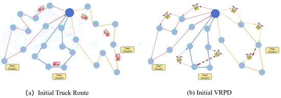
Figure 2. The initial VRPD.

Feasible drone path identification and evaluation (Algorithm 2, lines 1–17). For each initial truck route $R=[r_0,r_1,\dots ,r_m]$, the algorithm enumerates all possible drone delivery triples $(r_i,r_j,r_k)$, where $r_i$ denotes the launch node, $r_j$ the customer served by the drone, and $r_k$ the recovery node. For each candidate triple, feasibility is first checked against the drone battery constraint (lines 3–8):

$$t_{ij}^d+s_j^d+t_{jk}^d\le E,$$

(43)

where $t_{ij}^d$ and $t_{jk}^d$ are the drone flight times, $s_j^d$ is the drone service time at customer j, and E is the battery capacity.

For each feasible triple (43), the algorithm evaluates the potential benefit of substituting truck service with a drone delivery (lines 9–14). The truck travel time between launch and recovery nodes while serving customer j is computed as

$$T_{\mathrm{truck}}(i,j,k)=t_{ij}^t+s_j^t+t_{jk}^t,$$

(44)

whereas the corresponding time under drone delivery is

$$T_{\mathrm{drone}}(i,j,k)=max\left(t_{ik}^t,t_{ij}^d+s_j^d+t_{jk}^d\right).$$

(45)

The resulting time saving is then defined as

$$\mathrm{Saving}(i,j,k)=T_{\mathrm{truck}}(i,j,k)-T_{\mathrm{drone}}(i,j,k).$$

(46)

Only drone trips with positive savings are retained in the candidate set $\mathcal{D}$ (line 11).

Drone–truck substitution based on time savings (Algorithm 2, lines 18–27). All feasible drone trips in $\mathcal{D}$ are sorted in descending order of $\mathrm{Saving}(i,j,k)$ (line 17). Following this order, the algorithm sequentially attempts to replace the truck service of customer j with the corresponding drone trip $(i,j,k)$, provided that customer j has not yet been reassigned and that the launch and recovery nodes remain available (lines 19–21). This greedy replacement strategy prioritizes drone trips with the largest marginal time reductions and yields an initial set of drone trips $R_d^v$ together with the updated truck route $R_t^v$.

Launch and recovery node optimization (Algorithm 2, lines 27–53). After obtaining the initial set of drone trips $R_d^v$, we further optimize the positions of the launch node i and recovery node k for each drone trip. For recovery node optimization (lines 29–33), similarly, if the succeeding node $k+1$ of the current recovery node k is not a launch node and is not a recovery node, we attempt to shift the recovery node backward from k to $k+1$. The new drone trip becomes $(i,j,k+1)$, provided that the drone trip $(i,j,k+1)$ satisfies the battery constraint $t_{ij}^d+s_j^d+t_{j,k+1}^d\le E$ and the new time saving, $\mathrm{Saving}(i,j,k+1)$, is greater than the original, $\mathrm{Saving}(i,j,k)$. The new time saving is computed as:

$$\mathrm{Saving}(i,j,k+1)=\left[T_{\mathrm{truck}}(i,j,k)+t_{k,k+1}^t\right]-max\left(t_{i,k+1}^t,t_{ij}^d+s_j^d+t_{j,k+1}^d\right)$$

(47)

If $\mathrm{Saving}(i,j,k+1)>\mathrm{Saving}(i,j,k)$, we accept the backward shift and continue to check whether we can shift further backward (to $k+2$, etc.) until the conditions are violated or the end of the route is reached.

For launch node optimization (lines 41–45), if the preceding node $i-1$ of the current launch node i is not a recovery node and is not a launch node, we attempt to shift the launch node forward from i to $i-1$. The new drone trip becomes $(i-1,j,k)$, provided that the drone trip $(i-1,j,k)$ satisfies the battery constraint $t_{i-1,j}^d+s_j^d+t_{jk}^d\le E$ and that the new time saving, $\mathrm{Saving}(i-1,j,k)$, is greater than the original, $\mathrm{Saving}(i,j,k)$. The new time saving is computed as:

$$\mathrm{Saving}(i-1,j,k)=\left[t_{i-1,i}^t+T_{\mathrm{truck}}(i,j,k)\right]-max\left(t_{i-1,k}^t,t_{i-1,j}^d+s_j^d+t_{jk}^d\right)$$

(48)

If $\mathrm{Saving}(i-1,j,k)>\mathrm{Saving}(i,j,k)$, we accept the forward shift and continue to check whether we can shift further forward (to $i-2$, etc.) until the conditions are violated or the start of the route is reached. Through the above optimization process, we obtain the final set of drone trips and truck routes, forming an optimized VRPD solution.

Algorithm 2 Drone Delivery Optimization via Split Heuristic

Require:  Initial truck routes $\left\{R^v\right\}$, drone battery capacity E, travel times $t_{ij}^t$, $t_{ij}^d$, service times $s_i^t$, $s_i^d$. Ensure:  Optimized VRPD routes with drone deliveries.   1: Step 1: Identify feasible drone trips   2: $\mathcal{D}\leftarrow Ø$ {Set of feasible drone trips}   3: for each truck route $R=[r_0,r_1,\dots ,r_m]$ do   4:    for each possible launch node $r_i$ in R do   5:      for each possible customer node $r_j$ ($j\ne i$) in R do   6:         for each possible recovery node $r_k$ ($k>j$) in R do   7:           if $t_{ij}^d+s_j^d+t_{jk}^d\le E$ then   8:              Compute $T_{\mathrm{truck}}(i,j,k)$ and $T_{\mathrm{drone}}(i,j,k)$ using (44) and (45)   9:              $\mathrm{Saving}(i,j,k)\leftarrow T_{\mathrm{truck}}(i,j,k)-T_{\mathrm{drone}}(i,j,k)$ 10:              if $\mathrm{Saving}(i,j,k)>0$ then 11:                $\mathcal{D}\leftarrow \mathcal{D}\cup \left\{\right(i,j,k,\mathrm{Saving}(i,j,k)\left)\right\}$ 12:              end if 13:           end if 14:         end for 15:      end for 16:    end for 17: end for 18: Step 2: Sort and replace 19: Sort $\mathcal{D}$ in descending order of $\mathrm{Saving}(i,j,k)$ 20: $R_d^v\leftarrow Ø$, $R_t^v\leftarrow$ original truck routes 21: for each $(i,j,k,\mathrm{saving})$ in sorted $\mathcal{D}$ do 22:    if node j is still served by truck and $i,k$ are available then 23:      Replace truck service of j with drone trip $(i,j,k)$ 24:      Update $R_d^v$ and $R_t^v$ 25:    end if 26: end for 27: Step 3: Optimize launch and recovery nodes 28: for each drone trip $(i,j,k)$ in $R_d^v$ do 29:    while $i-1$ exists and $i-1$ is not a recovery/launch node do 30:      if $t_{i-1,j}^d+s_j^d+t_{jk}^d\le E$ then 31:         Compute $\mathrm{Saving}(i-1,j,k)$ 32:         if $\mathrm{Saving}(i-1,j,k)>\mathrm{Saving}(i,j,k)$ then 33:           Update $i\leftarrow i-1$ 34:         else 35:           break 36:         end if 37:      else 38:         break 39:      end if 40:    end while 41:    while $k+1$ exists and $k+1$ is not a launch/recovery node do 42:      if $t_{ij}^d+s_j^d+t_{j,k+1}^d\le E$ then 43:         Compute $\mathrm{Saving}(i,j,k+1)$ 44:         if $\mathrm{Saving}(i,j,k+1)>\mathrm{Saving}(i,j,k)$ then 45:           Update $k\leftarrow k+1$ 46:         else 47:           break 48:         end if 49:      else 50:         break 51:      end if 52:    end while 53: end for 54: return Optimized VRPD routes $(R_d^v,R_t^v)$

4.3. Destroy-and-Repair Algorithm Based on Adaptive Operator Selection

To enhance the quality of the initial solution and reduce the risk of convergence to local optima, this paper adopts a destroy-and-repair algorithm based on the Adaptive Large Neighborhood Search (ALNS) framework proposed in [38]. The algorithm iteratively improves the VRPD solution by alternating between destroy and repair phases: in the destroy phase, a subset of customers is removed to disrupt the current solution structure; in the repair phase, the removed customers are reinserted in a more favorable manner, thereby enabling the exploration of new solution spaces.

To reduce algorithmic complexity and accelerate convergence, several targeted simplifications are introduced relative to the standard ALNS framework. Instead of employing a large and heterogeneous set of destroy and repair operators, we retain only a small subset of problem-oriented operators that are directly compatible with the VRPD structure. Specifically, (i) destroy operations are restricted to customer-level removals, avoiding more complex route-level or sequence-based neighborhood exploration; (ii) computationally expensive repair mechanisms such as regret-k and relatedness-based insertions are eliminated and replaced by a structured three-stage insertion strategy, including drone insertion, truck insertion, and new-trip creation; and (iii) adaptive tuning of multiple ALNS parameters (e.g., cooling schedules and acceptance thresholds) is removed, while preserving only the core adaptive operator selection and weight update mechanisms.

These modifications significantly reduce the per-iteration computational complexity by limiting neighborhood enumeration and insertion evaluations, while maintaining sufficient diversification through adaptive operator selection and an adaptive destroy intensity mechanism. The overall procedure is summarized in Algorithm 3.

Operator Selection and Adaptive Mechanism. The algorithm maintains two independent weight sets for destroy operators and repair operators. At each iteration, one destroy operator and one repair operator are selected via a roulette-wheel mechanism based on their current weights. This adaptive selection strategy balances intensification and diversification by favoring operators that have performed well in the past while still allowing for exploration of alternative operators. After an operator is applied, its performance is evaluated and assigned a score ${\varphi }_i$ according to the quality of the resulting solution. Operator weights are then adaptively updated based on their accumulated scores. The scoring rules used to evaluate operator performance are summarized in Table 2.

Table 2. Operator performance scoring rules.

Symbol	Description
${\sigma }_1$	The operator produces a solution that improves the global best solution found so far.
${\sigma }_2$	The operator produces a solution that improves the current solution but does not update the global best.
${\sigma }_3$	The operator produces a solution that is inferior to the current solution but is accepted by the acceptance criterion.
${\sigma }_4$	The solution generated by the operator is rejected by the algorithm.

At the beginning of the search, all destroy and repair operators are initialized with identical weights (i.e., $w_i=w_0$ for all operators i), resulting in uniform selection probabilities in the initial phase. This neutral initialization avoids introducing operator bias before sufficient performance feedback has been accumulated. Operator weights are updated periodically rather than after every iteration. Specifically, weight updates are performed every L iterations (referred to as a segment), consistent with lines 37–39 in Algorithm 3. During each segment, the scores ${\varphi }_i$ accumulated by each operator are averaged and used to update the corresponding weights via exponential smoothing. After each update, all score accumulators are reset to zero and a new segment begins.

The weight update rule is given by

$$w_i^{\mathrm{new}}=w_i^{\mathrm{old}}·(1-\rho )+\rho ·{\displaystyle \frac{{\varphi }_i}{max\left(\varphi \right)}},$$

(49)

where $\rho \in (0,1)$ is the reaction factor controlling the sensitivity of the weights to recent performance, and $max\left(\varphi \right)$ denotes the highest average score among operators of the same type (destroy or repair) within the current segment. Based on the updated weights, the selection probability of operator i is computed as

$$P_i={\displaystyle \frac{w_i}{{\sum }_{j\in \mathcal{O}}{w}_j}}.$$

(50)

In addition to operator weights, the destroy intensity D, defined as the number of customers removed in the destroy phase, is also adaptively adjusted. Initially set to $D_0$, the value of D is dynamically updated according to recent search performance. If no improving solution is found for K consecutive iterations, the destroy intensity is increased to promote diversification; otherwise, if an improvement is observed, D is reduced to enable a finer local search. The update rule is defined as

$$D(t+1)=\left\{\begin{array}{cc}min(D_{max},D\left(t\right)+\delta ),\hfill & \mathrm{if}\mathrm{no}\mathrm{improvement}\mathrm{is}\mathrm{found}\mathrm{for}K\mathrm{consecutive}\mathrm{iterations},\hfill \\ max(D_{min},D\left(t\right)-\delta ),\hfill & \mathrm{if}\mathrm{an}\mathrm{improvement}\mathrm{is}\mathrm{found}\mathrm{in}\mathrm{the}\mathrm{current}\mathrm{iteration},\hfill \\ D\left(t\right),\hfill & \mathrm{otherwise},\hfill \end{array}\right.$$

(51)

where $D_{min}$ and $D_{max}$ denote the lower and upper bounds of the destroy intensity, and $\delta$ is the adjustment step size.

4.3.1. Destroy Operators

This paper designs four destroy operators, each targeting different characteristics of the solution for removal operations to balance the algorithm’s exploration and exploitation capabilities. All destroy operators adhere to an important principle: if a node is a drone launch or recovery point, the node itself will not be removed to maintain the basic feasibility of the route; however, when an entire drone trip is removed, its launch and recovery points are transformed into ordinary truck nodes, making them potentially removable in subsequent operations.

• Random removal: This operator randomly selects a trip (truck or drone) and removes all customer nodes within that trip. For a drone trip, after removing its service node, the associated launch and recovery points are converted to ordinary truck nodes.
• Heaviest removal: This operator calculates the total load of each truck trip (i.e., the sum of customer demands in the trip), selects the trip with the largest load, and randomly removes a certain number of customer nodes from it (the number of removals is determined by the current destroy intensity D). This operator helps break local optimal structures that may form due to capacity constraints.
• Longest time removal: This operator calculates the total time (sum of travel time and service time) of each trip (including both truck and drone trips), and selects the trip with the longest time for destruction. For a drone trip, its service node is directly removed and the launch/recovery points are converted; for a truck trip, a certain number of non-launch/recovery nodes are randomly removed. This operator directly targets the objective of minimizing the maximum completion time.
• Contribution-Based node removal: This operator evaluates the marginal contribution of each customer node to the total cost of the current solution (i.e., the reduction in cost after removing the node). It then removes nodes in descending order of their marginal contributions. This operator can precisely remove nodes that have a significant impact on cost. For each customer node $\delta$ in the current solution, we compute its marginal contribution $\Delta C\left(\gamma \right)$ as follows:

  $$\Delta C\left(\gamma \right)=t_{\mathrm{pred}\left(\gamma \right),\gamma }+t_{v,\mathrm{succ}\left(\gamma \right)}-t_{\mathrm{pred}\left(\gamma \right),\mathrm{succ}\left(\gamma \right)}$$

  (52)

  where $\mathrm{pred}\left(\gamma \right)$ and $\mathrm{succ}\left(\gamma \right)$ are the predecessor and successor nodes of $\gamma$ in the truck route, respectively, and $t_{i,j}$ is the travel time between nodes i and j. For a node v served by a drone in a trip $(i,\gamma ,k)$, its marginal contribution considers the cost difference between the current drone delivery and the alternative truck delivery. The cost of the drone trip is $T_{\mathrm{drone}}(i,v,k)$, as defined in Equation (45), and the cost of serving v by the truck (assuming insertion between i and k in the truck route) is approximated by $t_{i,\gamma }+t_{\gamma ,k}-t_{i,k}$. Thus,

  $$\Delta C\left(\gamma \right)=T_{\mathrm{drone}}(i,\gamma ,k)-(t_{i,\gamma }+t_{\gamma ,k}-t_{i,k})$$

  (53)

  Nodes with higher $\Delta C\left(v\right)$ are considered more costly to the current solution and are prioritized for removal.

4.3.2. Repair Operators

The repair operator aims to reinsert the removed customers into the current partial solution while minimizing objective deterioration and maintaining sufficient flexibility for subsequent insertions. To this end, we employ a structured repair mechanism that combines a demand-prioritized insertion order with a dynamic programming-based batch optimization procedure.

Demand-prioritized insertion order. All removed customers are first sorted in ascending order of demand. This design choice is motivated by the tightly coupled capacity, energy, and synchronization constraints inherent in the VRPD. Reinserting low-demand customers at early stages helps preserve residual truck capacity and drone payload margins, thereby increasing the feasibility of subsequent insertions. Specifically, this ordering strategy (i) mitigates premature capacity saturation on truck routes, (ii) reduces the likelihood of triggering additional trips at early stages, and (iii) improves drone assignment feasibility by maintaining sufficient payload and temporal slack for energy-constrained drone operations. Following the sorting step, customers are reinserted sequentially according to the following three-stage procedure:

• Drone insertion attempt: The algorithm first evaluates all feasible drone insertion options by enumerating admissible launch–service–recovery triplets that satisfy the drone battery constraint E. Among all feasible candidates, the option with the minimum marginal increase in objective value is selected.
• Truck insertion attempt: If no feasible drone insertion exists, the customer is considered for insertion into existing truck routes. All feasible insertion positions that satisfy the truck capacity constraint $Q_t$ are examined, and the position yielding the minimum cost increment is chosen.
• New trip creation: If neither drone nor truck insertion is feasible, a new truck trip is created for the customer. The trip is assigned to the truck with the smallest current total completion time in order to alleviate makespan imbalance across vehicle units.

Algorithm 3 Destroy-and-Repair Algorithm for the VRPD

Require:  Initial solution $R_0$, maximum iterations $I_{max}$, initial destroy intensity $D_0$, segment length L Ensure:  Best solution $R^{\ast }$   1: Initialize:$R\leftarrow R_0$, $R^{\ast }\leftarrow R_0$, $i\leftarrow 0$, $T\leftarrow T_0$   2: Initialize destroy operator weights $w_d^{\mathrm{init}}$, repair operator weights $w_r^{\mathrm{init}}$   3: Initialize destroy intensity $D\leftarrow D_0$, score accumulators ${\varphi }_d\leftarrow 0$, ${\varphi }_r\leftarrow 0$   4: while$i<I_{max}$do   5:    Adaptive Operator Selection:   6:    Select destroy operator $O_d$ using roulette wheel selection with probabilities $P_d=w_d/\sum w_d$   7:    Select repair operator $O_r$ using roulette wheel selection with probabilities $P_r=w_r/\sum w_r$   8:    Destroy Phase:   9:    $R^{\prime }\leftarrow R$ 10:    Apply the selected customer-level destroy operator $O_d$ to remove D customers from $R^{\prime }$ 11:    Update $C_{\mathrm{removed}}$ with all removed customers 12:    Repair Phase: 13:    Sort $C_{\mathrm{removed}}$ in ascending order of demand 14:    For each customer in $C_{\mathrm{removed}}$, attempt insertion in order: 15:       1. Drone insertion (minimizing cost increase, subject to battery constraint E) 16:       2. Truck insertion (minimizing cost increase, subject to capacity constraint $Q_t$) 17:       3. Create new truck trip (assigned to truck with minimum total completion time) 18:    For large batches ($|C_{\mathrm{removed}}|>K_{\mathrm{th}}$), use dynamic programming for batch optimization 19:    Post-processing: Merge consecutive trips on same truck if feasible and cost-reducing 20:    Acceptance Decision: 21:    if $\mathrm{Cos}\mathrm{t}\left(R^{\prime }\right)<\mathrm{Cos}\mathrm{t}\left(R\right)$ then 22:      $R\leftarrow R^{\prime }$ 23:      if $\mathrm{Cos}\mathrm{t}\left(R^{\prime }\right)<\mathrm{Cos}\mathrm{t}\left(R^{\ast }\right)$ then 24:         $R^{\ast }\leftarrow R^{\prime }$ 25:         Update ${\varphi }_d$ and ${\varphi }_r$ with ${\sigma }_1$ for $O_d$ and $O_r$ 26:      else 27:         Update ${\varphi }_d$ and ${\varphi }_r$ with ${\sigma }_2$ for $O_d$ and $O_r$ 28:      end if 29:    else if $\mathrm{Random}(0,1)<exp(-(\mathrm{Cos}\mathrm{t}\left(R^{\prime }\right)-\mathrm{Cos}\mathrm{t}\left(R\right))/T)$ then 30:      $R\leftarrow R^{\prime }$ 31:      Update ${\varphi }_d$ and ${\varphi }_r$ with ${\sigma }_3$ for $O_d$ and $O_r$ 32:    else 33:      Update ${\varphi }_d$ and ${\varphi }_r$ with ${\sigma }_4$ for $O_d$ and $O_r$ 34:    end if 35:    Adaptive Intensity Adjustment: 36:    Update destroy intensity D using Equation (51) 37:    Periodic Weight Update: 38:    if $imodL=0$ then 39:      Update $w_d$ and $w_r$ using exponential smoothing: $w^{\mathrm{new}}=w^{\mathrm{old}}·(1-\rho )+\rho ·{\displaystyle \frac{\varphi }{max\left(\varphi \right)}}$ 40:      Reset ${\varphi }_d\leftarrow 0$, ${\varphi }_r\leftarrow 0$ 41:    end if 42:    $i\leftarrow i+1$ 43:    $T\leftarrow T·\alpha$ {Temperature update} 44: end while 45: return$R^{*}$

Dynamic programming-based batch repair. When a large number of customers are removed simultaneously, greedy sequential insertion may lead to suboptimal or myopic decisions due to strong inter-dependencies among insertion choices. To address this issue, we introduce a dynamic programming (DP)-based batch repair mechanism, which constitutes a key component of the proposed ALNS framework. As illustrated in Figure 3, the DP procedure constructs a state table $dp\left[k\right]\left[l\right]$, where k denotes the number of customers processed and l represents the cumulative load of the current trip. State transitions explicitly model two competing decisions: inserting the next customer into the current trip (if capacity permits) or terminating the current trip and starting a new one. Each transition is associated with a corresponding marginal cost, accounting for travel time, service time, and truck assignment effects.

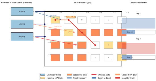
Figure 3. Dynamic programming for batch insertion optimization.

By systematically enumerating feasible transition paths and evaluating their cumulative costs, the DP procedure identifies the globally optimal insertion pattern for the batch, rather than relying on locally optimal greedy choices. This mechanism is particularly effective in scenarios where capacity saturation and trip segmentation decisions are tightly coupled, and it significantly improves the robustness and solution quality of the repair phase. Finally, after all customers have been reinserted, a post-processing step is applied. Consecutive trips assigned to the same truck are examined and merged whenever the capacity constraint is respected and the total travel time can be reduced.

4.4. Computational Complexity Analysis

This subsection analyzes the computational complexity of the proposed S-ALNS framework by examining its three major components: initial truck route construction, drone delivery optimization, and the adaptive destroy-and-repair procedure.

Initial Truck Route Construction (Algorithm 1). Let n denote the number of customers and V the number of trucks. The customer clustering phase requires sorting customers by distance and angle, resulting in a complexity of $O(nlogn)$. Trip construction within clusters is performed using greedy insertion, which in the worst case incurs $O\left(n^2\right)$ time. The subsequent 2-opt local search applied to each trip has quadratic complexity in the trip size; aggregated over all trips, this step remains bounded by $O\left(n^2\right)$. Trip scheduling and load balancing involve sorting the generated trips and iteratively reassigning them among trucks, which is polynomial in the number of trips and trucks. Overall, the computational complexity of the initialization phase is dominated by $O\left(n^2\right)$.

Drone Delivery Optimization (Algorithm 2). For a truck route containing m nodes, the enumeration of all feasible drone delivery triples $(i,j,k)$ has a worst-case complexity of $O\left(m^3\right)$. In practice, this search space is significantly reduced by restricting launch and recovery candidates based on route order and feasibility considerations, resulting in near-quadratic behavior. The subsequent launch and recovery node adjustment procedures operate in linear time with respect to the route length for each accepted drone trip. Since drone optimization is applied independently to each truck route and $m\ll n$ in typical instances, this component does not dominate the overall computational cost.

Destroy-and-Repair Algorithm (Algorithm 3). Each SA-ALNS iteration consists of a destroy phase and a repair phase. All destroy operators operate at the customer or trip level and have linear or $O(nlogn)$ complexity. The repair phase follows a structured three-stage insertion strategy. For each removed customer, evaluating feasible drone and truck insertions requires examining all admissible insertion positions, leading to a worst-case complexity of $O\left(n^2\right)$ per iteration. When a large batch of customers is removed, a dynamic programming-based batch repair mechanism is invoked. For a batch of size q, this procedure has complexity $O(q·Q_t)$, where $Q_t$ is the truck capacity, and is triggered only when q exceeds a predefined threshold. As the batch size q is controlled by the adaptive destroy intensity, the per-iteration complexity remains polynomial.

Let $I_{max}$ denote the maximum number of iterations. The overall computational complexity of the proposed algorithm is therefore bounded by $O(I_{max}·n^2)$. Importantly, the adaptive operator selection and destroy intensity adjustment mechanisms do not increase the asymptotic complexity, but instead improve practical efficiency by guiding the search toward promising regions of the solution space.

5. Computational Examples and Results

This section evaluates the performance of the proposed algorithm through three sets of computational experiments designed to assess solution quality, scalability, and robustness across different problem sizes. The first experiment focuses on small-scale instances, consisting of five randomly generated datasets with eight customer nodes each. For these instances, the performance of the proposed algorithm is benchmarked against optimal solutions obtained from the Mixed-Integer Linear Programming (MILP) formulation. Details of the instance generation procedure are provided in Section 5.1. The second experiment considers medium-scale instances with 25 and 50 customer nodes, generated using the same methodology as the small-scale cases. Algorithmic performance is again evaluated by comparison with optimal or best feasible solutions produced by the MILP solver within the specified time limits. The third experiment is designed to assess the scalability of the proposed algorithm. To this end, we employ widely used benchmark datasets, including KroA100, KroA200, and Rd400. For these large-scale instances, the obtained solutions are compared with the best-known results reported in the literature.

In all experiments, both trucks and drones operate in a two-dimensional Euclidean space. The truck speed is normalized to 1, while the drone speed is set to 2, reflecting the typical speed advantage of aerial vehicles over ground transportation. The algorithm is implemented in Python 3.9, and all computational experiments are conducted on a workstation equipped with an AMD Ryzen 7 6800H processor (3.20 GHz) and 16 GB of RAM.

5.1. Instance Generation

To comprehensively evaluate the proposed algorithm under diverse spatial conditions, we design five datasets with distinct depot locations and customer distribution patterns. These datasets cover both small-scale (eight customers) and medium-scale (25 and 50 customers) instances. All customer and depot coordinates are generated within a $100\times 100$ Euclidean space.

The five datasets are defined as follows:

• Dataset 1 (Uniform–Central): Customer nodes are uniformly distributed over the entire region, with the depot located at the center $(50,50)$.
• Dataset 2 (Uniform–Boundary): Customer nodes are uniformly distributed, while the depot is positioned at the bottom center $(50,0)$, introducing spatial asymmetry and longer access distances.
• Dataset 3 (Random–Central): Customer nodes follow a random spatial distribution, with the depot located at the center $(50,50)$.
• Dataset 4 (Annular): Customer nodes are uniformly distributed within an annular region centered at $(50,50)$, with inner and outer radii of 25 and 50, respectively.
• Dataset 5 (Clustered): Customer nodes are grouped into multiple non-overlapping clusters, each confined within a circular region of radius 12.5, while the depot is located at the center $(50,50)$.

For all datasets, customer demands are independently generated from a discrete uniform distribution on $\{1,\dots ,5\}$. Truck capacities are set such that multiple trips are required for medium-scale instances, while drone battery capacities are calibrated based on Euclidean flight distances to ensure realistic feasibility.

Unless otherwise stated, the following parameters are used consistently across all experiments. The truck cruising speed is set to 30 km/h, while the drone cruising speed is set to 60 km/h [39], reflecting typical speed settings adopted in truck-drone cooperative delivery studies. This configuration corresponds to a drone-to-truck speed ratio of approximately 2:1, which is commonly assumed in the literature to capture the higher mobility of aerial vehicles without overstating their advantage. The maximum payload capacity of each truck is 500 kg, allowing multiple delivery and pickup operations within a single route, while the maximum payload capacity of each drone is limited to 20 kg, consistent with the carrying capacity of small-scale logistics drones. The maximum allowable drone flight duration is set to 40 min per mission, representing a moderate endurance level that balances operational feasibility and system-level efficiency, as further examined in the sensitivity analysis.

For the S-ALNS framework, the maximum number of iterations is set to 3000 for small- and medium-scale instances, and increased to 5000 for large-scale benchmark instances. The maximum number of consecutive non-improving iterations is fixed at $\mathit{maxNonImprove}=100$. These settings provide a balance between solution quality and computational efficiency and are kept identical for all comparative algorithms to ensure fairness.

To further assess scalability on large-scale problems, we additionally consider well-established benchmark datasets from the literature, including KroA100, KroA200, and Rd400. These instances contain 100, 200, and 400 customer nodes, respectively, and are widely used to evaluate the performance of large-scale vehicle routing algorithms.

5.2. Experimental Results and Analysis

This subsection provides a comprehensive experimental evaluation of the proposed S-ALNS algorithm. Section 5.2.1 assesses the solution accuracy of S-ALNS by comparing its results with exact solutions. Section 5.2.2 reports a detailed performance analysis on medium-scale instances, while Section 5.2.3 presents large-scale experimental results based on the KroA and Rd400 datasets. Finally, Section 5.3 summarizes key findings and examines the robustness of the proposed algorithm. In all experiments, the S-ALNS algorithm was independently executed 10 times for each instance, and the solution with the lowest objective value was reported as the best result. A solution was regarded as equal to or better than the Gurobi solution if its objective value was less than or equal to the best feasible solution obtained by Gurobi within the prescribed time limit. Table 3, Table 4 and Table 5 summarize the experimental results. The first column, denoted as “Inst.”, adopts the notation “n.R.D”, where “n” indicates the instance index, “R” denotes the number of trucks, and “D” represents the dataset type defined in Section 5.1.

Table 3. Comparison of results for small-scale VRPD instances.

Inst	MILP		SA					ALNS					S-ALNS
	Obj	Time (s)	Best	Best%	Avg Obj	Avg%	Time (s)	Best	Best%	Avg Obj	Avg%	Time (s)	Best	Best%	Avg Obj	Avg%	Time (s)
1.1.0	222.84	671.93	241.67	8.45	241.67	8.45	0.82	222.84	0.00	222.84	0.00	0.81	222.84	0.00	222.84	0.00	0.98
1.1.1	170.79	702.71	207.53	21.51	207.53	21.51	0.75	170.79	0.00	170.79	0.00	1.07	170.79	0.00	170.79	0.00	1.01
1.1.2	168.54	1492.70	168.54	0.00	198.72	17.91	0.94	168.75	0.12	178.30	5.79	1.00	168.75	0.12	170.57	1.20	0.95
2.1.0	258.93	653.67	258.93	0.00	258.93	0.00	0.85	258.93	0.00	258.93	0.00	1.01	258.93	0.00	258.93	0.00	0.95
2.1.1	218.47	705.15	228.32	4.51	228.32	4.51	0.87	228.32	4.51	228.32	4.51	1.03	218.47	0.00	223.39	2.25	1.00
2.1.2	199.21	1051.25	209.06	4.94	238.33	19.64	0.94	209.06	4.94	249.02	25.00	1.00	199.21	0.00	221.84	11.36	1.04
3.1.0	217.93	892.46	220.67	1.26	220.67	1.26	0.86	217.93	0.00	217.93	0.00	1.02	217.93	0.00	217.93	0.00	1.03
3.1.1	172.11	2431.91	191.87	11.48	191.87	11.48	0.92	183.85	6.82	183.85	6.82	1.03	172.11	0.00	177.98	3.41	1.13
3.1.2	169.92	3600.00	196.76	15.80	215.31	26.71	0.83	178.98	5.33	212.63	25.14	1.04	170.39	0.28	178.21	4.88	1.01
4.1.0	237.41	743.19	244.42	2.95	244.42	2.95	0.91	237.41	0.00	237.41	0.00	1.05	237.41	0.00	237.41	0.00	0.94
4.1.1	185.11	1215.44	215.51	16.42	215.51	16.42	1.08	185.11	0.00	185.11	0.00	1.03	185.11	0.00	185.11	0.00	1.01
4.1.2	198.22	3600.00	199.77	0.78	216.42	9.18	0.93	199.68	0.73	215.15	8.54	1.02	199.68	0.73	205.64	3.74	1.03
5.1.0	240.36	763.29	241.17	0.34	241.17	0.34	1.11	256.15	6.57	256.17	6.57	1.00	241.17	0.34	241.17	0.34	1.17
5.1.1	205.20	709.82	206.42	0.60	206.42	0.60	0.88	221.19	7.79	221.19	7.79	1.02	205.27	0.04	206.17	0.48	1.01
5.1.2	190.74	834.56	194.87	2.17	197.81	3.71	0.89	191.91	0.61	212.02	11.16	1.18	190.94	0.10	191.56	0.43	1.03
Mean		1337.87		6.08		9.64	0.91		2.49		6.75	1.02		0.108		1.873	1.02

Table 4. Comparison of the results obtained by solving the 25-node VRPD.

Inst	MILP		SA					ALNS					S-ALNS
	Obj	Time (s)	Best	Best%	Avg Obj	Avg%	Time (s)	Best	Best%	Avg Obj	Avg%	Time (s)	Best	Best%	Avg Obj	Avg%	Time (s)
25.1.1	415.15	3600	397.21	23.58	397.21	−4.32	5.02	321.42	0.00	321.42	−22.58	5.08	321.42	0.00	321.42	−22.58	5.01
25.1.2	373.29	3600	331.80	14.23	345.97	−7.13	5.09	311.82	7.36	321.24	−13.41	5.17	296.01	0.00	296.01	−7.75	5.02
25.1.3	355.64	3600	323.52	12.16	339.93	−4.42	5.03	303.14	5.09	317.23	−10.80	5.27	288.46	0.00	299.77	−15.71	5.02
25.1.4	349.19	3600	325.09	20.13	333.07	−4.64	5.03	309.92	14.52	322.28	−7.71	6.00	270.62	0.00	287.08	−17.79	5.42
25.1.5	355.80	3600	342.76	17.56	360.58	1.34	6.03	333.70	14.46	333.66	−4.54	6.27	291.55	0.00	304.20	−14.50	5.92
25.2.1	387.84	3600	343.51	16.03	343.51	−11.43	7.14	296.04	0.00	296.04	−23.67	6.49	296.04	0.00	296.04	−23.67	5.93
25.2.2	364.66	3600	333.16	4.27	343.72	−5.74	5.82	343.36	7.46	350.39	−3.91	5.46	319.51	0.00	328.16	−10.01	5.15
25.2.3	414.3	3600	378.78	11.01	390.01	−5.86	6.26	376.07	10.22	399.25	−3.63	7.07	341.21	0.00	362.13	−12.59	6.15
25.2.4	442.1	3600	412.34	9.60	436.89	−1.18	7.35	394.27	4.80	414.77	−6.18	7.00	376.22	0.00	404.07	−8.60	6.82
25.2.5	493.62	3600	490.57	5.84	498.98	1.09	7.38	474.33	2.34	486.25	−1.49	7.04	463.49	0.00	474.75	−3.82	6.72
25.3.1	381.99	3600	359.02	38.73	359.02	−6.01	7.16	258.80	0.00	258.80	−32.25	6.89	258.80	0.00	258.80	−32.25	7.12
25.3.2	328.57	3600	266.20	2.64	295.47	−10.07	8.02	266.63	2.81	279.27	−15.00	7.87	259.35	0.00	272.98	−16.92	8.01
25.3.3	346.912	3600	279.42	4.94	294.93	−14.98	8.03	285.74	7.32	289.93	−16.43	8.06	266.26	0.00	270.18	−22.12	8.02
25.3.4	306.88	3600	275.90	14.66	284.17	−7.40	7.35	269.21	11.88	282.05	−8.09	7.05	240.62	0.00	249.75	−18.62	6.92
25.3.5	297.81	3600	296.47	15.12	301.23	1.15	7.37	268.07	4.09	277.91	−6.68	7.56	257.54	0.00	268.60	−9.81	7.24
25.4.1	382.74	3600	358.03	52.10	358.03	−6.46	7.94	235.39	0.00	235.39	−38.50	7.11	235.39	0.00	235.39	−38.50	7.28
25.4.2	270.69	3600	261.24	10.82	265.46	−1.93	7.26	242.09	2.70	244.38	−9.72	7.54	235.74	0.00	237.96	−12.09	7.02
25.4.3	268.41	3600	252.39	2.20	265.97	−0.91	7.28	259.40	5.04	259.95	−3.15	7.54	246.96	0.00	247.16	−7.92	7.00
25.4.4	287.96	3600	266.88	7.42	275.28	−4.40	7.37	261.55	5.28	268.72	−6.68	7.06	248.45	0.00	254.42	−11.65	7.02
25.4.5	301.62	3600	272.57	12.90	278.10	−7.80	5.36	276.61	14.57	282.02	−6.50	6.04	241.44	0.00	258.74	−14.22	5.35
25.5.1	273.8	3600	264.71	37.67	264.71	−3.32	6.78	192.28	0.00	192.28	−29.77	6.11	192.28	0.00	192.28	−29.77	5.71
25.5.2	204.946	3600	209.72	33.77	214.57	4.70	5.21	186.99	19.27	186.99	−8.76	5.78	156.78	0.00	161.15	−21.37	5.12
25.5.3	212.76	3600	200.68	21.83	203.16	−4.51	6.03	181.79	10.36	184.07	−13.49	6.83	164.73	0.00	169.19	−20.48	5.93
25.5.4	201.02	3600	182.82	8.12	187.93	−6.51	5.32	187.04	10.61	187.54	−6.71	5.76	169.10	0.00	172.07	−14.40	5.02
25.5.5	201.32	3600	193.88	8.65	194.96	−3.16	5.39	198.09	11.01	201.77	0.22	5.85	178.44	0.00	180.16	−10.51	5.01
Mean		3600		16.24		−4.56	6.48		6.85		−11.94	6.56		0.00		−17.22	6.20

Table 5. Comparison of the results obtained by solving the 50-node VRPD.

Inst	MILP		SA					ALNS					S-ALNS
	Obj	Time (s)	Best	Best%	Avg Obj	Avg%	Time (s)	Best	Best%	Avg Obj	Avg%	Time (s)	Best	Best%	Avg Obj	Avg%	Time (s)
50.1.1	635.50	3600	693.81	9.18	704.52	10.86	17.03	426.83	−32.84	426.83	−32.84	18.31	426.83	−32.84	426.83	−32.84	17.07
50.1.2	533.75	3600	496.21	−7.04	556.76	4.31	18.25	426.13	−20.16	447.60	−16.14	17.82	360.99	−32.37	366.40	−31.35	18.02
50.1.3	493.99	3600	487.47	−1.32	530.28	7.35	18.03	410.16	−16.97	444.22	−10.08	18.57	364.63	−26.19	392.81	−20.48	17.15
50.1.4	478.90	3600	462.72	−3.38	483.19	0.90	19.05	408.91	−14.61	422.88	−11.70	20.18	382.76	−20.07	395.77	−17.36	18.29
50.1.5	475.99	3600	457.19	−3.95	475.55	−0.09	20.50	417.48	−12.29	438.69	−7.84	19.15	398.19	−16.34	412.75	−13.29	20.40
50.2.1	684.35	3600	827.41	20.91	827.41	20.91	19.41	442.36	−35.36	442.36	−35.36	21.35	442.36	−35.36	442.36	−35.36	21.01
50.2.2	623.15	3600	605.20	−2.88	646.28	3.71	20.49	436.36	−29.98	466.36	−25.16	19.82	436.36	−29.98	456.44	−26.75	18.52
50.2.3	589.12	3600	561.54	−4.68	579.85	−1.57	22.51	509.40	−13.53	520.57	−11.64	21.18	461.56	−21.66	504.30	−14.40	20.00
50.2.4	580.78	3600	571.39	−1.62	608.82	4.83	19.57	554.03	−4.60	561.82	−3.27	21.16	458.00	−21.15	509.33	−12.30	19.94
50.2.5	548.50	3600	545.05	−0.63	587.81	7.17	21.78	529.23	−3.51	568.61	3.67	22.15	484.03	−11.75	557.12	1.57	20.80
50.3.1	528.50	3600	599.46	27.20	599.46	27.20	20.34	444.39	−29.29	444.39	−29.29	20.65	444.39	−29.29	444.39	−29.29	19.84
50.3.2	518.70	3600	530.30	2.24	563.42	8.62	19.37	377.73	−27.17	381.66	−26.42	21.17	320.46	−38.22	345.10	−33.47	19.04
50.3.3	483.76	3600	433.55	−10.38	464.57	−3.97	16.41	382.51	−20.93	400.58	−17.19	16.82	332.40	−31.29	341.99	−29.30	15.10
50.3.4	426.88	3600	418.37	−1.99	438.89	2.81	17.54	399.77	−6.35	406.18	−4.85	18.25	321.47	−24.69	347.19	−18.67	17.30
50.3.5	443.00	3600	435.09	−1.78	453.49	2.37	19.57	397.10	−10.36	415.59	−6.19	20.44	367.72	−17.00	381.11	−13.97	18.15
50.4.1	458.86	3600	509.45	11.03	509.45	11.03	19.39	308.69	−32.73	308.69	−32.73	20.09	308.69	−32.73	308.69	−32.73	17.94
50.4.2	531.93	3600	552.41	3.85	569.46	7.06	22.38	322.65	−39.34	343.92	−35.34	24.84	290.56	−45.38	317.46	−40.32	21.57
50.4.3	405.01	3600	373.11	−7.88	408.10	0.76	23.42	341.15	−15.77	349.79	−13.63	24.98	316.80	−21.78	331.27	−18.21	25.31
50.4.4	402.82	3600	398.01	−1.19	413.53	2.66	25.50	366.78	−8.95	372.40	−7.55	27.19	325.11	−19.29	334.11	−17.06	25.61
50.4.5	395.74	3600	382.85	−3.26	403.31	1.91	19.52	370.72	−6.32	387.27	−2.14	20.05	331.51	−16.24	346.12	−12.54	19.26
50.5.1	624.54	3600	634.61	1.61	634.61	1.61	20.44	274.63	−56.03	274.63	−56.03	21.39	274.63	−56.03	274.63	−56.03	19.38
50.5.2	405.49	3600	381.29	−5.96	405.02	−0.11	22.13	258.28	−36.30	263.84	−34.93	21.26	226.02	−44.25	238.41	−41.21	19.88
50.5.3	334.79	3600	318.75	−4.79	333.29	−0.45	19.42	253.64	−24.24	262.59	−21.57	19.31	234.30	−30.02	247.54	−26.06	18.94
50.5.4	287.90	3600	280.90	−2.43	301.01	4.55	21.54	259.23	−9.95	268.58	−6.71	19.21	230.19	−20.05	249.36	−13.39	18.14
50.5.5	282.17	3600	274.50	−2.72	282.21	0.01	19.77	259.74	−7.94	262.35	−7.02	18.74	236.60	−16.15	257.63	−8.70	17.60
Mean		3600		0.69		6.59	19.81		−19.88		−16.26	20.56		−23.80		−20.40	19.29

5.2.1. Validation of S-ALNS Algorithm Accuracy

To evaluate the effectiveness of the proposed heuristic framework, we adopt a two-stage validation strategy. First, the solutions produced by S-ALNS are compared with optimal solutions obtained by solving the corresponding VRPD instances using a Mixed-Integer Linear Programming (MILP) formulation with the Gurobi solver. This comparison, conducted on small-scale instances, serves to verify both the correctness and solution quality of the proposed algorithm.

Second, to assess the robustness and competitiveness of S-ALNS on larger instances, its performance is benchmarked against two widely used metaheuristic approaches: simulated annealing (SA) and standard Adaptive Large Neighborhood Search (ALNS). Both baseline methods were author-implemented following classical formulations reported in the literature. Specifically, SA adopts a conventional simulated annealing framework with an exponential cooling schedule and a Metropolis acceptance criterion. The standard ALNS was implemented based on the framework of [40], employing greedy insertion and regret-k insertion operators. In contrast to S-ALNS, neither baseline incorporates the proposed three-stage insertion strategy or the dynamic programming-based batch repair mechanism. Hereafter, these methods are referred to as SA, ALNS, and S-ALNS, respectively.

Experiments were conducted on the previously generated instance sets under three operational scenarios: single-truck operations, one truck with one drone, and two trucks with two drones. Due to the computational complexity of the VRPD, the Gurobi solver was restricted to instances with up to eight customers. Each instance was solved independently ten times, and the best objective value, average objective value, and average runtime (in seconds) were recorded. The best gap (Best%) and average gap (Avg%), defined as the percentage deviation from the optimal solution, are reported in Table 3.

The results indicate that Gurobi successfully obtained the optimal solutions for all eight-customer instances. Among the three heuristic methods, S-ALNS consistently achieved the highest solution accuracy, with a minimum gap of 0.108% and an average gap of 1.873%. The standard ALNS also demonstrated competitive performance, yielding a minimum gap of 2.49% and an average gap of 6.75%. In contrast, SA exhibited noticeably larger deviations from optimality, with a minimum gap of 6.08% and an average gap of 9.64%.

Overall, the experimental results confirm the effectiveness of the proposed S-ALNS algorithm for solving the VRPD. Compared with SA and standard ALNS, S-ALNS achieves superior solution accuracy while maintaining reasonable computational efficiency, thereby providing a solid basis for its application to larger and more complex problem instances.

5.2.2. Performance Analysis of Medium-Scale Instances

To evaluate the scalability and performance of the proposed S-ALNS algorithm, further experiments were conducted on medium-scale instances with 25 and 50 customers. Each instance was executed 10 times to ensure statistical reliability. Given that the VRPD is NP-hard, exact solvers like Gurobi cannot obtain optimal solutions for medium-sized instances within a reasonable time frame. Therefore, Gurobi was allowed to run for 3600 s per instance, and its results serve as a baseline for comparison. The results from all heuristic methods (SA, ALNS, and S-ALNS) and Gurobi are presented in Table 4 and Table 5, providing benchmarks for future research.

S-ALNS consistently outperforms both SA and ALNS across all medium-scale instances. For 25-node instances, S-ALNS achieves an average objective value 17.22% lower than Gurobi’s solutions, with a best-case gap of 0.00%. In contrast, SA and ALNS achieve average gaps of −4.56% and −11.94%, respectively. This demonstrates that S-ALNS provides significantly better solutions than both reference algorithms.

For the more challenging 50-node instances, S-ALNS’s superiority becomes even more pronounced. It achieves an average objective value 23.74% lower than Gurobi’s solutions, while SA and ALNS achieve average gaps of 8.15% and −18.08%, respectively. Notably, SA performs worse than Gurobi on average, whereas both ALNS and S-ALNS consistently outperform Gurobi. However, S-ALNS’s average gap is 5.66% points better than ALNS, highlighting its superior solution quality. S-ALNS also achieves a best-case gap of 0.00%, meaning it always finds the best solution among the heuristics. In contrast, SA and ALNS exhibit higher variability, with best-case gaps of 16.24% and 6.85% for 25 nodes, and 47.35% and 9.46% for 50 nodes, respectively.

In terms of computational efficiency, S-ALNS remains competitive. For 25-node instances, S-ALNS has an average runtime of 6.20 s, compared to 6.48 s for SA and 6.56 s for ALNS. For 50-node instances, S-ALNS averages 19.29 s, while SA and ALNS average 19.81 and 20.56 s, respectively. Thus, S-ALNS not only delivers higher-quality solutions but also maintains comparable or slightly faster computation times.

The experimental results on medium-scale instances confirm that S-ALNS significantly outperforms both SA and ALNS in solution quality, while maintaining competitive computational efficiency.

5.2.3. Performance Evaluation of S-ALNS on Large-Scale Problems

To assess the scalability and robustness of the proposed algorithm in handling large-scale problems with diverse customer distributions, extensive experiments were conducted on three established benchmark datasets: KroA100 (100 nodes), KroA200 (200 nodes), and Rd400 (400 nodes). In the “Inst” column, the notation “Xn.Y.Z” represents a specific test case, where “X” denotes the dataset abbreviation (e.g., A for KroA); “n” indicates the dataset size; and “Y” and “Z” specify the number of trucks and drones, respectively. Each instance configuration was executed 10 times to compute both the best and average objective values. The comprehensive results are presented in Table 6, Table 7 and Table 8.

Table 6. Comparison of results for KroA100 instances.

Inst	ALNS					S-ALNS
	Best	Best%	Avg	Avg%	Time (s)	Best	Best%	Avg	Avg%	Time (s)
A100.1.0	29,560.70	0.39	29,560.70	74.39	86.41	29,305.31	0.377	29,305.31	0.377	70.83
A100.1.1	17,691.18	−15.65	17,719.18	−16.87	61.42	17,507.27	−17.74	17,614.27	−17.23	59.23
A100.2.2	14,465.40	−32.03	16,537.43	−22.29	73.54	14,465.40	−32.03	16,370.69	−23.41	66.87
A100.3.3	16,372.79	−23.07	17,109.36	−19.61	64.58	16,080.64	−24.44	16,724.69	−21.41	66.20
A100.4.4	16,983.57	−20.19	17,641.71	−17.10	83.37	16,969.34	−20.67	17,490.67	−17.8	76.12
A100.5.5	18,272.46	−14.14	18,836.85	−11.49	92.87	17,720.55	−17.6	17,728.35	−16.69	86.43
Mean		−17.449		−14.482	77.03		−18.702		−15.990	61.95

Table 7. Comparison of results for KroA200 instances.

Inst	ALNS					S-ALNS
	Best	Best%	Avg	Avg%	Time (s)	Best	Best%	Avg	Avg%	Time (s)
A200.1.0	32,231.00	9.74	32,231.00	9.74	139.62	31,984.00	8.91	31,984.00	8.91	99.05
A200.1.1	21,971.03	−25.29	22,036.45	−24.96	196.57	21,206.05	−27.79	21,511.84	−26.75	189.14
A200.2.2	20,755.01	−29.32	21,231.01	−27.70	157.15	19,992.13	−31.92	20,212.6	−31.17	148.66
A200.3.3	19,694.60	−32.93	19,959.70	−32.03	149.77	18,314.4	−37.63	18,429.93	−37.24	138.23
A200.4.4	23,178.08	−21.77	23,714.02	−19.25	134.80	22,968.48	−21.80	23,604.58	−19.62	138.97
A200.5.5	24,576.21	−16.31	25,137.65	−14.4	110.35	23,899.22	−18.62	24,541.37	−16.43	117.58
Mean		−19.313		−18.100	148.04		−21.475		−20.383	138.61

Table 8. Comparison of results for Rd400 instances.

Inst	ALNS					S-ALNS
	Best	Best%	Avg	Avg%	Time (s)	Best	Best%	Avg	Avg%	Time (s)
RD400.1.0	16,549.64	8.30	16,549.64	8.30	192.52	16,006.73	4.75	16,006.73	4.75	184.39
RD400.1.1	14,428.15	−5.58	14,440.51	−5.16	199.82	14,381.63	−5.92	14,614.09	−4.36	191.20
RD400.2.2	14,477.68	−5.26	14,766.22	−3.36	182.82	14,356.06	−6.05	14,671.66	−3.99	179.32
RD400.3.3	14,871.31	−2.68	14,924.21	−2.33	177.50	14,582.76	−4.57	14,676.46	−3.36	170.99
RD400.4.4	14,383.83	−5.87	14,751.60	−3.46	185.38	14,223.47	−6.91	14,239.56	−6.82	173.00
RD400.5.5	15,146.23	−0.882	15,180.30	−0.66	169.33	14,945.30	−2.20	15,017.74	−1.72	157.78
Mean		−1.995		−1.112	184.40		−3.475		−2.583	176.11

The experimental results demonstrate that S-ALNS consistently outperforms ALNS across all large-scale instances. On KroA100, S-ALNS improves the average solution quality by 1.51% and the best solution quality by 1.25% compared to ALNS. The improvement becomes more substantial on larger datasets: 2.283% average and 2.16% best-solution improvement on KroA200, and 1.47% average and 1.48% best-solution improvement on Rd400.

Both algorithms demonstrate efficient performance on large-scale problems. As shown in Table 6, Table 7 and Table 8, ALNS requires 184.40 s on average for Rd400 instances, while S-ALNS averages 176.11 s, achieving better solutions with a slightly reduced computation time. For KroA100 and KroA200, S-ALNS maintains comparable computational efficiency to ALNS while delivering superior solution quality.

The comprehensive evaluation confirms that S-ALNS significantly outperforms ALNS in solution quality across all large-scale benchmark datasets, while maintaining a competitive computational efficiency. The algorithm demonstrates excellent scalability and robustness, making it highly effective for solving complex large-scale VRPD instances.

5.3. Algorithm Robustness

This subsection evaluates the robustness of the proposed S-ALNS algorithm by benchmarking its performance against simulated annealing (SA) and standard ALNS across different problem scales and instance configurations. All algorithms are tested on the benchmark instances introduced in Section 5.2, with the optimality gap used as the primary performance indicator. For small-scale instances, gaps are computed with respect to the optimal solutions obtained from the MILP model, while for medium- and large-scale instances, performance is assessed relative to the best-known solutions. Each algorithm is independently executed 10 times per instance, and both best and average gaps are reported to capture solution quality and stability. The results for small- and medium-scale instances are summarized in Table 9, and large-scale results are reported in Table 10.

Table 9. Analysis of algorithm robustness across problem scales.

Algorithm	8 Nodes			25 Nodes			50 Nodes
	Avg Gap	Best Gap	Time (s)	Avg Gap	Best Gap	Time (s)	Avg Gap	Best Gap	Time (s)
SA	9.64%	6.08%	0.014	−4.56%	16.24%	6.48	8.15%	47.35%	19.81
ALNS	6.75%	2.49%	0.0019	−11.94%	6.85%	6.56	−18.08%	9.46%	20.56
S-ALNS	1.873%	0.108%	5.00	−17.22%	0.00%	6.20	−23.74%	0.00%	19.29

Table 10. Comparison of ALNS and S-ALNS on a large scale.

Inst	KroA100				KroA200				RD400
	Avg%	Best%	Time (s)	Vehicles	Avg%	Best%	Time (s)	Vehicles	Avg%	Best%	Time (s)	Vehicles
ALNS	−14.48	−17.45	52.43	2	−18.10	−19.31	0.24	3	−1.11	−2.00	184.40	4
S-ALNS	−15.99	−18.70	5.98	2	−2.58	−21.48	138.61	3	−2.58	−3.48	176.11	4

As shown in Table 9 and Figure 4, S-ALNS demonstrates consistently stronger robustness across all tested problem scales. For small-scale instances with eight customers, S-ALNS achieves a best optimality gap of only 0.11% and an average gap of 1.87%, substantially outperforming SA (6.08% best and 9.64% average) and ALNS (2.49% best and 6.75% average). A similar advantage is observed for medium-scale instances. Notably, S-ALNS attains zero best-gap solutions for both the 25-node and 50-node instances, with average gaps of −17.22% and −23.74%, respectively. In contrast, SA exhibits pronounced instability, with gaps reaching up to 47.35%, while ALNS shows more stable behavior but remains consistently inferior to S-ALNS in terms of solution quality.

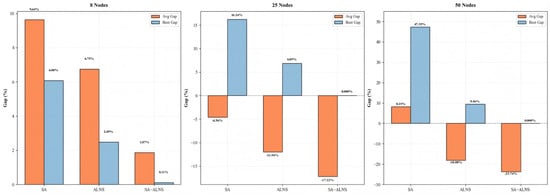
Figure 4. Performance of algorithms across different sizes.

The robustness advantage of S-ALNS becomes even more evident on large-scale benchmark instances, as summarized in Table 10. Across all tested datasets, S-ALNS consistently outperforms standard ALNS. For the KroA100 instance, S-ALNS achieves best and average gaps of −18.70% and −15.99%, compared with −17.45% and −14.48% obtained by ALNS. This performance difference increases with problem scale. On KroA200, the average gap is improved from −18.10% to −20.38%, while on Rd400, it improves from −1.11% to −2.58%. It is worth noting that both S-ALNS and ALNS identify the same optimal fleet sizes—2, 3, and 4 vehicles for KroA100, KroA200, and Rd400, respectively—indicating consistent convergence behavior with respect to fleet configuration decisions.

In terms of computational efficiency, S-ALNS incurs slightly higher runtimes than SA and ALNS for small-scale instances (approximately 5.00–5.24 s versus sub-second execution times). However, as illustrated in Figure 5, this difference becomes less pronounced as the problem scale increases. The moderate increase in computational effort is compensated by substantial improvements in solution quality, indicating a favorable trade-off between efficiency and performance.

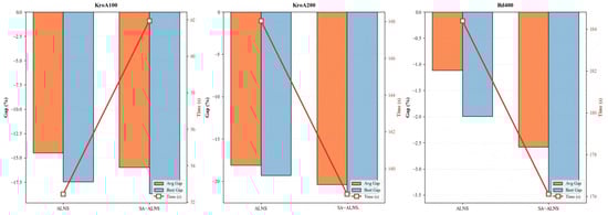
Figure 5. Performance of algorithms across large sizes.

Overall, the robustness analysis demonstrates that S-ALNS consistently delivers high-quality solutions across a wide range of problem scales while maintaining practical computational efficiency. Its ability to achieve near-zero optimality gaps on medium-scale instances and to significantly outperform baseline methods on large-scale benchmarks highlights its reliability and suitability for real-world VRPD applications.

5.4. Managerial Insights

Beyond numerical performance comparisons, the experimental results provide several insights that are particularly relevant for logistics decision-makers. The insights are structured along two dimensions. The first evaluates the system-level benefits of introducing drones by comparing truck-only and truck-drone collaborative operations. The second examines the role of drone operating time in achieving efficiency gains without increasing planning complexity.

Impact of drone participation. The experimental results provide clear managerial evidence that integrating drones into truck-based delivery systems can generate substantial system-level benefits, even when each truck is equipped with at most one drone. By allowing multiple trucks to operate concurrently, each coordinating with its assigned drone, the overall routing system gains significant flexibility in task allocation and spatial coverage. Across all tested instances (see Figure 6), drone participation consistently leads to pronounced reductions in total operational cost under identical spatial configurations. These improvements stem from the drones’ ability to selectively serve spatially inefficient customers, thereby shortening truck routes, reducing detours, and mitigating time-window penalties. Importantly, the benefits are particularly pronounced in instances with dispersed or clustered customer distributions, where traditional truck-only routing tends to incur high marginal costs.

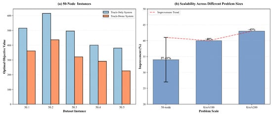
Figure 6. Performance improvement in a truck-drone collaborative system.

From a managerial perspective, the results indicate that the value of drones lies not in replacing trucks, but in complementing them as mobile launch-and-recovery assets within a coordinated fleet. Such a deployment strategy enables logistics operators to achieve large performance gains without increasing fleet size or computational burden. Moreover, the stable runtime observed across all instances suggests that these improvements are achievable without sacrificing planning efficiency, making truck-drone collaboration a practical and scalable option for real-world logistics operations.

Impact of drone operating time. Figure 7 reports the system-level delivery time under different maximum drone flight time limits, assuming a fixed drone payload capacity of 20 kg. Across all datasets, extending the allowable drone operating time consistently reduces the overall delivery time, confirming that drone endurance is a critical lever for improving system efficiency.

Figure 7. Impact of drone flight duration on total delivery time.

The most significant performance gains occur when the maximum flight time increases from 20 to 40 min. On average, this extension reduces the total delivery time by approximately 20–25%, as it enables drones to serve a larger set of customers directly and to operate over longer truck-drone separation distances. This observation suggests that short-range drones may severely limit the potential benefits of truck-drone collaboration. Beyond 60 min, however, the marginal improvement becomes noticeably smaller. Extending the flight time from 60 to 80 min yields only modest or, in some cases, negligible reductions in delivery time. This diminishing-return pattern indicates that excessively long drone endurance does not proportionally translate into additional system-level benefits once most feasible drone tasks have already been covered.

From a managerial perspective, these results highlight an important trade-off. Investing in moderate drone endurance (approximately 40–60 min) captures the majority of operational benefits, whereas further extending flight time may lead to limited efficiency gains relative to the associated increases in acquisition cost, energy consumption, and maintenance complexity.

6. Conclusions

This paper investigates drone-assisted last-mile delivery, with an emphasis on optimizing collaborative routing between trucks and drones to improve delivery efficiency and reduce overall completion time. We propose a novel multi-truck, multi-drone routing model in which both vehicles are allowed to perform multiple trips under capacity constraints, thereby overcoming the limitations of traditional single-visit delivery schemes. The proposed formulation effectively captures the operational complexity of large-scale parcel distribution systems and provides a flexible framework for coordinated truck-drone operations.

To address the resulting NP-hard VRPD, we develop a three-phase Structure-Guided Adaptive Large Neighborhood Search (S-ALNS) algorithm. The proposed solution framework consists of (i) an efficient initial truck route construction phase based on clustering and load-balanced assignment, (ii) a drone assignment phase employing an enhanced split heuristic to identify customers suitable for aerial delivery, and (iii) a refinement phase built upon an improved ALNS framework with advanced destroy and repair operators. In particular, the incorporation of dynamic programming within the repair phase enables efficient batch insertion decisions, leading to substantial improvements in solution quality while maintaining manageable computational complexity across different problem scales.

Extensive computational experiments demonstrate the effectiveness and scalability of the proposed S-ALNS algorithm. For small-scale instances, S-ALNS consistently generates near-optimal solutions with very small optimality gaps. For medium-scale instances, it outperforms the best feasible solutions obtained by the Gurobi solver within practical time limits. For large-scale benchmark instances, S-ALNS preserves strong solution quality while remaining computationally efficient, consistently outperforming benchmark metaheuristics. Overall, the algorithm achieves optimality gaps as low as 0.108% on small instances and exhibits robust performance across all tested problem scales.

In conclusion, the proposed model and solution framework highlight the significant advantages of multi-visit, multi-truck, and multi-drone collaboration in modern last-mile logistics. The strong and stable performance of S-ALNS across diverse instance sizes suggests its practical applicability to real-world delivery systems. Future research will extend the proposed framework to dynamic and stochastic settings, incorporating real-time delivery requests, traffic-dependent travel times, and adaptive collaboration strategies. Further investigation into the interactions among delivery demand distributions, spatial customer patterns, and truck-drone coordination mechanisms also represents a promising direction for improving system-level efficiency.

References

- Newcomb, A. Alibaba Beats Amazon to Drone Delivery. ABC News. 2015. Available online: https://abcnews.go.com/Technology/alibaba-beats-amazon-drone-delivery/story?id=28720942 (accessed on 17 August 2023).
- Murphy, M. This Is How Google Wants Its Drones to Deliver Stuff to You. Quartz. 2016. Available online: https://qz.com/670670/this-is-how-google-wants-its-drones-to-deliver-stuff-to-you/ (accessed on 17 August 2023).
- Kee, E. DHL’s Failed Drone Demonstration. Ubergizmo. 2016. Available online: https://www.ubergizmo.com/2016/01/dhls-failed-drone-demonstration/ (accessed on 17 August 2023).
- Holland, C.; Levis, J.; Nuggehalli, R.; Santilli, B.; Winters, J. UPS optimizes delivery routes. Interfaces 2017, 47, 8–23. [Google Scholar] [CrossRef]
- Cui, R.; Li, M.; Li, Q. Value of high-quality logistics: Evidence from a clash between SF Express and Alibaba. Manag. Sci. 2020, 66, 3879–3902. [Google Scholar] [CrossRef]
- Kunovjanek, M.; Wankmüller, C. Containing the COVID-19 pandemic with drones—Feasibility of a drone enabled back-up transport system. Transp. Policy 2021, 106, 141–152. [Google Scholar] [CrossRef] [PubMed]
- Wohlsen, M. The Next Big Thing You Missed: Amazon’s Delivery Drones Could Work—They Just Need Trucks. Wired.com. 2014. Available online: http://www.wired.com/2014/06/the-next-big-thing-you-missed-delivery-drones-launched-from-trucks-are-the-future-of-shipping/ (accessed on 17 August 2023).
- Murray, C.C.; Chu, A.G. The flying sidekick traveling salesman problem: Optimization of drone-assisted parcel delivery. Transp. Res. Part C Emerg. Technol. 2015, 54, 86–109. [Google Scholar] [CrossRef]
- Poikonen, S.; Wang, X.; Golden, B. The vehicle routing problem with drones: Extended models and connections. Networks 2017, 70, 34–43. [Google Scholar] [CrossRef]
- Wang, X.; Poikonen, S.; Golden, B. The vehicle routing problem with drones: Several worst-case results. Optim. Lett. 2017, 11, 679–697. [Google Scholar] [CrossRef]
- Zhou, H.; Qin, H.; Cheng, C.; Rousseau, L.-M. An exact algorithm for the two-echelon vehicle routing problem with drones. Transp. Res. Part B Methodol. 2023, 168, 124–150. [Google Scholar] [CrossRef]
- Tamke, F.; Buscher, U. A branch-and-cut algorithm for the vehicle routing problem with drones. Transp. Res. Part B Methodol. 2021, 144, 174–203. [Google Scholar] [CrossRef]
- Bouman, P.; Agatz, N.; Schmidt, M. Dynamic programming approaches for the traveling salesman problem with drone. Networks 2018, 72, 528–542. [Google Scholar] [CrossRef]
- Schermer, D.; Moeini, M.; Wendt, O. A hybrid VNS/Tabu search algorithm for solving the vehicle routing problem with drones and en route operations. Comput. Oper. Res. 2019, 109, 134–158. [Google Scholar] [CrossRef]
- Salama, M.R.; Srinivas, S. Collaborative truck multi-drone routing and scheduling problem: Package delivery with flexible launch and recovery sites. Transp. Res. Part E Logist. Transp. Rev. 2022, 164, 102788. [Google Scholar] [CrossRef]
- Sacramento, D.; Pisinger, D.; Ropke, S. An adaptive large neighborhood search metaheuristic for the vehicle routing problem with drones. Transp. Res. Part C Emerg. Technol. 2019, 102, 289–315. [Google Scholar] [CrossRef]
- Braekers, K.; Ramaekers, K.; Van Nieuwenhuyse, I. The vehicle routing problem: State of the art classification and review. Comput. Ind. Eng. 2016, 99, 300–313. [Google Scholar] [CrossRef]
- Zhen, L.; Gao, J.; Tan, Z.; Wang, S.; Baldacci, R. Branch-price-and-cut for trucks and drones cooperative delivery. IISE Trans. 2023, 55, 271–287. [Google Scholar] [CrossRef]
- Kitjacharoenchai, P.; Ventresca, M.; Moshref-Javadi, M.; Lee, S.; Tanchoco, J.M.A.; Brunese, P.A. Multiple traveling salesman problem with drones: Mathematical model and heuristic approach. Comput. Ind. Eng. 2019, 129, 14–30. [Google Scholar] [CrossRef]
- Wang, Z.; Sheu, J.-B. Vehicle routing problem with drones. Transp. Res. Part B Methodol. 2019, 122, 350–364. [Google Scholar] [CrossRef]
- Liu, Y.; Liu, Z.; Shi, J.; Wu, G.; Pedrycz, W. Two-echelon routing problem for parcel delivery by cooperated truck and drone. IEEE Trans. Syst. Man Cybern. Syst. 2020, 51, 7450–7465. [Google Scholar] [CrossRef]
- Lemardelé, C.; Estrada, M.; Pagès, L.; Bachofner, M. Potentialities of drones and ground autonomous delivery devices for last-mile logistics. Transp. Res. Part E Logist. Transp. Rev. 2021, 149, 102325. [Google Scholar] [CrossRef]
- Schermer, D.; Moeini, M.; Wendt, O. A matheuristic for the vehicle routing problem with drones and its variants. Transp. Res. Part C Emerg. Technol. 2019, 106, 166–204. [Google Scholar] [CrossRef]
- Kitjacharoenchai, P.; Min, B.-C.; Lee, S. Two echelon vehicle routing problem with drones in last mile delivery. Int. J. Prod. Econ. 2020, 225, 107598. [Google Scholar] [CrossRef]
- Wang, K.; Pesch, E.; Kress, D.; Fridman, I.; Boysen, N. The Piggyback Transportation Problem: Transporting drones launched from a flying warehouse. Eur. J. Oper. Res. 2022, 296, 504–519. [Google Scholar] [CrossRef]
- Poikonen, S.; Golden, B. Multi-visit drone routing problem. Comput. Oper. Res. 2020, 113, 104802. [Google Scholar] [CrossRef]
- Euchi, J.; Sadok, A. Hybrid genetic-sweep algorithm to solve the vehicle routing problem with drones. Phys. Commun. 2021, 44, 101236. [Google Scholar] [CrossRef]
- Roberti, R.; Ruthmair, M. Exact methods for the traveling salesman problem with drone. Transp. Sci. 2021, 55, 315–335. [Google Scholar] [CrossRef]
- Gonzalez-R, P.L.; Canca, D.; Andrade-Pineda, J.L.; Calle, M.; Leon-Blanco, J.M. Truck-drone team logistics: A heuristic approach to multi-drop route planning. Transp. Res. Part C Emerg. Technol. 2020, 114, 657–680. [Google Scholar] [CrossRef]
- Gao, J.; Zhen, L.; Wang, S. Multi-trucks-and-drones cooperative pickup and delivery problem. Transp. Res. Part C Emerg. Technol. 2023, 157, 104407. [Google Scholar] [CrossRef]
- Mara, S.T.W.; Norcahyo, R.; Jodiawan, P.; Lusiantoro, L.; Rifai, A.P. A survey of adaptive large neighborhood search algorithms and applications. Comput. Oper. Res. 2022, 146, 105903. [Google Scholar] [CrossRef]
- Voigt, S. A review and ranking of operators in adaptive large neighborhood search for vehicle routing problems. Eur. J. Oper. Res. 2025, 322, 357–375. [Google Scholar] [CrossRef]
- Karakostas, P.; Sifaleras, A. A double-adaptive general variable neighborhood search algorithm for the solution of the traveling salesman problem. Appl. Soft Comput. 2022, 121, 108746. [Google Scholar] [CrossRef]
- Karakostas, P.; Sifaleras, A. Learning-assisted improvements in Adaptive Variable Neighborhood Search. Swarm Evol. Comput. 2025, 94, 101887. [Google Scholar] [CrossRef]
- Agatz, N.; Bouman, P.; Schmidt, M. Optimization approaches for the traveling salesman problem with drone. Transp. Sci. 2018, 52, 965–981. [Google Scholar] [CrossRef]
- Ha, Q.M.; Deville, Y.; Pham, Q.D.; Hà, M.H. On the min-cost traveling salesman problem with drone. Transp. Res. Part C Emerg. Technol. 2018, 86, 597–621. [Google Scholar] [CrossRef]
- Luo, Z.; Poon, M.; Zhang, Z.; Liu, Z.; Lim, A. The multi-visit traveling salesman problem with multi-drones. Transp. Res. Part C Emerg. Technol. 2021, 128, 103172. [Google Scholar] [CrossRef]
- Ropke, S.; Pisinger, D. A unified heuristic for a large class of vehicle routing problems with backhauls. Eur. J. Oper. Res. 2006, 171, 750–775. [Google Scholar] [CrossRef]
- Luo, Z.; Gu, R.; Poon, M.; Liu, Z.; Lim, A. A last-mile drone-assisted one-to-one pickup and delivery problem with multi-visit drone trips. Comput. Oper. Res. 2022, 148, 106015. [Google Scholar] [CrossRef]
- Ropke, S.; Pisinger, D. An adaptive large neighborhood search heuristic for the pickup and delivery problem with time windows. Transp. Sci. 2006, 40, 455–472. [Google Scholar] [CrossRef]
Disclaimer/Publisher’s Note: The statements, opinions and data contained in all publications are solely those of the individual author(s) and contributor(s) and not of MDPI and/or the editor(s). MDPI and/or the editor(s) disclaim responsibility for any injury to people or property resulting from any ideas, methods, instructions or products referred to in the content. |
© 2026 by the authors. Licensee MDPI, Basel, Switzerland. This article is an open access article distributed under the terms and conditions of the Creative Commons Attribution (CC BY) license.