Machine Learning and Operator-Based Nonlinear Internal Model Control Design for Soft Robotic Finger Using Robust Right Coprime Factorization

Abstract

Currently, machine learning (ML) methods provide a practical approach to model complex systems. Unlike purely analytical models, ML methods can describe the uncertainties (e.g., hysteresis, temperature effects) that are difficult to deal with, potentially yielding higher-precision dynamics by a learning plant given a high-volume dataset. However, employing learning plants that lack explicit mathematical representations in real-time control remains challenging, namely, the model can be conversely looked at as a mapping from input data to output, and it is difficult to represent the corresponding time relationships in real applications. Hence, an ML and operator-based nonlinear control design is proposed in this paper. In this new framework, the bounded input/output spaces of the learning plant are addressed rather than mathematical dynamic formulation, which is realized by robust right coprime factorization (RRCF). While the stabilized learning plant is explored by RRCF, the desired tracking performance is also considered by an operator-based nonlinear internal model control (IMC) design. Eventually, practical application on a soft robotic finger system is conducted, which indicates the better performance of using the controlled learning plant and the feasibility of the proposed framework.

1. Introduction

In recent years, machine learning (ML) methods have attracted considerable interest from researchers, and have been widely applied in various fields like computer vision [1,2,3,4], system identification [5,6,7], robotics [8,9,10,11,12], and so on. Specifically, driven by large-scale datasets, ML offers new approaches to describe the dynamics of complex industrial systems whose analytical mathematical models are difficult to compute [13]. Given the obtained learning plant (i.e., the trained ML model), several frameworks were introduced to address the control issue. For example, a neural network (NN)-based nonlinear internal model control (IMC) structure was constructed in [14], where neural networks were selected to design the inverse model of IMC; a similar NN-based IMC structure can also be found in [15], which motivates further exploration of ML-IMC combinations; besides IMC, NN predictive control was proposed in [16], which dealt with the delay issue using recurrent NNs for nonlinear plants; an adaptive control framework was depicted in [17], where the NN played roles in both online identification and parameters adjustment; and for a multi-mode process, an LSTM-based model predictive control scheme was depicted in [18], which automatically matched different operation modes without switching strategies. However, the aforementioned studies rely on the dynamics of ML methods or objective systems, which makes the analysis of stability or tracking performance complicated. In addition, for those ML methods or systems whose dynamics are not concisely modeled, one may find it difficult to apply such control designs.

As one of the well-established nonlinear control strategies, the operator theory is implemented in this work. According to operator theory, a given nonlinear plant can be interpreted as an operator that maps from its input space towards its output space. In contrast to control schemes whose design depends on accurate system dynamics, a robust right coprime factorization (RRCF) feedback structure is established given the input/output spaces of each operator. Hence, RRCF realizes nonlinear control from the perspective of operators, namely, input–output mappings. RRCF has been practically applied in Hamiltonian systems [19], micro-hand actuator system [20], etc [21,22]. Moreover, RRCF was combined with ML methods like multi support vector regression for soft actuators in [23] and with a neural network to address the denial of service attacks in [24], where the learning plant is reliable in real applications. For learning plants that lack an explicit mathematical model and time relationships, their input–output mappings coincide with the characteristics of RRCF, which makes RRCF a potential approach to stabilize learning plants.

Motivated by the aforementioned issues, the main contributions of this work are outlined as follows:

• An operator-based control design for machine learning models is established in the RRCF feedback structure, which ensures the robust stability of machine learning models by input–output mappings rather than explicit mathematical dynamics. Such compensation by RRCF for machine learning models provides security for practical implementation.
• The proposed RRCF feedback system for machine learning models is inserted into a nonlinear IMC framework. Such a combination contributes to the finite tracking convergence of output, even with potential jumps or perturbation.
• As a practical application of the proposed control design, experiments with a soft robotic finger are conducted. The comparative results indicate the feasibility and superiority of this framework.

The remainder of this paper is organized as follows. Section 2 introduces the mathematical preliminaries of RRCF. Section 3 describes the proposed control design, which includes the stabilization of the learning plant and analysis of tracking performance. Section 4 exhibits the practical experiments with the soft robotic finger. The whole work is concluded in Section 5.

2. Preliminaries

In this section, some mathematical preliminaries on nonlinear robust right coprime factorization (RRCF) will be briefly introduced. Initially, nonlinear right factorization is described as follows.

Consider the objective target plant, which is denoted by $\mathit{P}$. $\mathit{P}$ is of nonlinear dynamics, and is analyzed from the perspective of an operator, i.e., $\mathit{P}$ is a mapping from $\mathit{U}$ to $\mathit{Y}$, which are the input space and output space, respectively. It should be noted that in the real world, such spaces are defined as associated with Banach space in the time domain. Assume two bounded subspaces in $\mathit{U}$ and $\mathit{Y}$ as ${\mathit{u}}_s$ and ${\mathit{Y}}_s$, then $\mathit{P}$ is said to be stable if $\mathit{P}\left(U_s\right)\subseteq Y_s$. In other words, a stable operator maps bounded input space into bounded output space. However, $\mathit{P}$ is potentially unstable, while indicating unbounded output space. To stabilize $\mathit{P}$, one first defines the right factorization of $\mathit{P}$ as

$$P=N{D}^{-1}$$

(1)

where $\mathit{P}$ is factorized into two individual operators, analytically. The internal variable is defined as a quasi-state of $\mathit{P}$, denoted by $\omega \left(t\right)\in W_s$ and ${\mathit{W}}_s$ is a subspace of $\mathit{W}$. Then, one can write $\omega \left(t\right)=D^{-1}\left(u\right)\left(t\right)$, $\mathit{y}\left(t\right)=N\left(\omega \right)\left(t\right)$. Here the requirements of $\mathit{N}$ and ${\mathit{D}}^{-1}$ are listed as follows:

• $\mathit{N}$ is stable from ${\mathit{W}}_s$ to ${\mathit{Y}}_s$.
• ${\mathit{D}}^{-1}$ is potentially unstable (inherits from $\mathit{P}$). However, ${\mathit{D}}^{-1}$ is invertible between $\mathit{W}$ and $\mathit{U}$, while $\mathit{D}$ is stable from ${\mathit{W}}_s$ to ${\mathit{U}}_s$.

Next, given the right factorization of $\mathit{P}$, a feedback system is constructed, which is depicted as Figure 1. To realize the stabilization of $\mathit{P}$, one needs other controllers $\mathit{S}$ and $\mathit{R}$, by which the following Bezout Identity [19]

$$SN+RD=M_1$$

(2)

is satisfied. The designed $\mathit{S}$, $\mathit{R}$, and $\mathit{M}$ are described as follows:

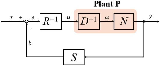
Figure 1. General scheme of right coprime factorization (RCF).

• $\mathit{R}$ maps ${\mathit{U}}_s$ to ${\mathit{U}}_s$, i.e., $\mathit{e}\left(t\right)\in U_s$, $\mathit{e}\left(t\right)=R\left(u\right)\left(t\right)$. $\mathit{R}$ is stable and invertible. ${\mathit{R}}^{-1}$ is stable.
• $\mathit{S}$ maps ${\mathit{Y}}_s$ to ${\mathit{U}}_s$, i.e., $\mathit{b}\left(t\right)\in U_s$, $\mathit{b}\left(t\right)=S\left(y\right)\left(t\right)$. $\mathit{S}$ is stable.
• ${\mathit{M}}_1$ maps ${\mathit{W}}_s$ to ${\mathit{U}}_s$, i.e., $\mathit{r}\left(t\right)=M_1\left(\omega \right)\left(t\right)$. ${\mathit{M}}_1$ is stable and invertible, ${\mathit{M}}_1^{-1}$ is stable. An operator like ${\mathit{M}}_1$ is defined as a unimodular operator (both ${\mathit{M}}_1$ and ${\mathit{M}}_1^{-1}$ are stable).

Given the Bezout Identity, one can find that each of the variables $\mathit{e}$, $\mathit{u}$, $\omega$, $\mathit{y}$, and $\mathit{b}$ are stable (bounded) if the reference input $\mathit{r}$ is bounded. Hence, it is called bounded input bounded output (BIBO) stable.

More generally, consider the potential uncertainty in a real-world scenario; RRCF is discussed to explore the robustness of such a feedback scheme. In Figure 2, $\Delta P$ denotes the bounded uncertainty and is factorized into $\Delta N$ as $(P+\Delta P)=(N+\Delta N)D^{-1}$. Then, one can rewrite the Bezout Identity as

$$S(N+\Delta N)+RD=M_2$$

(3)

where ${\mathit{M}}_2$ can be found to be unimodular if $\mathit{S}$ and $\Delta N$ satisfy the following inequality [19]

$$\parallel (S(N+\Delta N)-SN)M_1^{-1}\parallel <1$$

(4)

where $\parallel ·\parallel$ is the Lipschitz semi-norm, which is defined as

$$\parallel Q\parallel =\underset{T\in [0,\infty )}{sup}\underset{\begin{array}{c}u,\tilde{u}\in U_s\\ u_T\ne {\tilde{u}}_T\end{array}}{sup}{\displaystyle \frac{{|\left[Q\left(u\right)\right]}_T-{\left[Q\left(\tilde{u}\right)\right]}_T{|}_{Y_B}}{|u_T-{\tilde{u}}_T{|}_{U_B}}}$$

(5)

for an nominal operator $\mathit{Q}\left(U_s\right)\subseteq Y_s$, and ${\mathit{U}}_B$, ${\mathit{Y}}_B$ denote the associated Banach spaces, respectively.

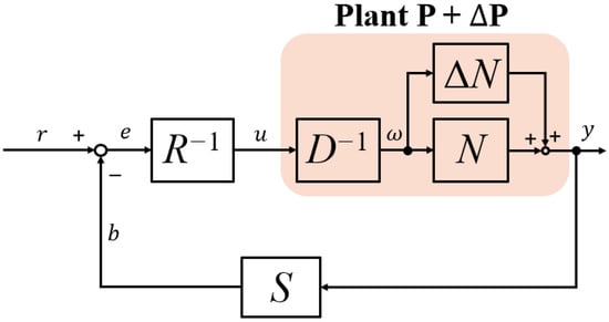
Figure 2. General scheme of robust right coprime factorization (RRCF).

3. Main Results

In this section, the basic scheme of a machine learning-based nonlinear internal control design will be described. The proposed scheme is established following the operator control theory and in the form of right coprime factorization. Moreover, the stability analysis and tracking performance of the system will be presented.

3.1. Problem Statement

Initially, the problem addressed in this paper is described here, which starts from the notations of the objective nonlinear plant, i.e.,

$$\begin{array}{cc}\hfill y_0\left(t\right)& =P_{nominal}\left(u\right)\left(t\right)=P_0\left(u\right)\left(t\right)\hfill \end{array}$$

(6)

$$\begin{array}{cc}\hfill \widehat{y}\left(t\right)& =P_{learning}\left(u\right)\left(t\right)=(P_0+\Delta P_0+d_0)\left(u\right)\left(t\right)\hfill \end{array}$$

(7)

$$\begin{array}{cc}\hfill y\left(t\right)& =P_{real}\left(u\right)\left(t\right)=(P_0+\Delta P+d)\left(u\right)\left(t\right)\hfill \end{array}$$

(8)

where ${\mathit{P}}_{nominal}$ denotes the mathematical dynamics (also noted as ${\mathit{P}}_0$) of the objective plant, which is generally derived from physical analysis; ${\mathit{P}}_{learning}$ serves as the model obtained by machine learning, such as support vector regression and neural network; and ${\mathit{P}}_{real}$ is the physical plant in the real world, i.e., the target system. ${\mathit{y}}_0$, $\widehat{y}$, and $\mathit{y}$ denote the outputs in different scenarios, respectively, and $\mathit{u}$ is the input. $\Delta P$ represents the uncertainty that is difficult to analytically model or compute, which is approximated by the collected dataset and modeled as $\Delta P_0$ using machine learning. ${\mathit{d}}_0$ represents the measurement perturbation that naturally occurs during data collection. $\mathit{d}$ denotes the perturbation in real-world operation, as well as the mismatch between the learning plant and real-world dynamics. To describe the plant as an operator, all variables are defined in the time domain. Although $\mathit{d}$ may contain a component similar to ${\mathit{d}}_0$, there are assumed to be no probabilistic relations between $\mathit{d}$ and ${\mathit{d}}_0$.

The problems addressed in this paper can be summarized as follows:

• In many cases, uncertainties and perturbation cannot be precisely captured, which results in a significant discrepancy between nominal models and real plants. This may affect performance (e.g., tracking accuracy). Hence, the usage of well-trained machine-learning models for control design needs to be investigated.
• Despite their accurate approximation of real plants, learning models often do not admit a mathematical formulation and are commonly characterized as input–output relations. Therefore, ensuring closed-loop stability and satisfactory performance requires careful consideration in the control design.

3.2. Scheme of the Proposed Control Design

To address the aforementioned problems, the proposed control design can be depicted as in Figure 3, which is composed of an operator-based nonlinear internal model mechanism [25] and tracking compensation. “ML plant” and “Real plant” stand for machine learning model ${\mathit{P}}_{learning}$ and real plant ${\mathit{P}}_{real}$, respectively. Next, the specific details of each operator and controller will be described.

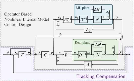
Figure 3. The proposed nonlinear internal model control design.

Given the definitions (6)–(8), the right factorization of different plants can be formulated as

$$\begin{array}{cc}\hfill y_0\left(t\right)& =P_0\left(u\right)\left(t\right)=N{D}^{-1}\left(u\right)\left(t\right)\hfill \end{array}$$

(9)

$$\begin{array}{cc}\hfill \widehat{y}\left(t\right)& =(P_0+\Delta P_0+d_0)\left(u\right)\left(t\right)=(N+\Delta N_0+d_0)D^{-1}\left(u\right)\left(t\right)\hfill \end{array}$$

(10)

$$\begin{array}{cc}\hfill y\left(t\right)& =(P_0+\Delta P+d)\left(u\right)\left(t\right)=(N+\Delta N+d)D^{-1}\left(u\right)\left(t\right)\hfill \end{array}$$

(11)

where ${\mathit{D}}^{-1}$ denotes the potentially unstable component, and the uncertainty ($\Delta N_0$, $\Delta N$) and perturbation ($\mathit{d}$, ${\mathit{d}}_0$) that exist with $\mathit{N}$ are represented. Further, the following discussion is limited to the representation of the ML plant (10). Here one can find the bounded stability of $N+\Delta N_0+d_0$ and $N+\Delta N+d$ given the assumption of boundedness: $\parallel \Delta N_0{(·)\parallel }_{\infty }\le \Delta {\overline{N}}_0$, ${\parallel \Delta N(·)\parallel }_{\infty }\le \Delta \overline{N}$, $\parallel d_0{(·)\parallel }_{\infty }\le \overline{d_0}$, ${\parallel d(·)\parallel }_{\infty }\le \overline{d}$.

In this work, the operators $\mathit{A}$ and $\mathit{B}$ are designed with a nominal plant. That is, by designing the proper $\mathit{A}$ and $\mathit{B}$, one has to satisfy the Bezout Identity (2), which ensures the robust stability of the real plant by the unimodular operator $\mathit{M}$, though the “perturbed” Bezout Identity is likely to be unknown. Moreover, for the feedback loop of the ML plant, ${\mathit{A}}_0$ and ${\mathit{B}}_0$ offer much more freedom according to the input/output space of the ML plant, which is already known as dataset. However, such a design of ${\mathit{A}}_0$ and ${\mathit{B}}_0$ remains constrained by the Bezout Identity (2). This is aimed at the stabilization of the learning plant ${\mathit{P}}_{learning}$, since the input/output variation is required to be within its corresponding stable space, though some perturbation or finite jumps potentially exist in the sequence. In other words, owing to the robustness and “bounded space mapping” perspective of the RRCF feedback system, the stability analysis no longer requires a precise model of the perturbation or uncertainties. In the following analysis, to validate the feasibility of the proposed design, for simplicity, ${\mathit{A}}_0$ and ${\mathit{B}}_0$ are assumed to be designed to have the same structure as $\mathit{A}$ and $\mathit{B}$ in this paper, i.e., ${\mathit{A}}_{0}N+B_{0}D=AN+BD=M$, leaving possibly different designs for future works. As a result, a compensated learning plant is realized by the RRCF feedback loop according to Figure 3.

Next, following the description of designed operators $\mathit{A},B,A_0$, and ${\mathit{B}}_0$, the proposed control design will first be analyzed without considering tracking compensation, i.e., $\tilde{e}\left(t\right)=\overline{r}\left(t\right)-\tilde{y}\left(t\right)$. According to the principle of an internal model control mechanism, a stable controller $\mathit{C}$ will be designed to satisfy

$$N{M}^{-1}C(·)=I(·)$$

(12)

where $\mathit{I}$ is an Identity operator and bounded. However, one will find that given the existence of uncertainty and perturbation in the ML plant, the Bezout Identity has to be rewritten as

$$A_0(N+\Delta N_0+d_0)+B_{0}D=\tilde{M}$$

(13)

where $\tilde{M}$ remains unimodular if satisfying the condition (4) on the robust stability of right coprime factorization. Then, $\widehat{y}$ can be formulated as

$$\widehat{y}\left(t\right)=(N+\Delta N_0+d_0){\tilde{M}}^{-1}C\left(\tilde{e}\right)\left(t\right)$$

(14)

which results in

$$\widehat{y}\left(t\right)-\tilde{e}\left(t\right)=[(N+\Delta N_0+d_0){\tilde{M}}^{-1}C-I]\left(\tilde{e}\right)\left(t\right)$$

(15)

provided that $(N+\Delta N_0+d_0)$, ${\tilde{M}}^{-1}$ and $\mathit{C}$ are bounded, one can write (15) as

$$\widehat{y}\left(t\right)=\tilde{e}\left(t\right)+ϵ\left(t\right)$$

(16)

where ${\parallel ϵ\left(t\right)\parallel }_{\infty }\le \overline{ϵ}$ for any bounded $\tilde{e}\left(t\right)$. Hence, according to the nonlinear internal model control mechanism, $\tilde{e}\left(t\right)=\overline{r}\left(t\right)-\tilde{y}\left(t\right)$, $\tilde{y}\left(t\right)=y\left(t\right)-\widehat{y}\left(t\right)$, then

$$\overline{r}\left(t\right)-y\left(t\right)=-ϵ\left(t\right)$$

(17)

which indicates the convergence of output of the real plant in a ball of $\overline{r}$ with its radius of $\overline{ϵ}$. Although the replacement of the “ML plant” with the nominal plant introduces a deviation within the ball, it can practically be compensated by the tracking controller and hence has a trivial influence on the system. In contrast, in particular, the relatively smaller difference $\tilde{y}$ reduces the risk of output saturation, ensuring that the system is within the robust stable region. This analysis will be validated by the experiments in the next section.

Besides the internal model control design, another controller $\mathit{F}$ is selected to guarantee the tracking compensation. Specifically, $\mathit{F}$ is formulated as a Proportional–Integral controller:

$$\begin{array}{cc}\hfill x_e\left(t\right)& =\tilde{r}\left(t\right)-y\left(t\right)\hfill \end{array}$$

(18)

$$\begin{array}{cc}\hfill F\left(x_e\right)\left(t\right)& =K_P{x}_e\left(t\right)+K_I{\int }_0^t{x}_e\left(\tau \right)d\tau \hfill \end{array}$$

(19)

then (17) can be rewritten as

$$\begin{array}{cc}\hfill \tilde{r}\left(t\right)-y\left(t\right)& =-F\left(x_e\right)\left(t\right)-ϵ\left(t\right)\hfill \\ \hfill & =-x_e\left(t\right)\hfill \end{array}$$

(20)

by which the dynamics of ${\mathit{x}}_e\left(t\right)$ can be derived as

$${\dot{x}}_e\left(t\right)=-\alpha x_e\left(t\right)-\beta \dot{ϵ}\left(t\right)$$

(21)

where

$$\alpha ={\displaystyle \frac{K_I}{K_P+1}},\beta ={\displaystyle \frac{1}{K_P+1}}$$

(22)

by selecting ${\mathit{K}}_P>-1$ and ${\mathit{K}}_I>0$, one can find $\alpha >0$ and $\beta >0$. However, with the presence of finite jumps or perturbation, $\dot{ϵ}$ in the right hand is likely to be too large and even unbounded in certain moments, which makes it difficult for stability analysis. In this work, inspired by the results of impulsive differential equations introduced in [26], the dynamics (21) are analyzed both in flow and jump intervals by defining

$$z\left(t\right):=x_e\left(t\right)+\beta ϵ\left(t\right)$$

(23)

If $ϵ\left(t\right)$ has a jump $\Delta ϵ\left(t_k\right):=ϵ\left(t_k^{+}\right)-ϵ\left(t_k^{-}\right)$ at $t_k$, $\mathit{k}=1,2,\dots$, then integrate (21) over $(t_k-\eta ,t_k+\eta )$ and let $\eta \to 0$:

$$\begin{array}{cc}\hfill & \int {\dot{x}}_{e}dt+\alpha \int x_{e}dt+\beta \int dϵ\hfill \\ \hfill =& \Delta x_e\left(t_k\right)+\alpha \int x_{e}dt+\beta \Delta ϵ\left(t_k\right)\hfill \\ \hfill =& 0,\hfill \end{array}$$

(24)

and the middle integral vanishes as the interval shrinks, which results in

$$\Delta x_e\left(t_k\right):=x_e\left(t_k^{+}\right)-x_e\left(t_k^{-}\right)=-\beta \Delta ϵ\left(t_k\right)$$

(25)

Introducing (25) into the derivation of (23), one can find $\Delta z\left(t_k\right)=\Delta x_e\left(t_k\right)+\beta \Delta ϵ\left(t_k\right)=0$, which indicates that z is continuous at jumps. During flow intervals (between jumps),

$$\dot{z}\left(t\right)={\dot{x}}_e\left(t\right)+\beta \dot{ϵ}\left(t\right)=-\alpha x_e\left(t\right)=-\alpha (z\left(t\right)-\beta ϵ\left(t\right))$$

(26)

for any $t\ge t_0$, this leads to

$$z\left(t\right)=e^{-\alpha (t-t_0)}z\left(t_0\right)+\alpha \beta {\int }_{t_0}^t{e}^{-\alpha (t-s)}ϵ\left(s\right)ds$$

(27)

consequently, the convergence of $\mathit{z}\left(t\right)$ is obtained as

$$\left|z\left(t\right)\right|\le e^{-\alpha (t-t_0)}\left|z\left(t_0\right)\right|+\beta \left(1-e^{-\alpha (t-t_0)}\right)\overline{ϵ}$$

(28)

and since $x=z-\beta \epsilon$, one can write the limits as

$$\begin{array}{cc}\hfill & \underset{t\to \infty }{\text{lim sup}}\left|z\left(t\right)\right|\le \beta \overline{ϵ}\hfill \\ \hfill & \underset{t\to \infty }{\text{lim sup}}\left|x_e\left(t\right)\right|\le 2\beta \overline{ϵ}\hfill \end{array}$$

(29)

Hence, by tuning ${\mathit{K}}_{\mathit{P}}$, ${\mathit{K}}_I$, the tracking error ${\mathit{x}}_{\mathit{e}}\left(t\right)$ will be uniformly ultimately bounded within trivial $\overline{ϵ}$; moreover, in particular, if $ϵ\left(t\right)$ settles as a constant, i.e., $ϵ\left(t\right)\to {ϵ}_{\infty }$, then

$$z\left(t\right)\to \beta {ϵ}_{\infty }\mathrm{and}{x}_e\left(t\right)=z\left(t\right)-\beta ϵ\left(t\right)\to 0.$$

(30)

by which (possibly discontinuous) convergence of ${\mathit{x}}_e\left(t\right)$ to the origin can be obtained. Moreover, the negative impact of jumps and perturbation can be addressed intrinsically by the learning algorithm as well. Specifically, for example, in support vector regression (SVR), one may select an appropriate kernel and tune the $\epsilon$-insensitive loss to attenuate perturbation, whereas in neural networks, choosing smooth activation with bounded Lipschitz constants ensures continuity and well-behaved derivatives of the output.

Theoretically, the superiority of this framework can be emphasized as follows. First, the learning plant is stabilized by RRCF, from the perspective of input–output mappings. Without explicit mathematical dynamics and corresponding time relationships of ML plants, the RRCF feedback loop of the represented learning plant (10) is found to be BIBO stable even in the presence of uncertainty and perturbation. In addition, compared to nominal plants, the learning plants are much closer to the dynamics in the real world, which contributes to better tracking performance by nonlinear IMC, especially with presence of output saturation. Moreover, another improvement compared to [27] is related to the individual RRCF feedback loop for ${\mathit{P}}_{learning}$ and ${\mathit{P}}_{real}$, which stabilizes the plant by different input ${\mathit{u}}_0$ and $\mathit{u}$, respectively. However, the framework in [27] uses the same input for ${\mathit{P}}_{learning}$ and ${\mathit{P}}_{real}$, which potentially results in the instability of ${\mathit{P}}_{real}$ due to the mismatch and real-time perturbation between them. Hence, the framework depicted in Figure 3 is recommended. In what follows, the theoretical analysis of the proposed control design will be supported by an experimental evaluation.

4. Experimental Application on Soft Robotic Finger

In this section, the proposed machine learning and operator-based nonlinear internal model control design is applied to a pneumatic soft robotic finger. The details of structure, experimental process, controller design, and comparative results are exhibited.

4.1. Physical Structure and Mathematical Model of Soft Robotic Finger

Initially, the physical structure and mathematical model (nominal plant) are introduced. The soft robotic finger is composed of semi-cylindrical rubber, which was designed in [28] to realize bending. Specifically, according to the structure model shown in Figure 4, several similar bellow units can be found in the round side, each of which is divided into channel and chamber. The difference in height provides enough space to bend, which makes the round side more extensible than the flat side. The bending soft robotic finger with different input pressures in real-world application can be found in Figure 5.

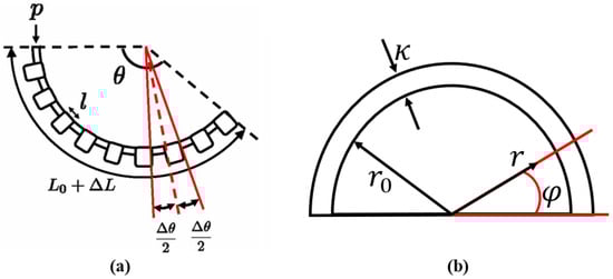
Figure 4. Physical structure of the soft robotic finger: (a) structural model; (b) cross section.

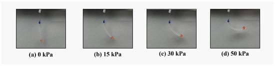
Figure 5. Bending soft robotic finger with different input pressures.

To derive the mathematical model of the soft robotic finger, the variables and parameters in Figure 4 are introduced. $\mathit{p}$ (kPa) denotes the input pressure; $\theta$ (rad) is the output bending angle. ${\mathit{L}}_0$ serves as the initial length of the finger and $\Delta L$ is the change during bending. $\mathit{l}$ denotes the length of each unit, while ${\mathit{r}}_0$ is the inner radius of each unit and $\kappa$ is the thickness of the rubber. According to the results in [28], the equations of moments are derived from the integral of elastic force and pressure within radius $[0,r]$ and angle $[0,\phi ]$, by which the mathematical model of the soft robotic finger can be written as

$$\theta =-{\displaystyle \frac{{\mathit{L}}_0}{\kappa }}\left(1+{\displaystyle \frac{2\mathit{R}+\kappa \pi }{\gamma \mathit{p}-2\mathit{R}-\kappa \pi }}\right)$$

(31)

$$\gamma ={\displaystyle \frac{4{\mathit{r}}_0^3+3\pi {\mathit{r}}_0^2\kappa }{6{\mathit{r}}_0\kappa {\mathit{E}}_0}}$$

(32)

where ${\mathit{E}}_0$ is the Young’s modulus and $\mathit{R}=r_0+{\displaystyle \frac{\kappa }{2}}$. It should be noted that the input pressure and output angle are physically constrained within $\mathit{p}\in \left[0,60\right],\theta \in \left[0,\pi \right]$. In the following analysis, Equation (31) will serve as the nominal plant for control design in comparative experiments.

4.2. Experimental Set up and Process

The experimental set up for the soft robotic finger and details of the process are introduced here. A visible overview of the experimental set up is exhibited in Figure 6, while the detailed process is shown in Figure 7.

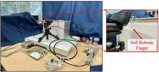
Figure 6. Overview of experimental set up.

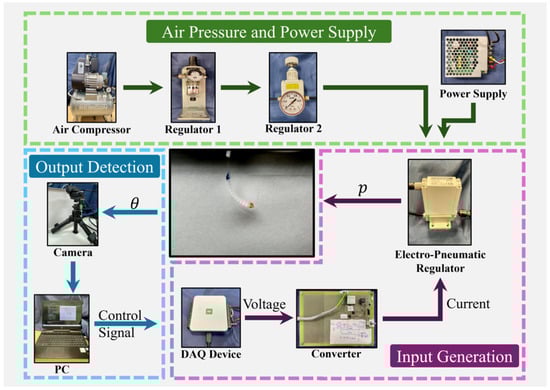
Figure 7. Experimental process.

Accordingly, one can find that the soft robotic finger and camera are placed on a vibration-isolated platform, which protects them from ground-induced vibration and perturbation. The air pressure is provided by a compressor, which is connected to two regulators. Specifically, regulator 1 is selected to filter out oil and dust, while the other (regulator 2) is involved in security by monitoring the pressure level. To realize the automatic control on the soft robotic finger, an electro-pneumatic regulator is selected, which is driven by an external power supply. The output pressure of the electro-pneumatic regulator is proportional to the input current, which is controlled by PC through a data acquisition (DAQ) device and a voltage–current converter. Finally, images of the soft robotic finger are collected by a camera, which contributes to the calculation of bending angle.

4.3. Neural Network Training and Controllers Design

To realize the proposed machine learning and operator-based nonlinear internal model control, a single-input single-output three-layer feedforward neural network trained via the back propagation (BP) algorithm is employed in this work for the establishment of the learning plant. According to the nominal model (31), the input–output relationship of the considered soft robotic finger is static, which makes it suitable to be approximated by a neural network. Firstly, the dataset is collected by setting the input pressure $\mathit{u}\left(t\right)=30+30sin\left({\displaystyle \frac{\pi }{20}}t\right)$, $\mathit{t}\in$ [0 s, 100 s] and the sampling time $\mathit{d}t=0.1$ s. As a result, 1000 samples are collected; 60% of them are used for training and 40% for validation.

Moreover, the structure of the neural network is depicted in Figure 8, where $\mathit{x}$ and $\mathit{y}$ denote the input and output of the plant, respectively. In order to achieve a good balance between approximation accuracy and computational complexity, based on multiple training trials, the rest of the neural network is configured as follows: $\mathit{k}=50$ neurons are selected in hidden layer, with weights ${\mathit{v}}_k$, ${\mathit{w}}_k$; ${\gamma }_k$ and $\rho$ denote the threshold of each neuron; the learning rate is set as 0.3, with 60 training iterations and a stopping threshold of $1\times {10}^{-5}$; the activation function is selected as

$$f\left(x\right)={\displaystyle \frac{1}{1+e^{-x}}}$$

(33)

and the loss functions are

$$\begin{array}{cc}\hfill J_{train}& ={\displaystyle \frac{1}{N_{train}}}\sum _{j=1}^{N_{train}}{({\widehat{y}}_j-y_j)}^2\hfill \end{array}$$

(34)

$$\begin{array}{cc}\hfill J_{val}& ={\displaystyle \frac{1}{N_{val}}}\sum _{j=1}^{N_{val}}{({\widehat{y}}_j-y_j)}^2\hfill \end{array}$$

(35)

where ${\mathit{N}}_{train}$ and ${\mathit{N}}_{val}$ denote the total number of training and validation samples; in addition, a coefficient of determination ${\mathit{R}}^2$ is formulated as follows to evaluate the precision of neural network prediction:

$$R^2=1-{\displaystyle \frac{{\sum }_{j=1}^{N_{val}}{({\widehat{y}}_j-y_j)}^2}{{\sum }_{j=1}^{N_{val}}{(y_j-\overline{y})}^2}}$$

(36)

where $\overline{y}={\displaystyle \frac{1}{N_{val}}}{\sum }_{j=1}^{N_{val}}{y}_j$.

Figure 8. Structure of neural network for soft robotic finger.

Finally, convergence of the loss functions during neural network training is shown in Figure 9, and the comparative results between the nominal plant, learning plant, and real plant are exhibited in Figure 10.

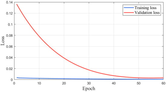
Figure 9. Convergence of the loss functions.

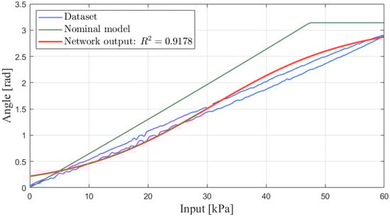
Figure 10. Outputs of nominal plant (dataset), learning plant (network output), and real plant.

It can clearly be observed from Figure 10 that the soft robotic finger performs hysteresis in the real world, which makes the nominal plant with output saturation less accurate to describe the dynamics. In contrast, one can see that the learning plant is closer to the real plant, with a precision of ${\mathit{R}}^2=0.9178$. This indicates the applicability of the obtained learning plant for nonlinear internal model control and is expected to result in better tracking performance.

For the next step, following the scheme described in Section 3, the controllers $\mathit{A}$, ${\mathit{A}}_0$, $\mathit{B}$, ${\mathit{B}}_0$ and $\mathit{C}$ will be designed. According to the operator theory in the RCF feedback system, the mathematical model (31) can be factorized into

$$\begin{array}{cc}\hfill \mathit{N}\left(\omega \right)\left(\mathit{t}\right)& =-{\displaystyle \frac{{\mathit{L}}_0}{\kappa }}\left(1+{\displaystyle \frac{2\mathit{R}+\kappa \pi }{\omega \left(\mathit{t}\right)-2\mathit{R}+\kappa \pi }}\right)\hfill \end{array}$$

(37)

$$\begin{array}{cc}\hfill {\mathit{D}}^{-1}\left(\mathit{u}\right)\left(\mathit{t}\right)& =\gamma ·\mathit{u}\left(\mathit{t}\right)\hfill \end{array}$$

(38)

To satisfy the Bezout Identity, $\mathit{A}$ and $\mathit{B}$ can be designed as

$$\begin{array}{cc}\hfill \mathit{A}\left({\mathit{y}}_0\right)\left(\mathit{t}\right)& =\left(1-\mathit{K}\right)\left(-{\displaystyle \frac{{\mathit{L}}_0(2\mathit{R}+\kappa \pi )}{\kappa {\mathit{y}}_0\left(\mathit{t}\right)+{\mathit{L}}_0}}+2\mathit{R}+\kappa \pi \right)\hfill \end{array}$$

(39)

$$\begin{array}{cc}\hfill \mathit{B}\left(\mathit{u}\right)\left(\mathit{t}\right)& =\gamma \mathit{K}·\mathit{u}\left(\mathit{t}\right)\hfill \end{array}$$

(40)

where $\mathit{K}$ is an designed parameter and is selected as $\mathit{K}=1.25$ in this work. As a result, one can find $\mathit{A}N+BD=I$ based on (37)–(39), which suggests the robust stability of the RRCF feedback system. Moreover, to coincide with the concept of internal model control, $\mathit{C}$ is designed as $\mathit{C}=N^{-1}$.

Additionally, to explore the feasibility of the neuron network based on the RRCF feedback loop, i.e., the flow from $\tilde{e}\left(t\right)$ towards $\widehat{y}$ in Figure 3, a simulation verification is conducted. The simulated results are exhibited in Figure 11, where stable outputs are obtained from bounded external input $\tilde{e}\left(t\right)=1.4+0.8/e^{-9t+90}$. Hence, the neuron network-based RRCF feedback loop is considered safe for further practical implementation.

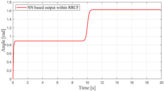
Figure 11. Simulated results of neuron network-based output within RRCF.

4.4. Experimental Results

Comparative experiments are conducted between the machine learning-based IMC system (the proposed method) and the IMC system in [25] with PI/PD controllers. The reference input is set as

$$\tilde{r}\left(t\right)=1.4+{\displaystyle \frac{0.8}{e^{-9t+90}}}$$

(41)

and the total experiment period is 20 s. Moreover, according to the aforementioned parameter ranges of (22) and multiple experimental trials conducted under various scenarios, specific parameters selected for different controllers are listed in Table 1.

Table 1. Parameters selection in different scenarios.

Control Method	Parameters
NN-based IMC	${\mathit{K}}_P=-0.6$, ${\mathit{K}}_I=0.085$
IMC with PI controller	${\mathit{K}}_P=-0.6$, ${\mathit{K}}_I=0.02$
IMC with PD controller	${\mathit{K}}_P=-0.6$, ${\mathit{K}}_D=0.001$

The visible results from different scenarios can be found in Figure 12, Figure 13, Figure 14 and Figure 15. It is observed in Figure 12 that, when the target value is relatively lower, each method produces outputs that track the target. In contrast, despite implementing the PI/PD controller, the outputs of a normal IMC-based system cannot converge to the higher reference, due to the output saturation and larger difference between the internal model and the real plant. This claim is further supported by Figure 13. The tracking errors in different scenarios converge to zero when the reference is $\tilde{r}(·)=1.4$ rad, while the ones using normal IMC perform a tracking error of $-0.2$ for reference $\tilde{r}(·)=2.2$ rad. Such a difference in tracking errors verifies the essential role of the machine learning plant in this framework.

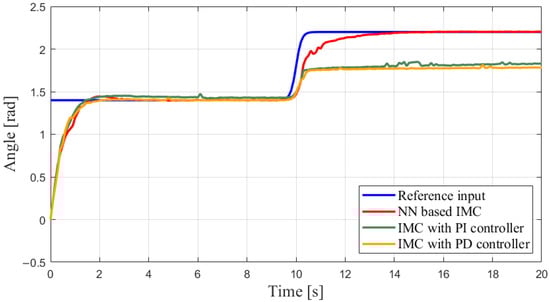
Figure 12. Outputs comparison in different scenarios.

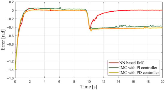
Figure 13. Tracking errors in different scenarios.

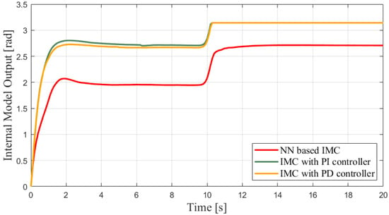
Figure 14. Outputs of internal model in different scenarios.

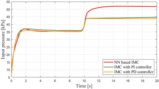
Figure 15. Input pressure in different scenarios.

The outputs of the internal model $\widehat{y}$ can be found in Figure 14. The saturation after 10 s also indicates the negative influence on the control performance when using an imprecise mathematical model. In other words, this suggests the necessity of implementing the machine learning plant to prevent avoidable saturation, as well as the effectiveness of inserting a machine learning plant into an IMC framework. Finally, the input pressures in different scenarios are exhibited in Figure 15. Besides the neural network, a support vector regression (SVR)-based machine learning plant is implemented into the proposed framework, and the experimental results are exhibited in Figure 16, which further supports the feasibility of the ML-based IMC design.

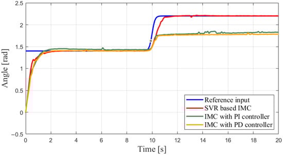
Figure 16. Outputs comparison in different scenarios while using SVR.

5. Conclusions

In this work, the practical implementation of machine learning models in a real-world control system is addressed. Although the obtained learning plant lacks mathematical dynamic formulation, the bounded input/output spaces are ensured using an RRCF feedback structure. In addition to stability, the tracking performance is investigated under a nonlinear IMC architecture. The proposed framework is then applied to a soft robotic finger system. According to the results, one can find superior performance when using ML-based IMC, since a more precise learning model avoids negative saturation. Such a finding also implies the feasibility of the proposed framework and the requirement of learning plants in some cases.

Moreover, the proposed framework is considered to be of far-reaching significance. By leveraging RRCF, the learning plants can be inserted as long as they satisfy the conditions on input/output spaces, even with the existence of perturbation or finite jumps. Future research will address ML-based enhancement on controller design, considering stability and security in practice.

References

- Meng, L.; Hirayama, T.; Oyanagi, S. Underwater-drone with panoramic camera for automatic fish recognition based on deep learning. IEEE Access 2018, 6, 17880–17886. [Google Scholar] [CrossRef]
- Yue, X.; Meng, L. YOLO-MSA: A multi-scale stereoscopic attention network for empty-dish recycling robots. IEEE Trans. Instrum. Meas. 2023, 72, 2528014. [Google Scholar] [CrossRef]
- Ge, Y.; Li, Z.; Yue, X.; Li, H.; Li, Q.; Meng, L. IoT-based automatic deep learning model generation and the application on empty-dish recycling robots. Internet Things 2024, 25, 101047. [Google Scholar] [CrossRef]
- Mahadevkar, S.; Khemani, B.; Patil, S.; Kotecha, K.; Vora, D.; Abraham, A.; Gabralla, L. A review on machine learning styles in computer vision—techniques and future directions. IEEE Access 2022, 10, 107293–107329. [Google Scholar] [CrossRef]
- Chen, S.; Billings, S.; Grant, P. Non-linear system identification using neural networks. Int. J. Control 1990, 51, 1191–1214. [Google Scholar] [CrossRef]
- Wang, J.; Chen, Y. A fully automated recurrent neural network for unknown dynamic system identification and control. IEEE Trans. Circuits Syst. I Regul. Pap. 2006, 53, 1363–1372. [Google Scholar] [CrossRef]
- Chiuso, A.; Pillonetto, G. System identification: A machine learning perspective. Annu. Rev. Control. Robot. Auton. Syst. 2019, 2, 281–304. [Google Scholar] [CrossRef]
- Patino, H.; Carelli, R.; Kuchen, B. Neural networks for advanced control of robot manipulators. IEEE Trans. Neural Netw. 2002, 13, 343–354. [Google Scholar] [CrossRef] [PubMed]
- Lee, T.; Christopher, J. Adaptive Neural Network Control of Robotic Manipulators; World Scientific: Singapore, 1998. [Google Scholar]
- Dikici, O.; Ghignone, E.; Hu, C.; Baumann, N.; Xie, L.; Carron, A. Learning-based on-track system identification for scaled autonomous racing in under a minute. IEEE Robot. Autom. Lett. 2025, 10, 1984–1991. [Google Scholar] [CrossRef]
- Soori, M.; Arezoo, B.; Dastres, R. Artificial intelligence, machine learning and deep learning in advanced robotics, a review. Cogn. Robot. 2023, 3, 54–70. [Google Scholar] [CrossRef]
- Semeraro, F.; Griffiths, A.; Cangelosi, A. Human–robot collaboration and machine learning: A systematic review of recent research. Robot. Comput.-Integr. Manuf. 2023, 79, 102432. [Google Scholar] [CrossRef]
- Wang, D.; Dang, G. Fuzzy recurrent stochastic configuration networks for industrial data analytics. IEEE Trans. Fuzzy Syst. 2024, 33, 1178–1191. [Google Scholar] [CrossRef]
- Rivals, I.; Personnaz, L. Nonlinear internal model control using neural networks: Application to processes with delay and design issues. IEEE Trans. Neural Netw. 2000, 11, 80–90. [Google Scholar] [CrossRef] [PubMed]
- Bonassi, F.; Scattolini, R. Recurrent neural network-based internal model control design for stable nonlinear systems. Eur. J. Control 2022, 65, 100632. [Google Scholar] [CrossRef]
- Huang, J.; Lewis, F. Neural-network predictive control for nonlinear dynamic systems with time-delay. IEEE Trans. Neural Netw. 2003, 14, 377–389. [Google Scholar] [CrossRef]
- Zhou, X.; Wang, W.; Shi, Y. Neural network/PID adaptive compound control based on RBFNN identification modeling for an aerial inertially stabilized platform. IEEE Trans. Ind. Electron. 2024, 71, 16514–16522. [Google Scholar] [CrossRef]
- Huang, K.; Wei, K.; Li, F.; Yang, C.; Gui, W. LSTM-MPC: A deep learning based predictive control method for multimode process control. IEEE Trans. Ind. Electron. 2023, 70, 11544–11554. [Google Scholar] [CrossRef]
- Bu, N.; Zhang, Y.; Li, X.; Chen, W.; Jiang, C. Passive robust control for uncertain Hamiltonian systems by using operator theory. CAAI Trans. Intell. Technol. 2022, 7, 594–605. [Google Scholar] [CrossRef]
- Bu, N.; Zhang, Y.; Li, X. Robust tracking control for uncertain micro hand actuator with Prandtl-Ishlinskii hysteresis. Int. J. Robust Nonlinear Control 2023, 33, 9391–9405. [Google Scholar] [CrossRef]
- Katsurayama, Y.; Deng, M.; Jiang, C. Operator-based experimental studies on nonlinear vibration control for an aircraft vertical tail with considering low-order modes. Trans. Inst. Meas. Control 2015, 38, 1421–1433. [Google Scholar] [CrossRef]
- Takahashi, K.; Deng, M. Nonlinear sensorless cooling control for a Peltier actuated aluminum plate thermal system. In Proceedings of the 2013 International Conference on Advanced Mechatronic Systems, Luoyang, China, 25–27 September 2013; pp. 1–6. [Google Scholar]
- Usami, T.; Deng, M. Applying an MSVR method to forecast a three-degree-of-freedom soft actuator for a nonlinear position control system: Simulation and experiments. IEEE Syst. Man Cybern. Mag. 2022, 8, 61–69. [Google Scholar] [CrossRef]
- An, Z.; Deng, M. Learning and operator based control system design for soft robotic finger with denial of service attack and input hysteresis using right coprime factorization. In Proceedings of the 6th International Conference on Industrial Artificial Intelligence, Shenyang, China, 21–24 August 2024; pp. 1–6. [Google Scholar]
- Jin, G.; Deng, M. Non-linear forced vibration control for a vertical wing-plate with sustainable perturbation by using internal model control mechanism. Int. J. Control 2023, 96, 1543–1550. [Google Scholar] [CrossRef]
- Lakshmikantham, V.; Bainov, D.; Simeonov, P. Theory of Impulsive Differential Equations; World Scientific: Singapore, 1989. [Google Scholar]
- An, Z.; Deng, M.; Morohoshi, Y. Right coprime factorization-based simultaneous control of input hysteresis and output disturbance and its application to soft robotic finger. Electronics 2024, 13, 2025. [Google Scholar] [CrossRef]
- Fujita, K.; Deng, M.; Wakimoto, S. A miniature pneumatic bending rubber actuator controlled by using the PSO-SVR-based motion estimation method with the generalized Gaussian kernel. Actuators 2017, 6, 6. [Google Scholar] [CrossRef]
Disclaimer/Publisher’s Note: The statements, opinions and data contained in all publications are solely those of the individual author(s) and contributor(s) and not of MDPI and/or the editor(s). MDPI and/or the editor(s) disclaim responsibility for any injury to people or property resulting from any ideas, methods, instructions or products referred to in the content. |
© 2026 by the authors. Licensee MDPI, Basel, Switzerland. This article is an open access article distributed under the terms and conditions of the Creative Commons Attribution (CC BY) license.