Semantic-Guided Kernel Low-Rank Sparse Preserving Projections for Hyperspectral Image Dimensionality Reduction and Classification

Abstract

Hyperspectral images present significant challenges for conventional dimensionality reduction methods due to their high dimensionality, spectral redundancy, and complex spatial–spatial dependencies. While kernel-based sparse representation methods have shown promise in handling spectral non-linearities, they often fail to preserve spatial consistency and semantic discriminability during feature transformation. To address these limitations, we propose a novel semantic-guided kernel low-rank sparse preserving projection (SKLSPP) framework. Unlike previous approaches that primarily focus on spectral information, our method introduces three key innovations: a semantic-aware kernel representation that maintains discriminability through label constraints, a spatially adaptive manifold regularization term that preserves local pixel affinities in the reduced subspace, and an efficient optimization framework that jointly learns sparse codes and projection matrices. Extensive experiments on benchmark datasets demonstrate that SKLSPP achieves superior performance compared to state-of-the-art methods, showing enhanced feature discrimination, reduced redundancy, and improved robustness to noise while maintaining spatial coherence in the dimensionality-reduced features.

1. Introduction

Hyperspectral imaging (HSI) technology has revolutionized remote sensing by providing detailed spectral information across hundreds of contiguous bands, thus enabling precise material identification and classification [1,2]. This rich spectral characterization, however, comes with significant challenges, including the well-known curse of dimensionality [3], spectral redundancy [4], and complex non-linear mixing phenomena [5]. These issues necessitate effective dimensionality reduction (DR) techniques capable of transforming high-dimensional hyperspectral data into more compact and discriminative representations while simultaneously preserving essential spectral–spatial characteristics.

It is often acknowledged that images lie on a low-dimensional manifold, whose intrinsic structure can be effectively captured through manifold learning-based DR techniques [6]. Traditional linear approaches such as principal component analysis (PCA) [7], independent component analysis (ICA) [8], and linear discriminant analysis (LDA) [9] have been widely adopted but are limited in their ability to characterize the non-linear structures inherent in HSI data. To address this limitation, non-linear manifold learning techniques have been introduced, including kernel discriminant analysis (KDA) [10], Laplacian eigenmaps [11], neighborhood preserving embedding [12], locality linear embedding [13], and locality preserving projection (LPP) [14]. These methods attempt to preserve the local geometric structure of data in a reduced subspace. Building upon these foundations, Sugiyama [15] proposed local Fisher discriminant analysis, which combines LPP and LDA to enhance discriminative power while maintaining local structural preservation. Yan et al. [16] further advanced the field by establishing a unified graph embedding framework that generalizes various DR methods. Subsequent developments incorporated sparsity constraints into this framework. For instance, Cheng et al. [17] established the sparse graph embedding (SGE) model by incorporating HSI sparsity priors. To enhance land cover identification capabilities, Ly et al. [18] introduced a semi-supervised extension, sparse graph-based discriminant analysis, which integrates label information into graph construction.

However, despite these advancements, sparse representation methods primarily focus on achieving the sparsest reconstruction of individual samples, often overlooking semantic guidance during the learning process. In contrast to sparse representation approaches, low-rank representation (LRR) has emerged as a powerful framework for capturing global structures and handling data corruptions in high-dimensional domains [19,20]. The fundamental premise is that data samples from multiple subspaces can be represented as linear combinations of dictionary bases, resulting in a low-rank coefficient matrix that reveals global subspace membership. This paradigm demonstrates remarkable robustness to various corruptions, including noise, outliers, and occlusions, as evidenced by its successful applications in diverse domains such as face recognition [21], motion segmentation [22], and hyperspectral image analysis [23].

The theoretical foundation of LRR was significantly advanced by Liu et al. [20], who established robust subspace recovery through nuclear norm minimization. Subsequent developments have extended LRR in several directions that are particularly relevant to HSI analysis. For instance, Zhang et al. [24] introduced discriminative LRR that incorporates label information to enhance class separability. Similarly, Wong et al. [25] embedded low-rank constraints into orthogonal subspaces to reduce corruption impacts. Chen et al. [26] developed symmetric LRR constraints that improve representation accuracy. Furthermore, Du et al. [27] integrated low-rank representation with adaptive manifold learning to simultaneously capture local and global structures. While low-rank representation methods effectively capture global structures, they often overlook valuable local spatial information within and between classes. This is a critical aspect for hyperspectral image analysis, as adjacent pixels frequently share material compositions. This limitation has prompted research into methods that integrate discriminative and structural constraints. Jiang et al. [28] proposed Laplacian regularized collaborative representation projection (LRCRP) for unsupervised hyperspectral DR. LRCRP combines Laplacian regularization and local enhancement within collaborative representation to preserve local–global structures, thereby effectively exploring collaborative relationships among features.

Despite these advancements, current DR methods for HSI suffer from three fundamental limitations that hinder their effectiveness. First, they often neglect semantic consistency during feature transformation, leading to weakened discriminative power in the reduced subspace. Second, most approaches assume linear separability, which cannot adequately capture the complex non-linear relationships inherent in hyperspectral data. Third, existing methods frequently ignore crucial spatial neighborhood structures that provide complementary information to spectral features. This is particularly problematic for HSI analysis, as adjacent pixels often share similar material compositions. These limitations collectively result in suboptimal performance, characterized by weak semantic knowledge acquisition and the unrealized full potential of hyperspectral data.

To bridge these critical gaps and leverage the complementary strengths of both sparse and low-rank paradigms, we propose a novel semantic-guided kernel low-rank sparse preserving projection (SKLSPP) framework for hyperspectral image DR. The main contributions of this work are summarized as follows:

(1)

Semantic-aware kernel sparse representation. We propose a semantic guidance mechanism that integrates label information directly into the kernel sparse representation learning framework. This mechanism explicitly preserves semantic consistency during feature transformation via discriminative constraints in the kernel-induced feature space.

(2)

Spatially adaptive manifold regularization. We introduce a dynamically weighted graph Laplacian regularization term that captures both spectral similarity and spatial proximity among pixels. This adaptive manifold construction effectively preserves the local geometric structure of hyperspectral data while also accommodating the unique characteristics of different land cover types and overcoming the limitations of fixed neighborhood representations in conventional manifold learning methods.

(3)

Unified optimization framework with efficient computation. We establish a comprehensive optimization framework that jointly learns the sparse codes, projection matrix, and manifold structure through an iterative algorithm combining generalized power iteration and augmented Lagrangian methods.

By bridging the gaps between sparse representation, low-rank learning, and manifold embedding in a kernel-based framework, our approach offers a principled solution for extracting compact yet highly discriminative features from complex hyperspectral imagery. The remainder of this paper is organized as follows. Section 2 and Section 3 provide the theoretical background and detailed formulation of the proposed SKLSPP framework. Section 4 presents extensive experimental results and comparative analysis on benchmark hyperspectral datasets. Finally, Section 5 concludes the paper with a summary of the key findings and potential future research directions.

2. Theoretical Background

2.1. Sparse Representation

Assume that there is a set of samples from HSI, $X=\left[x_1,x_2,...,x_N\right]\in {\mathbb{R}}^{D\times N}$, where $D$ is the spectral dimension and $N$ is the total number of pixels. Provide a dictionary $Q=\left[q_1,q_2,...,q_K\right]\in {\mathbb{R}}^{D\times K}$, where $K$ is the number of atoms in the dictionary and each $q_i\in {\mathbb{R}}^D$ represents a basic spectral signature. For an arbitrary pixel $x\in {\mathbb{R}}^D$, the goal of sparse representation (SR) is to find a sparse coefficient vector ${s=\left[s_1,s_2,...,s_K\right]}^T\in {\mathbb{R}}^K$ such that $x\approx Qs$. The sparseness of $s$ is typically enforced by minimizing its ${\mathcal{l}}_0$-norm or ${\mathcal{l}}_1$-norm. The ${\mathcal{l}}_0$-norm counts the number of non-zero elements in $s$, while the ${\mathcal{l}}_1$-norm is its convex relaxation, which is computationally more tractable. Then, the sparse representation problem can be formulated as follows:

$$\underset{s}{\min }{\Vert s\Vert }_1 s.t. {\Vert x-Qs\Vert }_2^2 \le ϵ$$

where ${\Vert ·\Vert }_1$ is ${\mathcal{l}}_1$-norm and $ϵ$ is a small positive constant that controls the reconstruction error. The dictionary $Q$ can be constructed in various ways. In many applications, the training samples themselves are used as the dictionary, i.e., $Q=X$.

2.2. Low-Rank Representation

Following the understanding of local manifold structures provided by SR, low-rank representation (LRR) emerges as a complementary and often more robust technique, particularly when dealing with complex HSI data corrupted by various interferences. Given a dataset $X=\left[x_1,x_2,...,x_N\right]\in {\mathbb{R}}^{D\times N}$, LRR seeks to find a coefficient matrix $Z\in {\mathbb{R}}^{N\times N}$, such that $X\approx XZ$ and $Z$ has a low rank. The objective function for LRR is typically formulated as follows:

$$\underset{Z}{\mathit{min}}\Vert Z{\Vert }_{*} s.t. X=XZ$$

where $\Vert Z{\Vert }_{*}$ denotes the nuclear norm of $Z$, which is a convex surrogate for the rank function. In practice, to account for noise, outliers, and corruptions inherent in real-world HSI data, the objective can be modified to explicitly handle these disturbances as follows:

$$\underset{Z,\mathit{E}}{\min }\Vert Z{\Vert }_{*}+\lambda {\Vert E\Vert }_{2,1}s.t. X=XZ+E$$

Here, $E$ represents the error or corruption matrix. The ${\mathcal{l}}_{2,1}$-norm of $E$ promotes column-wise sparsity. The parameter $\lambda >0$ balances the nuclear norm of $Z$ and the ${\mathcal{l}}_{2,1}$-norm of $E$.

2.3. Low-Rank Sparse Preserving Projections

In Ref. [29], Xie et al. propose low-rank sparse preserving projections for dimensionality reduction (LSPP) that unify low-rank, sparse, and manifold preservation. Mathematically, LSPP can be expressed as

$$\underset{P,Z,E}{\min }\Vert Z{\Vert }_{*}+\alpha {\Vert Z\Vert }_1+\beta {\Vert E\Vert }_{\mathrm{2,1}}+\lambda \mathrm{t}\mathrm{r}(P^{T}XM{X}^{T}P) s.t. P^{T}X=P^{T}XZ+E$$

Its objective typically includes a term $\mathrm{t}\mathrm{r}\left(P^{T}XM{X}^{T}P\right)$, where $P$ is a projection matrix that maps high-dimensional data to a low-dimensional space and $M$ is a Laplacian matrix from a neighborhood graph. This term maintains local topological structure by ensuring points close in $X$ remain close in the projected space. $\alpha$, $\beta$,$\mathrm{a}\mathrm{n}\mathrm{d} \lambda$ are tradeoff parameters that balance the sparsity, low-rankness, and manifold term.

Despite its advancements, LSPP faces two primary limitations, particularly for complex HSI analysis. Firstly, its linear projection nature hinders its ability to capture the inherent non-linear structures and relationships within HSI data. Secondly, the manifold-preserving term relies on a static Laplacian matrix from a fixed neighborhood graph, precluding adaptation to evolving semantic relationships between classes and thus impeding optimal class separation during iterative learning.

To overcome these shortcomings and achieve more robust and discriminative dimensionality reduction for HSI, this paper proposes a novel framework that (1) leverages kernel methods to implicitly handle non-linear structures, mapping data into a high-dimensional feature space where linear separability is enhanced and (2) introduces a dynamic inter-class constraint, explicitly incorporating prior class label information into the optimization. This constraint, inspired by [30], enables the model to adaptively emphasize and refine inter-class semantic relationships throughout the iterative learning process, ensuring stronger class separability in the learned low-dimensional representation.

3. Methodology

This section details the proposed SKLSPP for DR. We first introduce kernel mapping to address the non-linear nature of HSI. Subsequently, a novel semantic-guided constraint is integrated to enhance inter-class separability by leveraging prior label information.

3.1. Kernel Low-Rank Sparse Preserving Projection (KLSPP)

LSPP is designed to find a low-dimensional subspace that simultaneously preserves data locality and global structural information through sparse reconstruction. However, HSI data often exhibit complex non-linear manifolds that linear projection models, like conventional LSPP, may fail to capture effectively. To address this, we extend LSPP into its kernelized form.

Let $X=\left[x_1,x_2,...,x_{N_L}\right]\in {\mathbb{R}}^{D\times N_L}$ be the matrix of $N_L$ labeled training samples and $Y=\left[y_1,y_2,...,y_{N_U}\right]\in {\mathbb{R}}^{D\times N_U}$ be the matrix of $N_U$ unlabeled test samples, where $D$ is the original spectral dimensionality. Let $\mathsf{\Phi }:{\mathbb{R}}^D\to \mathcal{H}$ be a non-linear mapping function that projects the original data from the input space to a high-dimensional space $\mathcal{H}$. The inner product in this feature space is implicitly defined by a chosen kernel function $k$.

$$k(x_i,x_j)=⟨\mathsf{\Phi }\left(x_i\right),\mathsf{\Phi }\left(x_j\right)⟩$$

(1)

In this high-dimensional space, our objective is to learn a low-dimensional projection that captures the intrinsic structure of the data. Following the representer theorem, the optimal projection matrix $P\in {\mathbb{R}}^{\widehat{D}\times d}$ (where $\widehat{D}$ is the potentially infinite dimension) in the feature space $\mathcal{H}$ can be expressed as a linear combination of the mapped training samples as follows:

$$P={\sum }_{i=1}^{N_L}\mathsf{\Phi }\left(x_i\right)a_i=\mathsf{\Phi }\left(X\right)A$$

(2)

where $A\in {\mathbb{R}}^{N_L\times d}$ is the coefficient matrix we aim to learn. Each column of $A$ corresponds to the coefficients for a specific projection direction in $\mathcal{H}$ and $d$ is the desired reduced dimensionality. Thus, our primary goal is to optimize $A$ to define this effective projection.

The low-dimensional projections of the training samples $X$ and test samples $Y$ can then be obtained by applying this projection operator $P$. By substituting Equation (2) and employing the kernel trick (Equation (1)), we can avoid explicit computation in the high-dimensional space $\mathcal{H}$ as follows:

$$P^T\mathsf{\Phi }\left(X\right)={\left(\mathsf{\Phi }\right(X\left)A\right)}^T\mathsf{\Phi }\left(X\right)=A^T{\mathsf{\Phi }\left(X\right)}^T\mathsf{\Phi }\left(X\right)=A^T{K}_{XX}$$

(3)

$$P^T\mathsf{\Phi }\left(Y\right)={\left(\mathsf{\Phi }\right(X\left)A\right)}^T\mathsf{\Phi }\left(Y\right)=A^T{\mathsf{\Phi }\left(X\right)}^T\mathsf{\Phi }\left(Y\right)=A^T{K}_{XY}$$

(4)

where $K_{XX}\in {\mathbb{R}}^{N_L\times N_L}$ is the kernel matrix computed between all pairs of training samples $X$, i.e., ${\left(K_{XX}\right)}_{ij}=k(x_i,x_j)$. Similarly, $K_{XY}\in {\mathbb{R}}^{N_L\times N_U}$ is the cross-kernel matrix between training samples $X$ and test samples $Y$, i.e., ${\left(K_{XY}\right)}_{ij}=k(x_i,y_j)$.

Incorporating these components and applying the kernel trick, the objective function for KLSPP is formulated as follows:

$$\begin{gathered} \underset{A,Z}{min} {\Vert A^T{K}_{XY}-A^T{K}_{XX}Z\Vert }_F^2+\alpha {\Vert Z\Vert }_{2, 1}+\lambda \mathrm{T}\mathrm{r}\left(A^T{K}_{XX}M{K}_{XX}A\right) \\ s.t. A^T{K}_{XX}A=\mathrm{I} \end{gathered}$$

(5)

where $A^T{K}_{XX}A=\mathrm{I}$ is the kernelized orthogonality constraint, ensuring that the projection basis is orthonormal in the kernel space, thereby preventing trivial solutions and preserving the variance of the data. The term ${\Vert A^T{K}_{XY}-A^T{K}_{XX}Z\Vert }_F^2$ aims to learn a low-rank representation $Z$ that links the projections of samples, serving to capture the underlying relationships between the projected training samples and test samples. The Laplacian matrix $M\in {\mathbb{R}}^{N_L\times N_L}$ is defined as $M=D_X-W_X$, where $W_X$ is a similarity matrix of $X$ and $D_X$ is a diagonal matrix with $D_{X, ii}={\sum }_j{W}_{X, ij}$. This term encourages samples that are close in the original feature space to remain close in the projected space. $\alpha$ and $\lambda >0$ are regularization parameters.

3.2. Semantic-Guided Kernel Low-Rank Sparse Preserving Projection (SKLSPP)

To further enhance the discriminative power of the learned features and infuse prior semantic knowledge into the projection process, we strategically incorporate an intra-class regularization term within the SKLSPP framework. This term specifically aims to strengthen the correlation among samples belonging to the same class in the projected subspace. Let $L\in \{\mathrm{0,1}{\}}^{N_L\times C}$ be a one-hot matrix, where $N_L$ denotes the number of training samples and $C$ is the total number of classes. For any training sample $x_i$ belonging to class $c$, its corresponding entry in $L$ is $L_{ic}=1$, while $L_{ij}=0$ for $j\ne c$. The product $P^T\mathsf{\Phi }\left(X\right)L={\mathrm{A}}^T{K}_{XX}L$ then represents the class-wise averaged low-dimensional embeddings of the training samples. Each column of ${\mathrm{A}}^T{K}_{XX}L$ effectively provides a consolidated representation for a specific class, capturing the central tendency of its embedded samples, which in turn strengthens semantic consistency.

To encourage these class representations to exhibit strong internal coherence and a compact structure, we propose to minimize the nuclear norm of this class-wise averaged embedding term. This leads to the following constraint:

$$min\Vert {\mathrm{A}}^T{K}_{XX}L{\Vert }_{*}$$

(6)

Minimizing the nuclear norm of $\Vert {\mathrm{A}}^T{K}_{XX}L{\Vert }_{*}$ is a powerful mechanism that directly enforces a low-rank intrinsic structure within these class-wise averaged representations. This operation compels the projected data within each class to be not only highly correlated but also to reside within a minimal low-dimensional subspace. Consequently, this significantly enhances intra-class compactness and crucially improves inter-class separability in the reduced-dimensional space. This mechanism provides potent semantic guidance by inherently ensuring that samples from the same class are projected into a more cohesive, distinctive, and semantically consistent region, directly addressing the challenge of preserving meaningful class structures during dimensionality reduction.

By strategically combining this semantic-guided low-rank constraint (Equation (6)) with the original KLSPP objective function from Equation (5), our final proposed model, semantic-guided kernel low-rank sparse preserving projection (SKLSPP), is formulated as follows:

$$\begin{gathered} \underset{A, Z}{min} {\Vert A^T{K}_{XY}-A^T{K}_{XX}Z\Vert }_F^2+\alpha {\Vert Z\Vert }_{2, 1}+{\lambda }_1\Vert A^T{K}_{XX}L{\Vert }_{*}+{\lambda }_2\mathrm{T}\mathrm{r}\left(A^T{K}_{XX}M{K}_{XX}A\right) \\ s.t. A^T{K}_{XX}A=\mathrm{I} \end{gathered}$$

(7)

where $\alpha ,$ ${\lambda }_1$, and ${\lambda }_2$ are regularization parameters controlling the weight of each term. This comprehensive objective function integrates sparse reconstruction of test data, robust sparsity regularization, semantic-guided class separation, and local manifold preservation, all within a kernelized framework.

3.3. Optimization

The objective function in Equation (7) is non-convex and involves multiple coupled variables with non-smooth norms, making its direct optimization challenging. We adopt the alternating direction method of multipliers (ADMM) for such problems. ADMM iteratively optimizes each variable while fixing the others, guaranteeing convergence to a local optimum. To decouple the variables and facilitate ADMM, we introduce auxiliary variables $B$, $J$, and $G$. The problem in Equation (7) can be rewritten with auxiliary variables and corresponding constraints as follows:

$$\begin{gathered} \underset{A,Z,B, J,G}{min} {\Vert A^T{K}_{XY}-G\Vert }_F^2+\alpha {\Vert B\Vert }_{2, 1}+{\lambda }_1\Vert J{\Vert }_{*}+{\lambda }_2\mathrm{T}\mathrm{r}\left(A^T{K}_{XX}M{K}_{XX}A\right) \\ {s.t.A}^T{K}_{XX}A=\mathrm{I}, \\ Z-B=0 \\ { A}^T{K}_{XX}L-J=0, \\ { A}^T{K}_{XX}Z-G=0 \end{gathered}$$

(8)

The augmented Lagrangian function for this problem can be formulated as follows:

$$\begin{array}{c}L(A,Z,B,J,G,{\mathrm{\Lambda }}_1,{\mathrm{\Lambda }}_2,{\mathrm{\Lambda }}_3)={\Vert A^T{K}_{XY}-G\Vert }_F^2+\alpha {\Vert B\Vert }_{2, 1}+{\lambda }_1\Vert J{\Vert }_{*}+{\lambda }_2\mathrm{Tr}(A^T{K}_{XX}M{K}_{X}A)\\ +\mathrm{Tr}\left({\mathrm{\Lambda }}_1^T\left(Z-B\right)\right)+{\displaystyle \frac{\mu }{2}}{\Vert Z-B\Vert }_F^2\\ +\mathrm{Tr}\left({\mathrm{\Lambda }}_2^T(A^T{K}_{XX}L-J)\right)+{\displaystyle \frac{\mu }{2}}{\Vert A^T{K}_{XX}L-J\Vert }_F^2\\ +\mathrm{Tr}({\mathrm{\Lambda }}_3^T(A^T{K}_{XX}Z-G))+{\displaystyle \frac{\mu }{2}}{\Vert A^T{K}_{XX}Z-J\Vert }_F^2\end{array}$$

(9)

where ${\mathrm{\Lambda }}_1,{\mathrm{\Lambda }}_2,{\mathrm{\Lambda }}_3$ are Lagrangian multiplier matrices for the respective constraints, and $\mu > 0$ is a penalty parameter. The ADMM algorithm proceeds by iteratively updating each variable while holding the others fixed, followed by updating the Lagrangian multipliers and the penalty parameter.

(1)

Update A

When $Z^{\left(k\right)},B^{\left(k\right)},J^{\left(k\right)},G^{\left(k\right)},{\mathrm{\Lambda }}_1^{\left(k\right)},{\mathrm{\Lambda }}_2^{\left(k\right)},{\mathrm{\Lambda }}_3^{\left(k\right)}$ are fixed at their $k\mathrm{-th}$ iteration values, the subproblem for $A$ at iteration $k + 1$ is as follows:

$$\begin{gathered} \underset{A}{min}\mathrm{T}\mathrm{r}(A^T(K_{XY}{K}_{XY}^T+{\lambda }_2{K}_{XX}M{K}_{XX}+{\displaystyle \frac{\mu }{2}}{K}_{XX}L{L}^T{K}_{XX}^T+{\displaystyle \frac{\mu }{2}}{K_{XX}Z}^{\left(k\right)}{Z}^{\left(k\right)T}{K}_{XX}^T)A) \\ +\mathrm{T}\mathrm{r}({\mathrm{A}}^T\left(-2K_{XY}{G}^{\left(k\right)}-\mu K_{XX}L{(J^{\left(k\right)}-{\displaystyle \frac{{\mathrm{\Lambda }}_2^{\left(k\right)}}{\mu }})}^T-\mu K_{XX}{Z}^{\left(k\right)}{(G^{\left(k\right)}-{\displaystyle \frac{{\mathrm{\Lambda }}_3^{\left(k\right)}}{\mu }})}^T\right)) \\ \mathrm{s}.\mathrm{t}.A^T{K}_{XX}A=\mathrm{I} \end{gathered}$$

(10)

Combining all constant terms as $F_1^{\left(k\right)}$ and $F_2^{\left(k\right)}$, we define

$$F_1=K_{XY}{K}_{XY}^T+{\lambda }_2{K}_{XX}M{K}_{XX}+{\displaystyle \frac{\mu }{2}}{K}_{XX}L{L}^T{K}_{XX}^T+{\displaystyle \frac{\mu }{2}}{K}_{XX}{Z}^{\left(k\right)}{Z}^{\left(k\right)T}{K}_{XX}^T$$

(11)

$$F_2=-2K_{XY}{G}^{\left(k\right)}-\mu K_{XX}L{(J^{\left(k\right)}-{\displaystyle \frac{{\mathrm{\Lambda }}_2^{\left(k\right)}}{\mu }})}^T-\mu K_{XX}{Z}^{\left(k\right)}{(G^{\left(k\right)}-{\displaystyle \frac{{\mathrm{\Lambda }}_3^{\left(k\right)}}{\mu }})}^T$$

(12)

Then, Equation (10) can be reformulated as follows:

$$\underset{A}{min}\mathrm{T}\mathrm{r}(A^T{F}_{1}A)+\mathrm{T}\mathrm{r}(A^T{F}_2),\mathrm{s}.\mathrm{t}.A^T{K}_{XX}A=\mathrm{I}$$

(13)

To solve this problem, we introduce Lagrange multipliers $\mathrm{\Gamma }$. The augmented Lagrange function is as follows:

$$\mathcal{L}(A,\mathrm{\Gamma })=\mathrm{T}\mathrm{r}(A^T{F}_1^{\left(k\right)}A)+\mathrm{T}\mathrm{r}(A^T{F}_2^{\left(k\right)})+\mathrm{T}\mathrm{r}(\mathrm{\Gamma }(A^T{K}_{XX}A-I))$$

(14)

Taking the derivative of $\mathcal{L}$ with respect to $A$ and setting it to zero yields the following:

$${\displaystyle \frac{\partial \mathcal{L}}{\partial A}}=2F_1^{\left(k\right)}A+F_2^{\left(k\right)}+2K_{XX}A{\mathrm{\Gamma }}^T=0$$

(15)

Evidently, Equation (15) is not a standard generalized eigenvalue problem due to the existence of a linear term $F_2^{\left(k\right)}$.

Considering computational efficiency for generalized eigenvalue problems involving linear terms, we adopt an approximation strategy: treating the linear term as a perturbation. Therefore, $F_2^{\left(k\right)}$ is considered a perturbation, and its influence is disregarded, retaining only the quadratic terms $F_1^{\left(k\right)}A$. Additionally, the Lagrangian multiplier $\mathrm{\Gamma }$ is set to a diagonal matrix, where its diagonal entries are the eigenvalues $\beta$. Under these conditions, Equation (15) can be transformed into a standard generalized eigenvalue problem as follows:

$$F_1^{\left(k\right)}A=K_{XX}A{(-\mathrm{\Gamma }}^T)$$

(16)

Let $a$ be an arbitrary column vector of $A$. The update for $a$ then reduces to solving the following eigenvector problem:

$$F_1^{\left(k\right)}a=\beta K_{XX}a$$

(17)

The columns of $A$ are the $d$ eigenvectors corresponding to the $d$ smallest non-zero eigenvalues $\beta$.

(2)

Update Z

By holding other auxiliary variables fixed, the optimization problem for $Z$ simplifies into a quadratic minimization problem as follows:

$$\underset{Z}{min } {\displaystyle \frac{\mu }{2}}{\Vert Z-(B^{\left(k\right)}-{\displaystyle \frac{{\mathrm{\Lambda }}_1^{\left(k\right)}}{\mu }})\Vert }_F^2+{\displaystyle \frac{\mu }{2}}{\Vert A^{(k+1)T}{K}_{XX}Z-(G^{\left(k\right)}-{\displaystyle \frac{{\mathrm{\Lambda }}_3^{\left(k\right)}}{\mu }})\Vert }_F^2$$

(18)

To simplify, let $F_1^{\left(k\right)}=B^{\left(k\right)}-{\displaystyle \frac{{\mathrm{\Lambda }}_1^{\left(k\right)}}{\mu }}$ and $F_2^{\left(k\right)}=G^{\left(k\right)}-{\displaystyle \frac{{\mathrm{\Lambda }}_3^{\left(k\right)}}{\mu }}$. This subproblem can be viewed as minimizing the sum of squared Frobenius norms. Taking the derivative with respect to $Z$ and setting it to zero leads to a linear system as follows:

$$(\mathrm{I}+K_{XX}^T{A}^{(k+1)}{\mathrm{A}}^{(k+1)T}{K}_{XX})Z=F_1^{\left(k\right)}+K_{XX}^T{A}^{(k+1)}{F}_2^{\left(k\right)}$$

(19)

The update for $Z^{(k+1)}$ is then given by the following:

$$Z^{(k+1)}={(\mathrm{I}+K_{XX}^T{A}^{(k+1)}{\mathrm{A}}^{(k+1)T}{K}_{XX})}^{-1}\left(B^{\left(k\right)}-{\displaystyle \frac{{\mathrm{\Lambda }}_1^{\left(k\right)}}{\mu }}+K_{XX}^T{A}^{(k+1)}\left(G^{\left(k\right)}-{\displaystyle \frac{{\mathrm{\Lambda }}_3^{\left(k\right)}}{\mu }}\right)\right)$$

(20)

The practical implementation of this update step involves solving a system of linear equations, which can be efficiently handled by standard numerical linear algebra routines.

(3)

Update B

The solution for $B$ emerges as a proximal operator problem. This formulation encapsulates the non-smooth ${\mathcal{l}}_{2,1}$-norm from the original objective function alongside the quadratic penalty term from the augmented Lagrangian function as follows:

$$\underset{E}{min }\alpha {\Vert B\Vert }_{2, 1}+{\displaystyle \frac{\mu }{2}}{\Vert Z^{(k+1)}-B+{\displaystyle \frac{{\mathrm{\Lambda }}_1^{\left(k\right)}}{\mu }}\Vert }_F^2$$

(21)

The solution is obtained by applying the column-wise soft thresholding operation, specifically, for each column $x_j^{\left(k\right)}$ of $X^{\left(k\right)}$, and the corresponding column $b_j^{(k+1)}$ of $B^{(k+1)}$ is calculated as follows:

$$b_j^{(k+1)}={\displaystyle \frac{\max (0,\Vert x_j^{\left(k\right)}{\Vert }_2-\frac{\alpha }{\mu })}{\Vert x_j^{\left(k\right)}{\Vert }_2}}{x}_j^{\left(k\right)} \mathrm{I}\mathrm{f} \Vert x_j^{\left(k\right)}{\Vert }_2\ne 0$$

(22)

If $\Vert x_j^{\left(k\right)}{\Vert }_2=0$, then $b_j^{(k+1)}=0$. This column-wise soft thresholding operation is instrumental in promoting column-wise sparsity in $B$, thereby contributing to feature selection.

(4)

Update J

This particular subproblem involves the nuclear norm from the original objective function and the quadratic penalty term from the augmented Lagrangian function as follows:

$$\underset{J}{min }{\lambda }_1\Vert J {\Vert }_{*}+{\displaystyle \frac{\mu }{2}}{\Vert A^{(k+1)}{K}_{XX}L-J+{\displaystyle \frac{{\mathrm{\Lambda }}_2^{\left(k\right)}}{\mu }}\Vert }_F^2$$

(23)

Let $Y^{\left(k\right)}=A^{(k+1) T}{K}_{XX}L+{\displaystyle \frac{{\mathrm{\Lambda }}_2^{\left(k\right)}}{\mu }}$. The solution is obtained by applying the singular value thresholding operator ${\mathcal{S}}_{\tau }(·)$ as follows:

$$J^{(k+1)}={\mathcal{S}}_{{\displaystyle \frac{{\lambda }_1}{\mu }}}(Y^{\left(k\right)})$$

(24)

If $Y^{\left(k\right)}=U\sum V^T$ is the singular value decomposition of $Y^{\left(\mathrm{k}\right)}$, then ${\mathcal{S}}_{\mathsf{\tau }}\left(Y^{\left(k\right)}\right)$ is given by the following:

$$J^{(k+1)}=Umax(0,\sum -{\displaystyle \frac{{\lambda }_1}{\mu }}I)V^T$$

(25)

(5)

Update G

Finally, by fixing all other variables, the subproblem for $G$ at iteration $k+1$ is as follows:

$$\underset{G}{min }{\Vert A^{(k+1)T}{K}_{XY}-G\Vert }_F^2+{\displaystyle \frac{\mu }{2}}{\Vert A^{(k+1)T}{K}_{XX}{Z}^{(k+1)}-G+{\displaystyle \frac{{\mathrm{\Lambda }}_3^{\left(k\right)}}{\mu }}\Vert }_F^2$$

(26)

Then, we obtain the update rule as follows:

$$G^{(k+1)}={\displaystyle \frac{1}{2+\mu }}\left(A^{(k+1)T}{K}_{XY}+\mu \left(A^{(k+1)T}{K}_{XX}{Z}^{(k+1)}+{\displaystyle \frac{{\mathrm{\Lambda }}_3^{\left(k\right)}}{\mu }}\right)\right)$$

(27)

(6)

Updating Lagrangian Multipliers

When $A$, $Z$, $B$, $J$, and $G$ are updated, the Lagrangian multipliers are updated using the following rules:

$${\mathrm{\Lambda }}_1^{(k+1)}={\mathrm{\Lambda }}_1^{\left(k\right)}+\mu (Z^{(k+1)}-E^{(k+1)})$$

(28)

$${\mathrm{\Lambda }}_2^{(k+1)}={\mathrm{\Lambda }}_2^{\left(k\right)}+\mu (A^{(k+1)T}{K}_{XX}L-J^{(k+1)})$$

(29)

$${\mathrm{\Lambda }}_3^{(k+1)}={\mathrm{\Lambda }}_3^{\left(k\right)}+\mu (A^{(k+1)T}{K}_{XX}{Z}^{(k+1)}-G^{(k+1)})$$

(30)

The penalty parameter $\mu$ is updated to accelerate convergence as follows:

$${\mu }^{(k+1)}=min(\rho {\mu }^{\left(k\right)}, {\mu }_{max})$$

(31)

where $\rho >1$ is an acceleration factor, which is fixed as 1.01 in this study, and ${\mu }_{max}$ is an upper bind for $\mu$.

For easy observation, we summarize the pseudocodes of SKLSPP, as shown in Algorithm 1.

Algorithm 1 SKLSPP
Input:	$X$: the training sample set;
	$L$: the one-hot matrix of training labels
	$Y$: the test sample set
	$\alpha , {\lambda }_1$$, {\lambda }_2$: the hyperparameters
	$T_{max}$: the number of iteration times
Output:	$A$: the projection matrix
	$Z$: the reconstruction coefficient
while:	$T\le T_{max}$
	$\left(1\right) T$$\text{←} T$+ 1
	$\left(2\right)$ Update $A$ by Equation (17)
	$\left(3\right)$ Update $Z$ by Equation (20)
	$\left(4\right)$ Update $B$ by Equation (22)
	$\left(5\right)$ Update $J$ by Equation (25)
	$\left(6\right)$ Update $G$ by Equation (27)
end while	(7) Updating Lagrangian Multipliers by Equations (28–31)

Once the optimal projection matrix $A$ is learned through the iterative optimization process, the SKLSPP framework is fully established for subsequent dimensionality reduction and classification of unseen samples. For a new test sample $Y$, the first step involves implicitly mapping it into the high-dimensional kernel feature space via the kernel trick, which enhances the linear separability of data. Subsequently, this mapped sample is projected onto the learned low-dimensional subspace using the optimized projection matrix $A$. This projection effectively transforms the complex, high-dimensional data into a more compact and discriminative representation. Finally, this low-dimensional representation can be directly fed into any standard classification algorithm for ultimate pixel-wise classification.

3.4. Time Complexity Analysis

In this section, we discuss the time complexity of SKLSPP. Assume the number of training samples to be $n$, the target reduced dimension to be $d$, the number of classes to be $\mathrm{C}$, and $T$ is the iteration number. Then, we have the following:

(1)

The time complexity of solving $\mathrm{A}$ is $\mathcal{O}$($n^{2}d)$.

(2)

The time complexity of solving $Z$ is $\mathcal{O}$(${\mathrm{n}}^3)$.

(3)

The time complexity of solving $B$ is $\mathcal{O}$($nd)$.

(4)

The time complexity of solving $J$ is $\mathcal{O}$(min($n^{2}d$, $n{d}^2)$.

(5)

The time complexity of solving $G$ is $\mathcal{O}$($n^{2}C)$.

Combining these, the dominant computational complexity per ADMM iteration is approximately $\mathcal{O}$(${\mathrm{n}}^3+n^{2}d+$min($n^{2}d$, $n{d}^2$) $+n^{2}C$). Assuming that $n^3$ and the SVD term are the largest, the total computational complexity of our SKLSPP algorithm is $\mathcal{O}$($T\times n^3$). It is worth noting that, benefiting from the kernel trick adopted in the projection process, SKLSPP generally exhibits faster performance in practical applications compared to algorithms without kernelization.

4. Experimental Results and Analysis

In this section, we conduct a set of experiments on three public hyperspectral image datasets, Indian Pines, University of Pavia, and Salinas, to verify the performance of the proposed SKLSPP.

4.1. Dataset Description

The Indian Pines dataset, captured by Airborne Visible/Infrared Imaging Spectrometer (AVIRIS) sensor in 1992 over an agricultural area in northern Indiana, USA,, comprises 145 × 145 pixels. Originally, it had 220 spectral bands, but 20 water absorption bands were removed, leaving 200 bands for experiments. This dataset is known for its diverse land cover types and challenging characteristics.

The University of Pavia dataset, acquired by the Reflective Optics System Imaging Spectrometer (ROSIS) sensor in 2003, Italy, contains 610 × 340 pixels. From its initial 115 spectral bands, 12 noisy or atmospheric absorption-affected bands were discarded, resulting in 103 bands.

The Salinas dataset, also captured by the AVIRIS sensor, in the Salinas Valley, California, USA, covers an agricultural area and features 224 spectral bands with a spatial resolution of 3.7 m. Its rich and diverse land cover, including various crops, provides a realistic scenario for algorithm evaluation.

4.2. Experiment Setup

To evaluate the performance of the proposed SKLSPP methods in DR, image classification was conducted on the obtained low-dimensional features. For the Indian Pines, University of Pavia, and Salinas datasets, 5%, 2%, and 1% of pixels per class were randomly selected as training samples, with the remainder used for validation. This sample size ensured relatively stable classification accuracy. To verify the classification performance of SKLSPP, we compared it with RAW, PCA [7], NPE [12], LPP [7], modified tensor LPP (MTLPP [31]), LDA [9], kernel discriminant analysis (KDA [10]), LRCRP [28], multifeature structure joint-preserving embedding (MFS-PE [32]), and the RAW method, indicating that the OAs are obtained by the SVM classifier without DR. To better compare the classification results, we choose optimal parameters for each algorithm. For NPE and LPP, we set the number of neighbors to 12. The retained band number for PCA, LDA, and KDA is experimentally determined. For MTLPP, the window size for tensor partitioning is set to 9 × 9. For LRCRP, hyperparameters $\lambda ={10}^{-3}$ and $\beta ={10}^{-4}$ are set to balance the contributions of the two regularization items. For MFS-PE, there are three important parameters, tradeoff parameter $\alpha$ and hyperparameters $\lambda \mathrm{a}\mathrm{n}\mathrm{d} \beta$, and we set to $\alpha =0.4$ and $\lambda = \beta =0.01$.

For the kernelization step, a Gaussian kernel was utilized. Its scale factor, defined as $\gamma ={\displaystyle \frac{1}{2{\sigma }^2}}$, was determined through experimental tuning and subsequently set to 0.8. Additionally, there are four important parameters that should be determined for the proposed method, i.e., balance parameters $\alpha ,$ ${\lambda }_1$, and ${\lambda }_2$, and the number of dimensions. These parameters can be determined by cross-validation experiments. $\alpha ,$ ${\lambda }_1$, and ${\lambda }_2$ control the effects of sparsity, weight of local structural, and inter-class semantic information in the objective function, respectively, which are tuned together and selected from {10⁻⁵, 10⁻⁴, 10⁻³, 10⁻², 10⁻¹, 1}. The corresponding experimental results of the HSI datasets are shown in Figure 1. It can be seen that the overall accuracy (OA) can reach the maximum values with some values of $\alpha ,$ ${\lambda }_1$, and ${\lambda }_2$, which are common for the three experimental datasets. Accordingly, setting the values of $\alpha ,$ ${\lambda }_1$, and ${\lambda }_2$ as (0.01, 0.1, 0.1) is acceptable for all the datasets.

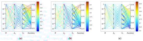
Figure 1. Overall accuracy versus the parameters $\alpha ,$ ${\lambda }_1,$ and ${\lambda }_2$ on the three datasets of SKLSPP. (a) Indian Pines dataset. (b) University of Pavia dataset. (c) Salinas dataset.

Figure 2 illustrates the changes in OA corresponding to the retained number of dimensions (2, 4, 6, 8, 10, 12, 14, 16, 18, 20, 22, 24, 26, 28, and 30). For comparison, the classification results of the original image and the PCA, NPE, LPP, LDA, KLDA, LRCRP, MFS-PE, and SKLSPP dimension-reduced results were also generated. Across all methods and datasets, the classification accuracy stabilizes when the number of dimensions exceeds a certain threshold. Therefore, 14, 12, and 12 dimensions are reasonable values for the proposed SKLSPP methods for the three datasets in subsequent classifications. In particular, since the rank of the between-class scatter matrix is $C-1$ (where $C$ is the number of classes), the dimensionality of LDA- and KDA-transformed data is up to $C-1$. Thus, the dimensionality of LDA and KDA is set to 15, 8, and 14 for the three test datasets. Finally, the extracted features from each method were used as input to a multiclass SVM classifier. A Gaussian kernel was employed for SVM, and the regularization and kernel parameters were optimized through cross-validation.

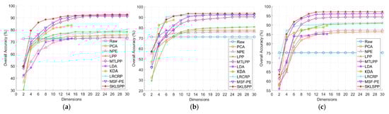
Figure 2. Classification accuracy versus reduced dimensionality of the three HSI datasets using different DR methods. (a) Indian Pines dataset. (b) University of Pavia dataset. (c) Salinas dataset.

4.3. Experimental Results

In this section, we systematically evaluate the proposed SKLSPP method through comparative experiments with classical DR methods and several state-of-the-art baselines on three hyperspectral datasets. The classification performance across the three benchmark datasets is presented in Table 1, Table 2 and Table 3. To ensure statistical reliability, each model was independently executed ten times on each dataset. Specifically, the tables delineate the individual mean class accuracy, average accuracy (AA), OA, and Kappa coefficient (κ) for the datasets, with accompanying standard deviations providing insights into the classification model’s robustness and performance consistency.

Table 1. Classification accuracy (%) for the Indian Pines dataset.

Class	RAW	PCA	NPE	LPP	MTLPP	LDA	KDA	LRCRP	MFS-PE	SKLSPP
	Mean ± Std	Mean ± Std	Mean ± Std	Mean ± Std	Mean ± Std	Mean ± Std	Mean ± Std	Mean ± Std	Mean ± Std	Mean ± Std
C1	24.04 ± 8.46	36.60 ± 11.81	34.19 ± 2.62	37.70 ± 7.88	92.44 ±2.38	31.70 ± 7.70	84.44 ± 0.12	96.12 ± 6.38	97.83 ± 1.30	99.26 ± 1.01
C2	62.60 ± 2.45	69.57 ± 3.01	71.55 ± 3.49	70.33 ± 1.33	87.24 ± 2.57	72.19 ± 2.20	63.96 ± 1.44	76.84 ± 3.13	82.31 ± 3.31	89.50 ± 5.64
C3	56.56 ± 5.52	63.94 ± 2.65	47.65 ± 0.91	69.46 ± 3.24	93.15 ± 4.13	55.99 ± 4.83	82.43 ± 1.61	79.37 ± 0.67	86.89 ± 1.41	91.13 ± 7.17
C4	31.93 ± 4.73	47.63 ± 5.63	31.97 ± 3.85	51.65 ± 6.83	92.43 ± 0.96	38.73 ± 4.06	86.80 ± 0.82	84.88 ± 2.68	99.54 ± 0.21	93.50 ± 0.60
C5	80.63 ± 6.54	85.80 ± 1.21	79.16 ± 1.68	87.44 ± 2.27	92.17 ± 1.83	83.96 ± 5.96	92.07 ± 0.51	89.02 ± 0.52	91.44 ± 0.75	96.08 ± 2.16
C6	89.18 ± 3.62	92.38 ± 2.04	95.33 ± 1.31	94.07 ± 1.69	99.28 ± 0.92	93.72 ± 3.66	95.22 ± 2.16	80.98 ± 4.56	99.88 ± 0.15	97.67 ± 0.99
C7	25.20 ± 18.76	50.83 ± 12.39	51.92 ± 2.44	61.30 ± 17.8	94.39 ± 0.18	46.60 ± 7.12	82.10 ± 2.91	63.42 ± 10.23	92.00 ± 3.06	99.23 ± 1.16
C8	94.37 ± 4.34	96.66 ± 1.79	92.88 ± 0.35	96.89 ± 1.69	98.15 ± 1.03	99.41 ± 0.40	98.19 ± 0.18	95.00 ± 1.60	100 ± 0	100 ± 0
C9	27.37 ± 8.52	20.00 ± 17.5	25.71 ± 1.48	35.55 ± 9.86	92.04 ± 0.91	49.72 ± 9.48	88.74 ± 1.94	56.53 ± 0.48	93.40 ± 1.27	86.00 ± 8.50
C10	62.22 ± 4.03	66.95 ± 2.59	60.28 ± 1.41	70.07 ± 2.74	89.24 ± 5.19	64.37 ± 1.03	77.10 ± 3.93	82.58 ± 4.27	93.06 ± 0.73	93.78 ± 2.93
C11	75.85 ± 2.48	78.26 ± 2.05	78.68 ± 0.32	81.10 ± 1.88	85.93 ± 2.32	75.14 ± 0.96	81.57 ± 4.32	84.60 ± 2.20	92.48 ± 0.25	95.45 ± 2.3
C12	54.78 ± 5.20	64.97 ± 4.83	53.95 ± 2.24	70.14 ± 2.33	93.09 ± 2.91	61.70 ± 2.98	82.98 ± 7.69	67.96 ± 0.69	94.38 ± 4.18	80.91 ± 7.3
C13	91.49 ± 4.49	94.74 ± 3.92	89.44 ± 6.74	97.37 ± 1.69	98.49 ± 1.43	95.24 ± 2.09	98.07 ± 0.26	94.23 ± 1.04	100 ± 0	98.96 ± 0.61
C14	93.54 ± 2.80	93.13 ± 2.21	94.86 ± 0.52	94.33 ± 1.14	95.74 ± 2.29	94.24 ± 1.74	99.00 ± 1.19	93.16 ± 1.23	98.42 ± 0.78	99.47 ± 0.72
C15	46.40 ± 4.65	50.00 ± 7.38	47.21 ± 2.73	57.85 ± 6.71	91.33 ± 1.52	57.70 ± 0.68	87.47 ± 2.51	78.67 ± 3.45	96.22 ± 3.32	89.94 ± 10.76
C16	51.10 ± 14.41	64.77 ± 8.03	67.79 ± 0.67	68.57 ± 7.08	99.41 ± 0.63	66.37 ± 5.44	81.80 ± 6.81	92.53 ± 0.11	92.63 ± 1.78	94.31 ± 3.12
AA	58.38 ± 4.63	66.51 ± 4.49	64.17 ± 1.83	70.30 ± 3.66	91.50 ± 0.72	69.11 ±1.07	83.87 ± 2.18	80.34 ± 2.39	93.04 ± 0.78	93.69 ± 1.48
OA	71.74 ± 1.06	76.25 ± 0.67	73.69 ± 0.2	78.96 ± 0.47	92.02 ± 0.64	74.06 ± 0.70	83.54 ± 1.39	80.67 ± 3.19	93.88 ± 0.58	94.54 ± 1.05
Kappa	67.64 ± 1.22	72.92 ± 0.82	70.63 ± 0.94	75.97 ± 0.54	91.28 ± 0.73	70.19 ± 0.82	81.40 ± 1.52	79.43 ± 2.17	92.65 ± 0.66	93.17 ± 1.21

Table 2. Classification accuracy (%) for the University of Pavia dataset.

Class	RAW	PCA	NPE	LPP	MTLPP	LDA	KDA	LRCRP	MFS-PE	SKLSPP
	Mean ± Std	Mean ± Std	Mean ± Std	Mean ± Std	Mean ± Std	Mean ± Std	Mean ± Std	Mean ± Std	Mean ± Std	Mean ± Std
C1	67.06 ± 2.79	68.87 ± 4.58	85.83 ± 1.76	78.63 ± 4.28	86.35 ± 1.44	86.99 ± 1.36	86.13 ± 2.00	95.25 ± 1.82	94.26 ± 1.07	89.04 ± 2.66
C2	76.33 ± 7.97	80.66 ± 1.10	75.97 ± 0.59	81.62 ± 3.05	91.97 ± 2.12	91.61 ± 1.20	82.09 ± 2.34	92.95 ± 2.10	93.20 ± 1.13	96.66 ± 0.52
C3	68.85 ± 9.73	72.30 ± 5.91	71.50 ± 5.52	81.10 ± 8.96	89.47 ± 2.3	77.87 ± 1.10	88.60 ± 0.45	75.68 ± 4.94	90.81 ± 1.50	91.65 ± 5.39
C4	73.32 ± 5.56	72.52 ± 6.83	75.89 ± 0.35	79.38 ± 5.94	88.53 ± 2.8	82.96 ± 5.45	91.70 ± 1.56	96.31 ± 0.76	92.33 ± 0.94	89.22 ± 5.41
C5	78.98 ± 0.04	89.83 ± 0.20	87.38 ± 1.15	96.39 ± 1.92	99.21 ± 1.03	87.25 ± 2.99	89.98 ± 0.03	90.07 ± 2.37	98.47 ± 0.21	99.64 ± 0.06
C6	64.34 ± 13.3	65.05 ± 10.52	65.16 ± 1.15	75.86 ± 4.99	91.17 ± 3.81	57.28 ± 7.75	92.42 ± 2.65	81.76 ± 3.21	93.01 ± 1.40	89.52 ± 6.28
C7	87.40 ± 2.56	87.02 ± 7.22	81.90 ± 8.31	90.64 ± 3.53	96.76 ± 0.44	78.64 ± 1.14	88.11 ± 4.23	88.01 ±3.32	99.83 ± 0.18	90.06 ± 0.25
C8	69.36 ± 9.18	69.23 ± 4.33	70.96 ± 1.02	72.23 ± 5.35	85.06 ± 1.65	66.25 ± 4.58	87.89 ± 1.42	70.11 ± 4.74	90.24 ± 1.18	95.07 ± 0.82
C9	93.11 ± 3.11	93.45 ± 4.33	85.36 ± 7.86	95.92 ± 1.76	98.17 ± 0.57	79.32 ± 6.60	89.73 ± 0.06	72.03 ± 3.10	95.27 ± 0.69	99.74 ± 0.26
AA	73.81 ± 4.70	77.18 ± 4.20	75.49 ± 0.47	81.25 ± 2.47	90.91 ± 0.92	78.64 ± 3.50	87.43 ± 0.60	86.47 ± 2.57	93.32 ± 1.03	93.40 ± 0.66
OA	71.75 ± 2.87	76.09 ± 1.47	76.03 ± 2.09	80.64 ± 1.85	90.56 ± 0.87	79.54 ± 1.77	87.05 ± 1.10	88.34 ± 2.76	93.74 ± 0.74	94.28± 0.04
Kappa	66.64 ± 3.18	69.30 ± 1.91	67.06 ± 0.73	75.20 ± 2.23	87.63 ± 1.08	77.41 ± 2.51	83.34 ± 1.33	83.88 ± 3.01	92.30 ± 0.85	92.49 ± 0.49

Table 3. Classification accuracy (%) for the Salinas dataset.

Class	RAW	PCA	NPE	LPP	MTLPP	LDA	KDA	LRCRP	MFS-PE	SKLSPP
	Mean ± Std	Mean ± Std	Mean ± Std	Mean ± Std	Mean ± Std	Mean ± Std	Mean ± Std	Mean ± Std	Mean ± Std	Mean ± Std
C1	96.79 ± 1.57	98.39 ± 3.49	99.27 ± 0.78	99.76 ± 0.27	100 ± 0	98.80 ± 0.65	99.15 ± 0.57	100 ± 0	100 ± 0	99.03 ± 1.06
C2	95.03 ± 3.92	98 ± 1.5	96.40 ± 2.82	99.11 ± 0.34	99.63 ± 0.23	94.63 ± 0.30	95.50 ± 0.10	98.85 ± 0.45	98.83 ± 0.29	99.91 ± 0.05
C3	83.91 ± 4.24	93.28 ± 5.46	87.07 ± 6.51	97.74 ± 1.86	98.22 ± 0.42	89.18 ± 4.73	83.96 ± 3.58	83.18 ± 2.19	93.48 ± 2.07	96.77 ± 1.92
C4	96.89 ± 1.46	97.93 ± 1.78	95.14 ± 0.37	98.48 ± 0.98	98.83 ± 0.47	89.16 ± 4.35	92.20 ± 1.57	89.17 ± 0.11	91.06 ± 1.16	99.88 ± 0.14
C5	89.66 ± 4.64	92.66 ± 1.88	97.98 ± 0.75	97.18 ± 1.13	96.99 ± 1.21	95.15 ± 0.80	96.43 ± 0.32	82.67 ± 3.02	99.23 ± 0.01	99.61 ± 0.13
C6	93.49 ± 4.92	96.81 ± 2.81	97.51 ± 0.31	98.91 ± 1.4	99.71 ± 0.27	96.59 ± 0.21	96.61 ± 2.39	99.56 ± 0.01	99.97 ± 0.17	99.71 ± 0.05
C7	94.21 ± 5.48	98.67 ± 0.32	99.11 ± 0.63	99.38 ± 0.45	92.16 ± 0.33	98.56 ± 0.24	97.66 ± 0.24	98.28 ± 0.47	100 ± 0	99.58 ± 0.02
C8	51.17 ± 13.11	66.34 ± 6.52	65.66 ± 8.25	75.39 ± 7.17	82.93 ± 3.47	74.77 ± 3.63	83.22 ± 2.63	87.01 ± 1.24	94.94 ± 1.60	98.38 ± 0.26
C9	92.95 ± 2.22	97.08 ± 2.04	96.36 ± 2.25	98.74 ± 0.6	99.24 ± 0.55	93.12 ± 0.47	93.97 ± 0.02	96.43 ± 0.70	94.07 ± 0.05	99.95 ± 0.04
C10	41.26 ± 11.49	79.22 ± 5.31	80.53 ± 7.79	87.80 ± 4.33	93.18 ± 1.73	90.87 ± 3.09	72.95 ± 4.57	85.67 ± 4.21	92.61 ± 2.68	94.89 ± 3.28
C11	85.70 ± 8.99	94.47 ± 2.59	94.97 ± 2.71	97.98 ± 0.39	98.54 ± 0.75	93.61 ± 1.23	91.39 ± 0.16	93.81 ± 1.60	92.82 ± 0.07	93.69 ± 7.96
C12	98.32 ± 1.74	96.21 ± 2.38	92.01 ± 1.58	98.91 ± 1.35	96.68 ± 0.14	90.10 ± 1.05	99.16 ± 0.12	93.73 ± 1.21	86.56 ± 0.99	99.82 ± 0.21
C13	96.47 ± 3.03	93.61 ± 2.64	94.09 ± 0.55	94.45 ± 1.73	95.39 ± 2.73	87.87 ± 5.73	90.98 ± 0.81	85.57 ± 0.97	97.56 ± 3.53	98.28 ± 0.54
C14	89.63 ± 3.09	90.19 ± 6.18	93.62 ± 2.79	96.71 ± 0.72	98.25 ± 0.98	90.01 ± 3.41	92.97 ± 0.32	97.11 ± 0.51	96.27 ± 1.02	95.88 ± 1.75
C15	61.50 ± 12.68	70.15 ± 12.93	72.18 ± 6.04	79.44 ± 3.11	82.59 ± 3.87	52.00 ± 5.19	66.69 ± 6.42	87.50 ± 2.07	95.93 ± 1.81	91.68 ± 5.95
C16	64.59 ± 5.13	88.11 ± 5.22	93.55 ± 3.99	97.27 ± 1.61	99.68 ± 0.25	96.42 ± 2.77	89.73 ± 3.04	95.20 ± 0.59	99.32 ± 2.59	99.50 ± 0.14
AA	79.33 ±2.87	87.19 ± 2.20	88.96 ± 1.06	90.27 ± 1.49	91.29 ± 0.91	89.55 ± 0.55	90.51 ± 3.56	91.26 ± 0.29	94.72 ± 0.48	97.51 ± 0.30
OA	77.20 ± 1	85.25 ± 1.84	85.03 ± 1.22	90.41 ± 1.67	93.55 ± 0.78	85.75 ± 0.27	89.24 ± 1.25	91.56 ± 0.37	95.21 ± 0.31	97.74 ± 0.61
Kappa	74.83 ± 1.07	83.63 ± 2.04	84.49 ± 1.36	89.35 ± 1.84	92.27 ± 0.87	84.12 ± 0.29	86.17 ± 1.91	90.56 ± 0.11	94.21 ± 0.48	97.48 ± 0.68

The proposed SKLSPP method achieved significantly improved classification performance compared to the existing DR techniques. On three test datasets, SKLSPP achieved overall accuracies of 94.54%, 94.28%, and 97.74% and Kappa coefficients of 93.17%, 92.49%, and 97.48%, respectively, representing substantial improvements over traditional methods. This superior performance was consistent across nearly all classes, with most achieving classification rates above 90%. Furthermore, previously challenging classes (e.g., C1 and C10 in the Indian Pines dataset) exhibited near-perfect classification rates. This enhancement is attributed to the novel local manifold learning strategy, which effectively captures intricate spatial–spectral relationships and overcomes limitations inherent in conventional DR approaches.

When compared to the baseline and classical methods, SKLSPP shows a significant performance gain. For instance, it substantially outperforms PCA and LDA by a large margin on all datasets, confirming the limitation of these linear techniques in handling complex spectral–spatial structures. Furthermore, against other strong non-linear or graph-based methods, such as KDA and LPP, SKLSPP consistently delivers better accuracy, highlighting the effectiveness of its novel structural constraints.

A detailed comparison with the best-performing existing techniques further validates the robustness of our approach. On the University of Pavia dataset, SKLSPP attains the highest AA of 93.40% and an OA of 94.28%, slightly edging out MFS-PE (OA: 93.74%) and notably outperforming LRCRP (OA: 88.34%) and MTLPP (OA:90.56). The advantage of SKLSPP is also evident at the class level across all datasets. It achieves perfect 100% accuracy in Class C8 of Indian Pines and Class C9 of University of Pavia and nears perfection in multiple Salinas classes (e.g., C2, C6, C7, C9, C12). While MFS-PE also shows remarkable class-wise performance, SKLSPP provides a more balanced and generalized solution, as evidenced by its superior OA and Kappa on complex scenes.

Figure 3, Figure 4 and Figure 5 present the classification maps produced by all considered methods on the test datasets, offering a more intuitive visualization of their performance. Visually, the proposed SKLSPP method yields significantly smoother homogeneous regions compared to other approaches. Notably, most of the classification errors highlighted by the rectangular boxes (Figure 3c–l, 4c–l, and 5c–l, respectively) are effectively corrected by SKLSPP. Furthermore, as observed in the area marked by the boxes in Figure 4i,l, both SKLSPP and the kernel-based KDA method achieve complete and accurate classification, successfully rectifying the misclassifications evident in other methods. This result underscores the advantage of kernel-based approaches in handling high-dimensional, non-linear hyperspectral data by mapping it into a more discriminative feature space. However, a more critical advantage of our method is revealed in more areas. While KDA exhibits significant classification noise and confusion among complex land cover types in this region, the proposed SKLSPP generates a markedly cleaner and more accurate map, closely resembling the ground truth. This superior performance can be attributed to the strategic integration of semantic label information directly into the sparse low-rank modeling process of SKLSPP. This design not only captures the non-linear data structure but also enhances the discriminative power of the resulting features by leveraging the supervisory signals from the training samples, thereby yielding more robust classification in complex scenarios.

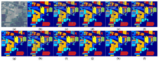
Figure 3. Classification maps for the Indian Pines dataset using different DR methods. (a) Hyperspectral image. (b) Ground truth. (c) Raw spectral. (d) PCA. (e) NPE. (f) LPP. (g) MTLPP. (h) LDA. (i) KDA. (j) LRCRP. (k) MFS-PE. (l) SKLSPP.

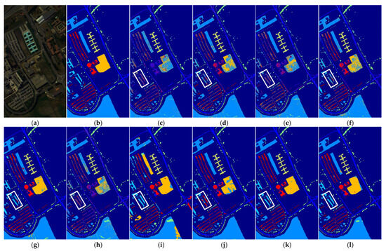
Figure 4. Classification maps for the University of Pavia dataset using different DR methods. (a) Hyperspectral image. (b) Ground truth. (c) Raw spectral. (d) PCA. (e) NPE. (f) LPP. (g) MTLPP. (h) LDA. (i) KDA. (j) LRCRP. (k) MFS-PE (l) SKLSPP.

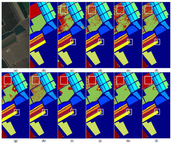
Figure 5. Classification maps for the Salinas dataset using different DR methods. (a) Hyperspectral image. (b) Ground truth. (c) Raw spectral. (d) PCA. (e) NPE. (f) LPP. (g) MTLPP. (h) LDA. (i) KDA. (j) LRCRP. (k) MFS-PE. (l) SKLSPP.

5. Conclusions

This study introduces the semantic-guided kernel low-rank sparse preserving projection (SKLSPP), a novel dimensionality reduction framework designed to overcome the limitations of conventional manifold learning methods in hyperspectral image analysis. By integrating semantic-aware kernel representation with spatially adaptive manifold regularization, SKLSPP effectively preserves the intrinsic geometric structure of high-dimensional data while enhancing discriminative feature extraction. Key innovations include a semantic guidance mechanism that integrates labels to explicitly preserve semantic consistency during feature transformation, a dynamically weighted graph Laplacian regularization term that captures both spectral similarity and spatial proximity among pixels, and a unified optimization framework that jointly learns the sparse codes, projection matrix, and manifold structure. These advancements address critical challenges in spectral redundancy, spatial incoherence, and noise sensitivity observed in previous approaches. Our experimental results across various real-world hyperspectral datasets demonstrate the superiority of SKLSPP, which outperformed comparison methods on the test datasets.

Despite these promising results, we recognize several avenues for future research. One important direction involves a more in-depth investigation into the robustness of SKLSPP against various types and levels of noise, which are commonly present in hyperspectral imagery. While the inherent low-rank and sparse properties of our model offer a degree of noise resilience, a dedicated analysis and potential further enhancement of the model’s robustness under more challenging noisy conditions would be beneficial for practical applications.

References

- Yu, W.B.; Zhang, M.; Huang, H.; Shen, Y.; Shen, G.X. Learning latent local manifold embeddings for hyperspectral feature extraction. J. Appl. Remote Sens. 2022, 16, 036513. [Google Scholar] [CrossRef]
- Liu, X.H.; Wang, T.M.; Wang, X.F. Joint Spectral-Spatial Representation Learning for Unsupervised Hyperspectral Image Clustering. Appl. Sci. 2025, 15, 8935. [Google Scholar] [CrossRef]
- Ghamisi, P.; Yokoya, N.; Li, J.; Liao, W.Z.; Liu, S.C.; Plaza, J.; Rasti, B.; Plaza, A. Advances in Hyperspectral Image and Signal Processing. IEEE Geosci. Remote Sens. Mag. 2017, 5, 37–78. [Google Scholar] [CrossRef]
- Kong, X.Y.; Zhao, Y.Q.; Chan, J.C.W.; Xue, J.Z. Hyperspectral Image Restoration via Spatial-Spectral Residual Total Variation Regularized Low-Rank Tensor Decomposition. Remote Sens. 2022, 14, 511. [Google Scholar] [CrossRef]
- Wu, L.; Huang, J.; Guo, M.S. Multidimensional Low-Rank Representation for Sparse Hyperspectral Unmixing. IEEE Geosci. Remote Sens. Lett. 2023, 20, 5502805. [Google Scholar] [CrossRef]
- de Morsier, F.; Borgeaud, M.; Gass, V.; Thiran, J.-P.; Tuia, D. Kernel Low-Rank and Sparse Graph for Unsupervised and Semi-Supervised Classification of Hyperspectral Images. IEEE Trans. Geosci. Remote Sens. 2016, 54, 3410–3420. [Google Scholar] [CrossRef]
- Geng, X.Y.; Guo, Q.; Hui, S.X.; Yang, M.; Zhang, C.M. Tensor robust PCA with nonconvex and nonlocal regularization. Comput. Vis. Image Underst. 2024, 243, 104007. [Google Scholar] [CrossRef]
- Reidl, J.; Starke, J.; Omer, D.B.; Grinvald, A.; Spors, H. Independent component analysis of high-resolution imaging data identifies distinct functional domains. Neuroimage 2007, 34, 94–108. [Google Scholar] [CrossRef]
- Wang, Q.; Meng, Z.T.; Li, X.L. Locality Adaptive Discriminant Analysis for Spectral-Spatial Classification of Hyperspectral Images. IEEE Geosci. Remote Sens. Lett. 2017, 14, 2077–2081. [Google Scholar] [CrossRef]
- Huang, K.K.; Dai, D.Q.; Ren, C.X.; Lai, Z.R. Learning Kernel Extended Dictionary for Face Recognition. IEEE Trans. Neural Netw. Learn. Syst. 2017, 28, 1082–1094. [Google Scholar] [CrossRef]
- Belkin, M.; Niyogi, P. Laplacian Eigenmaps for Dimensionality Reduction and Data Representation. Neural. Comput. 2003, 15, 1373–1396. [Google Scholar] [CrossRef]
- He, X.; Cai, D.; Yan, S.; Zhang, H.J. Neighborhood Preserving Embedding. In Proceedings of the Tenth IEEE International Conference on Computer Vision, Beijing, China, 17–21 October 2005. [Google Scholar]
- Zhang, T.H.; Tao, D.C.; Li, X.L.; Yang, J. Patch Alignment for Dimensionality Reduction. IEEE Trans. Knowl. Data Eng. 2009, 21, 1299–1313. [Google Scholar] [CrossRef]
- Zheng, D.; Du, X.; Cui, L. Tensor Locality Preserving Projections for Face Recognition. In Proceedings of the IEEE International Conference on Systems Man & Cybernetics, Istanbul, Turkey, 10–13 October 2010; pp. 2347–2350. [Google Scholar]
- Sugiyama, M. Dimensionality reduction of multimodal labeled data by local fisher discriminant analysis. J. Mach. Learn. Res. 2007, 8, 1027–1061. [Google Scholar]
- Yan, S.C.; Xu, D.; Zhang, B.Y.; Zhang, H.J.; Yang, Q.; Lin, S. Graph embedding and extensions: A general framework for dimensionality reduction. IEEE Trans. Pattern Anal. Mach. Intell. 2007, 29, 40–51. [Google Scholar] [CrossRef]
- Cheng, B.; Yang, J.C.; Yan, S.C.; Fu, Y.; Huang, T.S. Learning With l1-Graph for Image Analysis. IEEE Trans. Image Process. 2010, 19, 858–866. [Google Scholar] [CrossRef]
- Ly, N.H.; Du, Q.; Fowler, J.E. Sparse Graph-Based Discriminant Analysis for Hyperspectral Imagery. IEEE Trans. Geosci. Remote Sens. 2014, 52, 3872–3884. [Google Scholar] [CrossRef]
- Candès, E.; Recht, B. Exact Matrix Completion via Convex Optimization. Commun. ACM 2012, 55, 111–119. [Google Scholar] [CrossRef]
- Liu, G.C.; Lin, Z.C.; Yan, S.C.; Sun, J.; Yu, Y.; Ma, Y. Robust Recovery of Subspace Structures by Low-Rank Representation. IEEE Trans. Pattern Anal. Mach. Intell. 2013, 35, 171–184. [Google Scholar] [CrossRef]
- Liu, Y.F.; Chen, J.H.; Li, Y.Q.; Wu, T.S.; Wen, H. Joint face normalization and representation learning for face recognition. Pattern. Anal. Appl. 2024, 27, 64. [Google Scholar] [CrossRef]
- Baiju, P.S.; Jayan, P.D.; George, S.N. Tensor total variation regularised low-rank approximation framework for video deraining. Iet Image Process 2020, 14, 3602–3612. [Google Scholar] [CrossRef]
- Yan, W.Z.; Yang, M.; Li, Y.M. Robust Low Rank and Sparse Representation for Multiple Kernel Dimensionality Reduction. IEEE Trans. Circuits Syst. Video Technol. 2023, 33, 1–15. [Google Scholar] [CrossRef]
- Zhang, Z.; Xu, Y.; Shao, L.; Yang, J. Discriminative Block-Diagonal Representation Learning for Image Recognition. IEEE Trans. Neural Netw. Learn. Syst. 2018, 29, 3111–3125. [Google Scholar] [CrossRef]
- Wong, W.K.; Lai, Z.H.; Wen, J.J.; Fang, X.Z.; Lu, Y.W. Low-Rank Embedding for Robust Image Feature Extraction. IEEE Trans. Image Process. 2017, 26, 2905–2917. [Google Scholar] [CrossRef] [PubMed]
- Chen, J.; Mao, H.; Sang, Y.S.; Yi, Z. Subspace clustering using a symmetric low-rank representation. Knowl. Based Syst. 2017, 127, 46–57. [Google Scholar] [CrossRef]
- Du, H.S.; Wang, Y.X.; Zhang, F.; Zhou, Y. Low-Rank Discriminative Adaptive Graph Preserving Subspace Learning. Neural Process. Lett. 2020, 52, 2127–2149. [Google Scholar] [CrossRef]
- Jiang, X.W.; Xiong, L.W.; Yan, Q.; Zhang, Y.S.; Liu, X.B.; Cai, Z.H. Unsupervised Dimensionality Reduction for Hyperspectral Imagery via Laplacian Regularized Collaborative Representation Projection. IEEE Geosci. Remote Sens. Lett. 2022, 19, 6007805. [Google Scholar] [CrossRef]
- Xie, L.F.; Yin, M.; Yin, X.Y.; Liu, Y.; Yin, G.F. Low-Rank Sparse Preserving Projections for Dimensionality Reduction. IEEE Trans. Image Process. 2018, 27, 5261–5274. [Google Scholar] [CrossRef]
- Teng, L.Y.; Tang, F.Y.; Zheng, Z.F.; Kang, P.P.; Teng, S.H. Kernel-Based Sparse Representation Learning With Global and Local Low-Rank Label Constraint. IEEE Trans. Comput. Soc. Syst. 2024, 11, 488–502. [Google Scholar] [CrossRef]
- Deng, Y.-J.; Li, H.-C.; Pan, L.; Shao, L.-Y.; Du, Q.; Emery, W.J. Modified Tensor Locality Preserving Projection for Dimensionality Reduction of Hyperspectral Images. IEEE Geosci. Remote Sens. Lett. 2018, 15, 277–281. [Google Scholar] [CrossRef]
- Chen, K.; Yang, G.G.; Wang, J.; Du, Q.; Su, H.J. Unsupervised Dimensionality Reduction With Multifeature Structure Joint Preserving Embedding for Hyperspectral Imagery. IEEE J. Sel. Top. Appl. Earth Obs. Remote Sens. 2023, 16, 7585–7599. [Google Scholar] [CrossRef]
Disclaimer/Publisher’s Note: The statements, opinions and data contained in all publications are solely those of the individual author(s) and contributor(s) and not of MDPI and/or the editor(s). MDPI and/or the editor(s) disclaim responsibility for any injury to people or property resulting from any ideas, methods, instructions or products referred to in the content. |
© 2026 by the authors. Licensee MDPI, Basel, Switzerland. This article is an open access article distributed under the terms and conditions of the Creative Commons Attribution (CC BY) license.