Traffic Flow Prediction Model Based on Attention Mechanism Spatio-Temporal Graph Convolutional Network on U.S. Highways

Abstract

Traffic flow prediction is a fundamental component of intelligent transportation systems and plays a critical role in traffic management and autonomous driving. However, accurately modeling highway traffic remains challenging due to dynamic congestion propagation, lane-level heterogeneity, and non-recurrent traffic events. To address these challenges, this paper proposes an improved attention-mechanism spatio-temporal graph convolutional network, termed AMSGCN, for highway traffic flow prediction. AMSGCN introduces an adaptive adjacency matrix learning mechanism to overcome the limitations of static graphs and capture time-varying spatial correlations and congestion propagation paths. A hierarchical multi-scale spatial attention mechanism is further designed to jointly model local congestion diffusion and long-range bottleneck effects, enabling an adaptive spatial receptive field under congested conditions. To enhance temporal modeling, a gating-based fusion strategy dynamically balances periodic patterns and recent observations, allowing effective prediction under both regular and abnormal traffic scenarios. In addition, direction-aware encoding is incorporated to suppress interference from opposite-direction lanes, which is essential for directional highway traffic systems. Extensive experiments on multiple benchmark datasets, including PeMS and PEMSF, demonstrate the effectiveness and robustness of AMSGCN. In particular, on the I-24 MOTION dataset, AMSGCN achieves an RMSE reduction of 11.0% compared to ASTGCN and 17.4% relative to the strongest STGCN baseline. Ablation studies further confirm that dynamic and multi-scale spatial attention provides the primary performance gains, while temporal gating and direction-aware modeling offer complementary improvements. These results indicate that AMSGCN is a robust and effective solution for highway traffic flow prediction.

1. Introduction

With the rapid advancement of sensing technologies, modern Intelligent Transportation Systems (ITS) increasingly rely on heterogeneous traffic sensors to continuously monitor traffic states across large-scale road networks. These sensing infrastructures, including loop detectors, roadside cameras, and trajectory-based monitoring systems, enable the collection of fine-grained traffic variables such as speed, flow, and occupancy. Leveraging historical traffic observations together with road network topology, traffic forecasting aims to predict future traffic dynamics, which plays a critical role in congestion mitigation, traffic management, and route guidance [1].

Accurate traffic flow prediction has undergone a significant paradigm shift, evolving from classical statistical time-series analysis to sophisticated data-driven machine learning and deep learning models. This evolution is driven by the increasing availability of large-scale traffic data from sensors, GPS, and IoT devices, coupled with advancements in computational power. Early models, while theoretically sound, often failed to capture the complex, non-linear, and dynamic spatiotemporal dependencies inherent in traffic networks. Contemporary research is characterized by a dominant trend towards hybrid intelligent frameworks that synergistically combine the strengths of different methodologies to overcome individual limitations [1,2]. This comprehensive review synthesizes current research, highlighting key methodological strands—from foundational models to cutting-edge deep learning architectures and emerging paradigms—and outlines persistent challenges and promising future trajectories.

Traditional statistical approaches, most notably the Autoregressive Integrated Moving Average (ARIMA) model and its variants (e.g., SARIMA), have served as foundational benchmarks in traffic forecasting [3]. Their strength lies in modeling linear relationships within stationary time-series data, offering simplicity, interpretability, and computational efficiency. The Kalman filter, another classical tool, is effective for real-time estimation and short-term prediction within state-space models. However, the core limitation of these models is their inherent assumption of linearity and stationarity. Traffic flow is a dynamic process influenced by complex, non-linear interactions across space and time, as well as external factors like weather, incidents, and social events. Consequently, pure statistical models often exhibit poor performance in capturing sudden fluctuations, long-term dependencies, and the intricate patterns present in large-scale urban networks [4]. Their primary value in contemporary research is often as a component in hybrid models or as a baseline for comparing more complex approaches.Recent studies have further explored the potential of machine learning approaches for traffic prediction [5], and comprehensive surveys have been conducted on LSTM-based forecasting methods [6].

The limitations of traditional models catalyzed the adoption of machine learning (ML). Shallow models like Support Vector Regression (SVR) and Random Forests demonstrated an improved capacity to model non-linearities. However, the true revolution began with the application of deep learning, particularly Recurrent Neural Networks (RNNs) and their advanced variants, Long Short-Term Memory (LSTM) and Gated Recurrent Unit (GRU) networks [4,7]. These architectures are inherently designed to handle sequential data, making them exceptionally suitable for learning temporal dependencies in traffic flow. They can “remember” information from previous time steps, allowing them to model patterns over varying horizons more effectively than statistical methods. This capability made LSTM and GRU the de facto standard for temporal modeling in traffic prediction for several years, setting a new performance benchmark and forming the temporal backbone of many subsequent hybrid and spatial–temporal models.

A major breakthrough came with the explicit modeling of spatial dependencies. Traffic networks are naturally represented as graphs, where intersections are nodes and road segments are edges. This insight led to the adoption of Graph Neural Networks (GNNs), especially Graph Convolutional Networks (GCNs) and their spatiotemporal extensions. Models like the Spatiotemporal Graph Convolutional Network (STGCN) integrate graph convolutions to capture spatial features from the road network and temporal convolutions (or RNNs) to capture dynamic patterns, achieving superior performance by jointly modeling both dimensions [8]. This paradigm has since been extensively refined. For instance, causality graphs have been used to model the dynamic influence between airports in a multi-airport system, moving beyond simple physical proximity to functional relationships [9]. Recent innovations include multi-task spatiotemporal networks for highway traffic flow prediction [10], contrastive learning-based adaptive graph augmentation methods [11], and graph embedding-based convolutional recurrent attention networks [12], further enriching the methodological landscape of spatio-temporal graph modeling.Recent innovations focus on dynamic graph structures. The Attention-based Dynamic GCN (ADGCN) and the Spatiotemporal Interactive Learning Dynamic Adaptive GCN (SILDAGCN) learn dynamic adjacency matrices in real-time, allowing the model to adapt to changing traffic conditions and uncover latent spatial relationships that fixed graphs might miss. Furthermore, the Hybrid Spatiotemporal GNN (HSTGNN) attempts to fuse multiple types of spatial dependencies—static (network topology), dynamic (real-time traffic), and semantic (similar functional roles)—alongside multi-scale temporal attention for a more comprehensive representation [13].

The current state-of-the-art is dominated by hybrid models that combine methodologies to leverage their complementary strengths. A common strategy is fusing classical statistical models with deep learning. For example, ARIMA can be used to extract and forecast linear components of the series, while a deep learning model (like Conv-LSTM) concurrently learns the non-linear residuals, leading to more robust predictions. This principle extends beyond time-series; a multivariate hybrid framework using Multivariate Empirical Mode Decomposition (MEMD) for noise reduction before applying tree-based models has shown significant accuracy gains. Another critical innovation is the pervasive integration of attention mechanisms. Inspired by Transformer architectures, attention allows models to selectively focus on the most relevant information from the input sequence, both temporally and spatially. The Confined Attention Mechanism within a Bi-GRU model enhances focus on critical time steps for more precise predictions [14]. Attention is now a core component in advanced GNNs, as seen in ADGCN and HSTGNN, enabling them to weigh the importance of different node connections dynamically.

Real-world deployment requires models that are robust to practical issues. Research has actively addressed missing data and multiple influencing factors (weather, holidays, events) through specialized model designs that incorporate data imputation techniques and multi-source data fusion [15]. Ensemble methods, which combine predictions from multiple base learners (e.g., different ML models), are employed to reduce variance and improve overall stability and accuracy [16]. Emerging technologies are also being integrated. Blockchain has been proposed within an SVD-ARIMA framework for IIoT environments to ensure data security and trustworthiness [17]. Generative Adversarial Networks (GANs) are gaining traction for their ability to generate realistic traffic data, impute missing values, and even perform prediction by learning the underlying data distribution, offering a powerful tool for enhancing robustness, especially in data-scarce or highly stochastic scenarios. Furthermore, improved deep learning models utilizing wavelet transforms have been employed to enhance prediction performance [18], and physics-informed deep learning embeds domain knowledge into the model’s architecture or loss function to improve generalizability and interpretability [19,20]. Despite these advances, existing traffic forecasting models still exhibit notable limitations in modeling spatio-temporal dynamics, especially at the lane level and under complex traffic conditions [21]. Inspired by Transformer architectures, attention enables models to dynamically focus on the most relevant temporal segments and spatial neighbors. Chauhan et al. [14] proposed a confined attention mechanism driven Bi-GRU model, which restricts attention to the most informative spatio-temporal dependencies, improving both accuracy and efficiency.

In parallel, interpretability has emerged as an increasingly important research direction. While tree-based models combined with SHAP analysis, such as XGB+SHAP, have been widely used to provide policy-oriented insights [22], recent work has explored explainability within deep learning frameworks. Guo et al. [23] proposed an explainable traffic flow prediction framework based on large language models, capable of generating human-understandable explanations alongside numerical forecasts. These studies highlight a growing demand for models that not only achieve high accuracy but also offer meaningful interpretations of traffic dynamics. Recent studies have further expanded traffic forecasting by incorporating heterogeneous data sources and alternative learning paradigms. Wang et al. [24] demonstrated that fusing visually quantified features, such as vehicle density and composition extracted from traffic videos, can significantly enhance heterogeneous traffic flow prediction. Méndez et al. [25] proposed a hybrid CNN-BiLSTM framework for long-term traffic flow forecasting, leveraging CNNs for spatial feature extraction and BiLSTMs for bidirectional temporal dependency modeling. In resource-constrained environments, Ali et al. [26] developed a resource-aware multi-graph neural network tailored for multi-access edge computing systems, emphasizing efficiency and scalability for urban traffic prediction.

To address these challenges, we propose a dynamic spatio-temporal traffic forecasting framework that explicitly models time-varying spatial relationships, multi-scale spatial dependencies, and adaptive temporal fusion. The proposed model consists of three tightly coupled modules:

1.

Dynamic Relationship Graph Learning, which constructs time-dependent graphs to capture high-order and evolving interactions among lane-level nodes.

2.

Multi-Scale Spatial Attention Learning, which models spatial dependencies at local, lane-level, and global scales, and adaptively fuses them through cross-scale attention.

3.

Gating-based Temporal Fusion, which adaptively balances short-term and long-term temporal representations by modulating their contributions using a learnable gating mechanism.

Different from policy-oriented models such as XGB + SHAP [22], our work focuses on integrating these components into a unified framework to effectively capture complex traffic dynamics across multiple spatial and temporal resolutions, leading to improved prediction robustness and interpretability.

2. Problem Definition

2.1. Traffic Network Definition

To handle non-Euclidean spatial data, this paper first formalizes the physical traffic network as a graph structure. In this graph, each node corresponds to a traffic sensor and edges represent the spatial connectivity between nodes. This abstraction is used for applying graph convolution operations to capture spatial dependencies. The traffic network is defined as an undirected graph $\mathcal{G}=(\mathcal{V},\mathcal{E},\mathrm{A})$, where $\mathcal{V}$ is the set of nodes, $\left|\mathcal{V}\right|=\mathrm{N}$ represents the number of detectors in the network; $\mathcal{E}$ is the set of edges, representing the connection relationships between nodes; $\mathrm{A}\in {\mathbb{R}}^{\mathrm{N}\times \mathrm{N}}$ is the adjacency matrix. Each node detects $\mathrm{F}$ traffic measurements (such as flow, speed, occupancy and vehicle lane change rate) at each time slice with the same sampling frequency.

2.2. Traffic Flow Prediction Problem

The traffic flow prediction task can be formalized as a typical spatio-temporal sequence prediction problem. Its core objective is: given the historical observation sequence of the entire sensor network over a continuous period, learn a mapping function to predict the traffic state of all nodes for a future period.

Let ${\mathrm{x}}_{\mathrm{t}}^{\mathrm{i}}\in {\mathbb{R}}^{\mathrm{F}}$ represents all feature values of node $i$ at time $\mathrm{t}$, and ${\mathrm{X}}_{\mathrm{t}}=({\mathrm{x}}_{\mathrm{t}}^1,{\mathrm{x}}_{\mathrm{t}}^2,\dots ,{\mathrm{x}}_{\mathrm{t}}^{\mathrm{N}}{)}^{\mathrm{T}}\in {\mathbb{R}}^{\mathrm{N}\times \mathrm{F}}$ represent the feature matrix of all nodes at time $\mathrm{t}$.

The historical observation sequence is represented as:

$$\mathrm{X}=({\mathrm{X}}_1,{\mathrm{X}}_2,\dots ,{\mathrm{X}}_{\mathsf{\tau }}{)}^{\mathrm{T}}\in {\mathbb{R}}^{\mathrm{N}\times \mathrm{F}\times \mathsf{\tau }},$$

(1)

Prediction Target: Given the historical observations $\mathrm{X}$ of $\mathsf{\tau }$ time slices, predict the traffic flow for the future ${\mathrm{T}}_{\mathrm{p}}$ time slices:

$$\mathrm{Y}=({\mathrm{y}}^1,{\mathrm{y}}^2,\dots ,{\mathrm{y}}^{\mathrm{N}}{)}^{\mathrm{T}}\in {\mathbb{R}}^{\mathrm{N}\times {\mathrm{T}}_{\mathrm{p}}},$$

(2)

where ${\mathrm{y}}^{\mathrm{i}}=({\mathrm{y}}_{\mathsf{\tau }+1}^{\mathrm{i}},{\mathrm{y}}_{\mathsf{\tau }+2}^{\mathrm{i}},\dots ,{\mathrm{y}}_{\mathsf{\tau }+{\mathrm{T}}_{\mathrm{p}}}^{\mathrm{i}})\in {\mathbb{R}}^{{\mathrm{T}}_{\mathrm{p}}}$ is the future traffic flow sequence for node $\mathrm{i}$.

We aim to construct a function f(·) that maps the historical time series over $\mathsf{\tau }$ timesteps to predict the subsequent ${\mathrm{T}}_{\mathrm{p}}$ time steps:

$$\mathrm{f}({\mathrm{X}}_1,{\mathrm{X}}_2,\dots ,{\mathrm{X}}_{\mathsf{\tau }}{)}^{\mathrm{T}}\to ({\mathrm{y}}^1,{\mathrm{y}}^2,\dots ,{\mathrm{y}}^{\mathrm{N}}{)}^{\mathrm{T}}$$

(3)

3. Model Methodology

3.1. Overall Model Architecture

The design objective of the proposed AMSGCN is to comprehensively model the complex and dynamic spatio-temporal regularities of traffic flow in highway scenarios, rather than relying on fixed and predefined temporal partitions. As illustrated in Figure 1, AMSGCN adopts a unified spatio-temporal modeling framework that explicitly accounts for time-varying spatial interactions, multi-scale spatial dependencies, directional propagation, and adaptive temporal fusion.

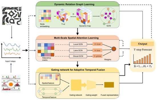
Figure 1. The overall architecture of the proposed AMSGCN model.

Instead of processing historical data through independent branches, AMSGCN integrates information from different temporal scales in a more flexible and data-driven manner. The model employs a dynamic relationship graph learning module to adaptively capture time-dependent spatial correlations among traffic nodes. To further characterize heterogeneous spatial interactions, a multi-scale spatial attention mechanism is introduced to simultaneously model local congestion effects and long-range bottleneck influences. To address the varying importance of short-term fluctuations, AMSGCN incorporates a gated temporal fusion module, which dynamically balances short-term and long-term temporal features based on traffic dynamics.

These components are jointly embedded within stacked spatio-temporal convolutional blocks. Finally, the learned spatio-temporal representations are aggregated to produce traffic flow predictions. This unified design allows AMSGCN to flexibly adapt to different traffic regimes while maintaining robustness across multiple predictions.

3.2. Module1: Dynamic Relationship Graph Learning with Direction-Aware Graph Convolution

Let $X_t\in {\mathbb{R}}^{N\times F}$ denote the node-feature matrix at time step $t$, where $N$ is the number of traffic nodes and $F$ is the feature dimension. To move beyond static distance-based connectivity, we learn a time-dependent adjacency tensor $A\in {\mathbb{R}}^{N_t\times N\times F}$ that captures high-order and time-varying relationships among nodes.

Following the tensor-factorization idea, we define: time-slot embedding: $E^{\left(t\right)}\in {\mathbb{R}}^{N_t\times d}$, source (starting) node embedding: $E^{\left(s\right)}\in {\mathbb{R}}^{N\times d}$, target (ending) node embedding: $E^{\left(e\right)}\in {\mathbb{R}}^{N\times d}$ and core tensor: $K\in {\mathbb{R}}^{d\times d\times d}$.

At each time slot $t$, and node pair $(i, j)$, we compute the unnormalized affinity:

$$A_{t,i,j}^{\prime }=\sum _{o=1}^d\sum _{q=1}^d\sum _{r=1}^d{K}_{o,q,r}{E}_{t,o}^{\left(t\right)}{E}_{i,q}^{\left(e\right)}{E}_{j,r}^{\left(s\right)},$$

(4)

We then apply a nonlinearity and row-wise softmax to obtain a valid adjacency (each row sums to 1):

$$\begin{gathered} A_{t,i,j}^{″}=max(0, A_{t,i,j}^{\prime }), \\ {A}_{t,i,j}={\displaystyle \frac{exp\left(A_{t,i,j}^{″}\right)}{\sum _{n=1}^{N}exp\left(A_{t,i,n}^{″}\right)}}. \end{gathered}$$

(5)

Let $H^{\left(0\right)}\in X_t$. We first normalize adjacency using row degree $D_t$:

$$D_t(i,i)=\sum _{j=1}^N{A}_{t,i,j},\hspace{1em}{\tilde{A}}_t=D_t^{-1}{A}_t.$$

(6)

A standard one-hop dynamic graph convolution is defined in (4) where $H_t^{\left(l\right)}\in {\mathbb{R}}^{N\times F_l}$, $W^{\left(l\right)}\in {\mathbb{R}}^{F_l\times F_{l+1}}$, and $\sigma (·)$ is a nonlinearity.

$$H_t^{(l+1)}=\sigma \left({\tilde{A}}_t,H_t^{\left(l\right)},W^{\left(l\right)}\right),$$

(7)

To explicitly model multi-hop which means local and farther bottleneck influence, we can write the aggregated output at time (t) as (5) where $W_k\in {\mathbb{R}}^{F\times F^{\prime }}$ and $H_t^{sp}\in {\mathbb{R}}^{N\times F^{\prime }}$.

$$H_t^{\mathrm{sp}}=\sum _{k=0}^K{\tilde{A}}_t^{,k},X_t,W_k,$$

(8)

Highway traffic influence is directional where upstream conditions propagate downstream, while severe congestion may exhibit feedback patterns. Therefore, we extend the dynamic graph convolution to be direction-aware by separately modeling forward and backward propagation. Define forward and backward normalized adjacencies:

$$\begin{gathered} {\tilde{A}}_t^{\to }=D_t^{-1}{A}_t,\hspace{1em}\hspace{1em} \\ {\tilde{A}}_t^{\leftarrow }=(D_t^{\top }{)}^{-1}{A}_t^{\top }. \end{gathered}$$

(9)

Based on the forward/backward multi-hop aggregations, we fuse them with an adaptive gate ${\mathsf{\lambda }}_{\mathrm{t}}\in (0,1)$:

$$\begin{gathered} H_t^{\to }=\sum _{k=0}^K{\left({\tilde{A}}_t^{\to }\right)}^k{X}_t{W}_k^{\to }, \\ {H}_t^{\leftarrow }=\sum _{k=0}^K{\left({\tilde{A}}_t^{\leftarrow }\right)}^k{X}_t{W}_k^{\leftarrow }. \\ {H}_t^{\mathrm{out}}={\lambda }_t{H}_t^{\to }+(1-{\lambda }_t)H_t^{\leftarrow }. \end{gathered}$$

(10)

3.3. Module2: Multi-Scale Spatial Attention Learning

Traffic congestion propagation exhibits distinct spatial patterns at different scales, including short-range car-following interactions, lane-level coupling, and long-range congestion waves. To capture such heterogeneous spatial dependencies, we introduce a multi-scale spatial attention module that operates on the dynamic relationship graph learned in Module1. Let $H_t\in {\mathbb{R}}^{N\times D}$ denote the node representations at time step $t$, $A_t\in {\mathbb{R}}^{\mathrm{N}\times \mathrm{N}}$ denote the learned dynamic adjacency matrix at time $\mathrm{t}$. Based on the strength of dynamic interactions, we construct three scale-specific adjacency matrices from ${\mathrm{A}}_{\mathrm{t}}$ to model spatial dependencies.

First is local-scale graph (strong interactions). This graph captures short-range car-following behavior and immediate spatial influence between adjacent road nodes:

$$A_t^{\left(l\right)}(i,j)=\left\{\begin{array}{ll}{A}_t(i,j),& A_t(i,j)\ge {\theta }_{\mathrm{high}}\\ 0,& \mathrm{otherwise}\end{array}\right.$$

(11)

where ${\mathsf{\theta }}_{\mathrm{h}\mathrm{i}\mathrm{g}\mathrm{h}}$ is a predefined high threshold to filter strong local interactions (e.g., ${\mathsf{\theta }}_{\mathrm{h}\mathrm{i}\mathrm{g}\mathrm{h}}=0.7$). Second is lane-scale graph (lane-level interactions). This graph models interactions within the same lane and adjacent lanes, which is critical for capturing lane-specific congestion spillover:

$$A_t^{\left(m\right)}=A_t\odot M_{\mathrm{lane}}$$

(12)

where ${\mathrm{M}}_{\mathrm{lane}}\in \{\mathrm{0,1}{\}}^{\mathrm{N}\times \mathrm{N}}$ is a predefined lane connectivity mask (1 indicates nodes in the same/adjacent lanes, 0 otherwise). Third is global-scale graph (long-range interactions). This graph captures long-range congestion propagation like congestion waves spreading across multiple road segments:

$$A_t^{\left(g\right)}(i,j)=\left\{\begin{array}{ll}{A}_t(i,j),& A_t(i,j)\ge {\theta }_{\mathrm{low}}\\ 0,& \mathrm{otherwise}\end{array}\right.$$

(13)

where ${\mathsf{\theta }}_{\mathrm{low}}$ is a low threshold (e.g.,${\mathsf{\theta }}_{\mathrm{low}}=0.2$) to retain weak but meaningful long-range interactions. Each adjacency matrix (${\mathrm{A}}_{\mathrm{t}}^{\left(\mathrm{l}\right)}$, ${\mathrm{A}}_{\mathrm{t}}^{\left(\mathrm{m}\right)}$, ${\mathrm{A}}_{\mathrm{t}}^{\left(\mathrm{g}\right)}$) is row-normalized to ensure numerical stability during graph convolution and attention aggregation.

For each spatial scale $s\in \{l,m,g\}$, we compute scale-specific node representations using graph-based attention aggregation, which integrates structural constraints from scale-specific adjacency matrices with data-driven attention scores. We project the original node features into query, key, and value spaces for each scale:

$${\mathrm{Q}}_{\mathrm{t}}^{\left(\mathrm{s}\right)}={\mathrm{H}}_{\mathrm{t}}{\mathrm{W}}_{\mathrm{Q}}^{\left(\mathrm{s}\right)},\hspace{1em}{\mathrm{K}}_{\mathrm{t}}^{\left(\mathrm{s}\right)}={\mathrm{H}}_{\mathrm{t}}{\mathrm{W}}_{\mathrm{K}}^{\left(\mathrm{s}\right)},\hspace{1em}{\mathrm{V}}_{\mathrm{t}}^{\left(\mathrm{s}\right)}={\mathrm{H}}_{\mathrm{t}}{\mathrm{W}}_{\mathrm{V}}^{\left(\mathrm{s}\right)}$$

(14)

where ${\mathrm{W}}_{\mathrm{Q}}^{\left(\mathrm{s}\right)},{\mathrm{W}}_{\mathrm{K}}^{\left(\mathrm{s}\right)},{\mathrm{W}}_{\mathrm{V}}^{\left(\mathrm{s}\right)}\in {\mathbb{R}}^{\mathrm{D}\times \mathrm{D}}$ are learnable scale-specific projection matrices, and $\mathrm{D}$ is the dimension of node features. The raw attention scores between nodes are computed as scaled dot-product attention to avoid gradient vanishing:

$${\mathrm{S}}_{\mathrm{t}}^{\left(\mathrm{s}\right)}={\displaystyle \frac{{\mathrm{Q}}_{\mathrm{t}}^{\left(\mathrm{s}\right)}{{\mathrm{K}}_{\mathrm{t}}^{\left(\mathrm{s}\right)}}^{\mathrm{\top }}}{\sqrt{\mathrm{D}}}}$$

(15)

To enforce spatial consistency with the scale-specific graph structure, we mask the attention scores using the adjacency matrix. This ensures that attention is only computed between nodes with physical interactions at the target scale. We normalize the masked attention scores using softmax to obtain valid attention weights:

$$\begin{gathered} {\tilde{\mathrm{S}}}_{\mathrm{t}}^{\left(\mathrm{s}\right)}={\mathrm{S}}_{\mathrm{t}}^{\left(\mathrm{s}\right)}\odot {\mathrm{A}}_{\mathrm{t}}^{\left(\mathrm{s}\right)} \\ {\mathsf{\alpha }}_{\mathrm{t}}^{\left(\mathrm{s}\right)}=\mathrm{softmax}\left({\tilde{\mathrm{S}}}_{\mathrm{t}}^{\left(\mathrm{s}\right)}\right) \end{gathered}$$

(16)

Finally, the scale-specific node representations are obtained by aggregating value features with attention weights:

$${\mathrm{H}}_{\mathrm{t}}^{\left(\mathrm{s}\right)}={\mathsf{\alpha }}_{\mathrm{t}}^{\left(\mathrm{s}\right)}{\mathrm{V}}_{\mathrm{t}}^{\left(\mathrm{s}\right)}$$

(17)

where ${\mathrm{H}}_{\mathrm{t}}^{\left(\mathrm{s}\right)}\in {\mathbb{R}}^{\mathrm{N}\times \mathrm{D}}$ is the output of scale $\mathrm{s}$ with consistent dimension to the original features. Different spatial scales contribute unequally under varying traffic conditions. To adaptively integrate multi-scale representations, we design a cross-scale attention mechanism to learn dynamic scale weights. We first compute a global context vector to summarize the overall traffic state at time $\mathrm{t}$:

$$c_t={\displaystyle \frac{1}{N}}\sum _{i=1}^N{H}_t(i)$$

(18)

where ${\mathrm{H}}_{\mathrm{t}}\left(\mathrm{i}\right)$ denotes the $\mathrm{i}$-th row of ${\mathrm{H}}_{\mathrm{t}}$ (feature of node $\mathrm{i}$), and ${\mathrm{c}}_{\mathrm{t}}\in {\mathbb{R}}^{1\times \mathrm{D}}$ is the average of all node features. The importance of each scale is calculated by measuring the similarity between the global context and scale-specific features:

$${\mathrm{e}}_{\mathrm{t}}^{\left(\mathrm{s}\right)}={\mathrm{c}}_{\mathrm{t}}{\mathrm{W}}_{\mathrm{c}}{\mathrm{H}}_{\mathrm{t}}^{\left(\mathrm{s}\right)\mathrm{\top }}$$

(19)

where ${\mathrm{W}}_{\mathrm{c}}\in {\mathbb{R}}^{\mathrm{D}\times \mathrm{D}}$ is a learnable matrix to model cross-scale dependencies, and ${\mathrm{e}}_{\mathrm{t}}^{\left(\mathrm{s}\right)}\in {\mathbb{R}}^{1\times \mathrm{N}}$ is the importance score vector for scale $\mathrm{s}$. We normalize the scale importance scores using softmax to obtain convex combination weight in (17) where ${\mathsf{\beta }}_{\mathrm{t}}^{\left(\mathrm{s}\right)}\in \left[\mathrm{0,1}\right]$ and $\sum _{\mathrm{s}}{\mathsf{\beta }}_{\mathrm{t}}^{\left(\mathrm{s}\right)}=1$, ensuring the fused representation is a weighted sum of scale-specific outputs.

$${\mathsf{\beta }}_{\mathrm{t}}^{\left(\mathrm{s}\right)}={\displaystyle \frac{\mathrm{e}\mathrm{x}\mathrm{p}\left({\mathrm{e}}_{\mathrm{t}}^{\left(\mathrm{s}\right)}\right)}{\sum _{{\mathrm{s}}^{\prime }\in \{\mathrm{l},\mathrm{m},\mathrm{g}\}}\mathrm{e}\mathrm{x}\mathrm{p}\left({\mathrm{e}}_{\mathrm{t}}^{\left({\mathrm{s}}^{\prime }\right)}\right)}}$$

(20)

The final spatial-aware node representation at time $\mathrm{t}$ is obtained by adaptive fusion:

$${\mathrm{H}}_{\mathrm{t}}^{\mathrm{spatial}}=\sum _{\mathrm{s}\in \{\mathrm{l},\mathrm{m},\mathrm{g}\}}{\mathsf{\beta }}_{\mathrm{t}}^{\left(\mathrm{s}\right)}{\mathrm{H}}_{\mathrm{t}}^{\left(\mathrm{s}\right)}$$

(21)

${\mathrm{H}}_{\mathrm{t}}^{\mathrm{spatial}}\in {\mathbb{R}}^{\mathrm{N}\times \mathrm{D}}$ retains consistent dimension with input features, enabling seamless integration with subsequent temporal modules. By integrating multi-scale spatial attention with adaptive cross-scale fusion, the proposed module enables the model to dynamically adjust its spatial receptive field according to traffic states. Under normal traffic conditions, local and lane-scale interactions (short-range car-following, lane coupling) dominate the attention weights, the model automatically assigns higher weights to global-scale dependencies. This design avoids handcrafted rules for spatial dependency modeling and ensures the model captures realistic congestion propagation patterns across multiple spatial scales.

3.4. Module3: Gating Network for Adaptive Temporal Fusion

Following the parallel modeling paradigm, we obtain a short-term representation and a long-term representation for each node at time step (t). A naive constant-weight fusion may fail under regime shifts, because the relative usefulness of short- and long-term cues varies with time gap and interaction dynamics. Therefore, we introduce a node-wise gating mechanism to blend these two branches. Let ${\mathrm{A}}_{\mathrm{t},\mathrm{i},\mathrm{j}}$ be the learned dynamic adjacency matrix at time (t). We quantify the interaction intensity change rate for each node (i) by

$${\mathrm{r}}_{\mathrm{t},\mathrm{i}}={\displaystyle \frac{1}{\mathrm{N}}}\sum _{\mathrm{j}=1}^{\mathrm{N}}\left|{\mathrm{A}}_{\mathrm{t},\mathrm{i},\mathrm{j}}-{\mathrm{A}}_{\mathrm{t}-1,\mathrm{i},\mathrm{j}}\right|,$$

(22)

where ${\mathrm{r}}_{\mathrm{t},\mathrm{i}}$ reflects how rapidly node (i)’s spatial interactions change from (t−1) to (t). Let (t) be the time interval between the input window, to make dimensions compatible with N features, we broadcast (t) and (r_t) to feature channels and concatenate along the feature dimension:

$$\begin{gathered} \widetilde{\mathsf{\Delta }\mathrm{t}}=\mathsf{\Delta }\mathrm{t}\cdot 1_{\mathrm{N}\times 1},\hspace{1em}\hspace{1em} \\ {\mathrm{U}}_{\mathrm{t}}=\left[,{\mathrm{H}}_{\mathrm{t}}^{\mathrm{short}},;{\mathrm{H}}_{\mathrm{t}}^{\mathrm{long}},;\widetilde{\mathsf{\Delta }\mathrm{t}},;{\tilde{\mathrm{r}}}_{\mathrm{t}},\right]\in {\mathbb{R}}^{\mathrm{N}\times (2\mathrm{D}+2)}. \end{gathered}$$

(23)

Then the gate is computed as

$${\mathrm{G}}_{\mathrm{t}}=\mathsf{\sigma }\left({\mathrm{U}}_{\mathrm{t}}{\mathrm{W}}_{\mathrm{g}}+{\mathrm{b}}_{\mathrm{g}}\right),$$

(24)

Finally, the fused representation is obtained by an element-wise convex combination:

$${\mathrm{H}}_{\mathrm{t}}^{\mathrm{out}}={\mathrm{G}}_{\mathrm{t}}\odot {\mathrm{H}}_{\mathrm{t}}^{\mathrm{short}}+\left(1-{\mathrm{G}}_{\mathrm{t}}\right)\odot {\mathrm{H}}_{\mathrm{t}}^{\mathrm{long}},$$

(25)

This formulation allows the model to rely more on short-term cues when interactions change rapidly while favoring long-term cues under stable regimes.

3.5. Encoder–Decoder Architecture

To further extract high-level spatio-temporal representations and generate multi-step traffic forecasts, we adopt an encoder–decoder architecture with parallel spatial–temporal modeling and adaptive gating-based fusion. Given the input traffic sequence $\mathrm{X}\in {\mathbb{R}}^{\mathrm{T}\times \mathrm{N}\times \mathrm{C}}$, where $\mathrm{T}$ is the input length, $\mathrm{N}$ is the number of lane-level nodes, and $\mathrm{C}$ is the number of traffic features, we process spatial and temporal dependencies in parallel. The spatial encoder takes the output of the dynamic relationship graph learning and multi-scale spatial attention modules as input, producing spatial-aware hidden representations where ${\mathrm{A}}_{\mathrm{dynamic}}$ denotes the learned dynamic adjacency matrices.

$${\mathrm{H}}_{\mathrm{spatial}}=\mathrm{GNN}(\mathrm{X},{\mathrm{A}}_{\mathrm{dynamic}}),$$

(26)

This branch focuses on capturing lane interactions, congestion propagation, and spatial correlations across the road network. In parallel, an independent temporal encoder is employed to model node-wise temporal patterns without explicit spatial interactions. Specifically, a temporal MLP is applied independently to each node where ${\mathrm{H}}_{\mathrm{temporal}}\in {\mathbb{R}}^{\mathrm{T}\times \mathrm{N}\times \mathrm{D}}$. This branch emphasizes short-term temporal dynamics and local temporal continuity.

$${\mathrm{H}}_{\mathrm{temporal}}={\mathrm{MLP}}_{\mathrm{time}}\left(\mathrm{X}\right),$$

(27)

Rather than sequentially stacking spatial and temporal modeling, we introduce a gating network to fuse spatial and temporal representations. For each time step $\mathrm{t}$ and node $\mathrm{n}$, the gating weight is computed and the fused hidden representation is then obtained as:

$$\begin{gathered} {\mathrm{g}}_{\mathrm{t},\mathrm{n}}=\mathsf{\sigma }\left({\mathrm{W}}_{\mathrm{g}}\cdot \left[{\mathrm{h}}_{\mathrm{t},\mathrm{n}},\mathsf{\Delta }\mathrm{t},{\mathrm{r}}_{\mathrm{t},\mathrm{n}}\right]+{\mathrm{b}}_{\mathrm{g}}\right), \\ {\mathrm{H}}_{\mathrm{fused}}(\mathrm{t},\mathrm{n})={\mathrm{g}}_{\mathrm{t},\mathrm{n}}\cdot {\mathrm{H}}_{\mathrm{spatial}}(\mathrm{t},\mathrm{n})+\left(1-{\mathrm{g}}_{\mathrm{t},\mathrm{n}}\right)\cdot {\mathrm{H}}_{\mathrm{temporal}}(\mathrm{t},\mathrm{n}), \end{gathered}$$

(28)

This adaptive mechanism allows the model to dynamically adjust the contribution of spatial dependency modeling and temporal pattern learning under different traffic conditions, such as stable flow versus congestion transitions.

3.6. Algorithm Procedure

The training Procedure of the Proposed Model is below (Algorithm 1):

Algorithm 1: Procedure of Attention Mechanism Spatio-Temporal Graph Convolutional Network

Input: Lane-level traffic sequence $X=\{X_1,X_2,\dots ,X_T\}$, $X_t\in {\mathbb{R}}^{N\times F}$ Static graph topology $G=(V,E)$ Prediction horizon $H$ Learning rate $\eta$ Output: Trained model parameters $\mathsf{\Theta }$ Initialize: Model parameters $\mathsf{\Theta }$ (dynamic graph module, multi-scale spatial attention, gating network) for epoch = 1 to $N_{\mathrm{epoch}}$ do 1. Dynamic Relationship Graph Learning Compute dynamic adjacency matrix $A_t$ for each time step $t$:                  $A_t=f_{\mathrm{graph}}(X_t;{\mathsf{\Theta }}_g)$ Update node representations via graph convolution:                 $H_t=A_t\cdot X_t\cdot W_g$ 2. Multi-Scale Spatial Attention Learning Construct scale-specific adjacency matrices: $A_t^l$, $A_t^m$, $A_t^g$ Compute scale-wise spatial features: $H_t^s=A_t^s\cdot H_t\cdot W_s$ (where $s\in \{l,m,g\}$) Fuse multi-scale features via attention: $H_t^{\mathrm{spatial}}=\sum _s{\beta }_t^s\cdot H_t^s$ 3. Independent Temporal Modeling Extract temporal features using temporal encoder:                $H_t^{\mathrm{temporal}}=f_{\mathrm{temp}}(X_{1:T};{\mathsf{\Theta }}_t)$ 4. Gating Network for Feature Fusion Compute adaptive gating weight: $g_t=\sigma (W_g\cdot [H_t,\mathsf{\Delta }t,r_t\left]\right)$ Fuse spatial and temporal features:               ${\widehat{Y}}_t=g_t\cdot H_t^{\mathrm{spatial}}+(1-g_t)\cdot H_t^{\mathrm{temporal}}$ 5. Loss Computation and Optimization Compute prediction loss: $\mathcal{L}={\displaystyle \frac{1}{HN}}\sum _t\sum _i\parallel {\widehat{Y}}_{t,i}-Y_{t,i}{\parallel }^2$ Update parameters: $\mathsf{\Theta }=\mathsf{\Theta }-\eta \cdot {\nabla }_{\mathsf{\Theta }}\mathcal{L}$

4. Datasets and Model Configuration

4.1. Dataset Description

To evaluate the performance of the method, we utilize two real-world lane-level traffic datasets, each offering unique traffic flow dynamics: the public Performance Measurement System (PeMS) for the Santa Ana Freeway in Los Angeles, and sensor data from the I24motion. Based on these two sources, we constructed three distinct datasets to support our experiments. The PeMS dataset features a regular 5-lane configuration. In contrast, the PeMSF dataset is an extended variant of PeMS that includes freeway segments with entrance ramps, where some road segments contain a sixth lane, representing irregular lane configurations. This triplet of datasets is deliberately designed to encompass both regular and irregular lane conditions, enabling comprehensive evaluation of lane-level traffic prediction models.

(1)

PeMS Dataset: The PeMS dataset is a renowned open traffic data system managed by the California Department of Transportation, widely used in road-level traffic studies. To construct a high-quality lane-level dataset, we carefully selected 8 sensors from approximately 40,000 available detectors, based on data continuity and operational reliability. The resulting dataset covers the period from 5 February to 5 March 2017, including lane-level speed and flow data. To address rare cases of missing values, we applied mean imputation using adjacent time slots. Researchers can also access the original PeMS platform for further exploration and extension.

(2)

PeMSF Dataset: The PeMSF dataset is an extended variant of the PeMS dataset that includes freeway segments with entrance ramps, where the number of lanes increases from 5 to 6 at certain locations. This variation reflects more realistic and irregular lane-level structures common in urban expressways, especially near merges or exits. PeMSF is designed to test the adaptability of prediction models to dynamic and non-uniform lane configurations, an essential capability for deployment in complex real-world traffic networks.

(3)

I-24 MOTION Dataset: The I-24 MOTION (Mobility Data Analytics Center for Tennessee Interstate Observation Network) dataset provides high-resolution traffic data collected along a approximately 4.2-mile segment of Interstate 24 near Nashville, Tennessee. The study area consists of a five-lane freeway section equipped with advanced sensing infrastructure, enabling the collection of vehicle-level trajectory data under both recurrent and non-recurrent traffic conditions.

Compared with PeMS-based datasets, I-24 MOTION exhibits stronger spatio-temporal heterogeneity and higher variability across lanes, making it particularly suitable for evaluating the robustness and generalization ability of lane-level traffic prediction models under complex real-world conditions. In addition, the continuous spatial coverage of I-24 MOTION allows explicit modeling of inter-lane interactions and congestion propagation patterns, which is critical for validating models that incorporate dynamic graph structures and direction-aware spatial dependencies. This dataset therefore complements PeMS and PeMSF by providing a fundamentally different sensing modality and traffic dynamics, enabling comprehensive evaluation across both regular freeway scenarios and highly dynamic traffic environments.

The I-24 MOTION (Mobility Data Analytics Center for Tennessee Interstate Observation Network) dataset provides high-resolution traffic data collected along a approximately 4.2-mile segment of Interstate 24 near Nashville, Tennessee. The study area consists of a five-lane freeway section equipped with advanced sensing infrastructure, enabling the collection of vehicle-level trajectory data under both recurrent and non-recurrent traffic conditions. To construct a lane-level spatio-temporal traffic dataset, each lane is uniformly divided into fixed segments of 0.1 mile. Macroscopic traffic operational variables, including traffic flow, average speed, and occupancy, are aggregated for each lane segment at a fixed temporal resolution. Each lane–segment pair is treated as an individual sensor node, forming the node set in the spatio-temporal graph.

On the I-24 MOTION dataset, congestion states account for approximately 22–28% of all time steps, with an average congestion duration of 18–25 min and a maximum duration exceeding 90 min on several highway segments. Traffic speed ranges from approximately 0 to 75 mph (0–120 km/h).

These statistics indicate that non-recurrent and long-lasting congestion events are common, posing significant challenges for traffic flow prediction and motivating the need for dynamic and adaptive spatio-temporal modeling.

The raw trajectory data are processed to generate time series with a sampling interval of 5 min, resulting in 288 time steps per day. Missing observations are filled using linear interpolation, and all features are normalized using Z-score standardization to stabilize model training. The dataset is chronologically split into training, validation, and testing subsets, corresponding to the first 60%, middle 20%, and final 20% of the time series, respectively.

Compared with conventional loop-detector datasets, I-24 MOTION exhibits richer spatial interactions across lanes and more complex temporal dynamics, making it particularly suitable for evaluating lane-level traffic prediction models under realistic freeway operating conditions. Although the lane–segment discretization provides fine-grained spatial resolution, the resulting sensor network may exhibit structural incompleteness near spatial boundaries or under missing data scenarios, which can degrade the effectiveness of graph convolution operations. To address this issue, we introduce virtual nodes to enhance graph connectivity and structural robustness.

Virtual nodes do not correspond to physical sensors but are designed to serve three complementary purposes: compensating for missing adjacency information at upstream and downstream boundaries, maintaining topological closure of the graph under incomplete observations, aggregating lane-level information at the same cross-section.

Formally, the augmented node set is defined as: $\tilde{\mathrm{V}}=\mathrm{V}\cup {\mathrm{V}}_{\mathrm{virtual}}$, where ${\mathrm{V}}_{\mathrm{virtual}}$ denotes the set of virtual nodes. Two types of virtual nodes are constructed, as illustrated in Figure 2:

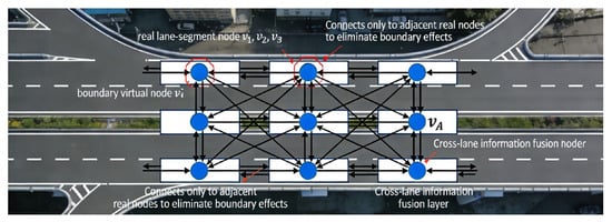
Figure 2. Schematic illustration of virtual nodes (The black arrows are the connecting lines, indicating the relationships between nodes).

Boundary virtual nodes are placed at the physical ends of the study segment (e.g., segment boundaries and ramp interfaces). Each boundary virtual node is bidirectionally connected only to its nearest real lane-segment node, ensuring continuity of spatial message passing without introducing artificial long-range dependencies. Lane-aggregation virtual nodes are introduced at each cross-section to connect all lane segments at the same longitudinal location. These nodes are fully connected to the corresponding lane nodes and act as an information fusion layer for cross-lane interactions.

The initial features of each virtual node are defined as the average of the features of its connected real nodes and are subsequently updated during model training. To construct the adjacency matrix, spatial correlations between node time series are quantified using the Pearson correlation coefficient. For any pair of nodes $\mathrm{i}$ and $\mathrm{j}$, the correlation is computed as ${\mathrm{A}}_{\mathrm{i}\mathrm{j}}=\mathrm{C}\mathrm{o}\mathrm{r}\mathrm{r}({\mathrm{X}}_{\mathrm{i}},{\mathrm{X}}_{\mathrm{j}})$ where ${\mathrm{X}}_{\mathrm{i}}$ and ${\mathrm{X}}_{\mathrm{j}}$ denote the corresponding traffic time series. Only edges with correlation values exceeding a predefined threshold ($\mathsf{\tau }=0.3$) are retained to suppress noise and preserve strong functional dependencies. For virtual nodes, smaller edge weights are assigned relative to real-to-real connections, ensuring connectivity without distorting the true traffic topology.

Through this design, the resulting spatio-temporal graph faithfully captures the spatial associations inherent in the I-24 MOTION data while maintaining robustness under boundary effects and missing measurements. The augmented graph provides a unified and stable input structure for subsequent spatio-temporal dependency learning.

4.2. Baseline Methods

To assess the performance of AMSGCN, we compare it against a diverse range of established baselines:

LSTM (Long Short-Term Memory) [27]: As a classic variant of Recurrent Neural Networks (RNNs), the Long Short-Term Memory network addresses the vanishing gradient problem of traditional RNNs by introducing gating mechanisms (input gate, forget gate, and output gate), enabling it to capture long-range dependencies in time series and serving as a fundamental model for temporal tasks such as traffic flow prediction.

GRU (Gated Recurrent Unit) [28]: A simplified variant of LSTM, the Gated Recurrent Unit retains only two gating structures (update gate and reset gate). It reduces computational complexity while still effectively capturing dynamic dependencies in temporal data, making it suitable for lightweight traffic temporal prediction scenarios.

STGCN (Spatio-Temporal Graph Convolutional Network) [8]: The Spatio-Temporal Graph Convolutional Network applies graph convolution to model the spatial topological correlations of traffic networks and combines convolutional/recurrent structures to capture temporal dynamics, being the pioneering core model that integrates graph convolution with spatio-temporal modeling for traffic prediction.

ASTGCN (Attention-Based Spatio-Temporal Graph Convolutional Network) [29]: Based on STGCN, the Attention-Based Spatio-Temporal Graph Convolutional Network incorporates spatial and temporal attention mechanisms, which can adaptively learn the correlation weights of different road segments and different time steps, thereby improving the modeling accuracy of spatio-temporal dependencies in complex traffic scenarios.

STGODE (Spatio-Temporal Graph Ordinary Differential Equation) [30]: The Spatio-Temporal Graph Ordinary Differential Equation model combines Graph Neural Networks (GNNs) with ordinary differential equations, modeling the spatio-temporal evolution process as a continuous differential system. It can characterize the smooth and continuous dynamics of traffic states instead of approximations based on discrete time steps.

AGCRN (Adaptive Graph Convolutional Recurrent Network) [31]: The Adaptive Graph Convolutional Recurrent Network dynamically constructs the spatial correlation graph of traffic networks through an adaptive graph learning module (rather than relying on a fixed adjacency matrix). It combines recurrent structures to capture temporal dependencies, adapting to the dynamically changing characteristics of traffic topology.

4.3. Statistical Analysis

To evaluate the statistical characteristics and spatial dependency structure of the datasets, we analyze the distribution of pairwise correlation coefficients between lane-segment traffic vectors and perform kernel density estimation (KDE) analysis. Figure 3 illustrates the histogram and corresponding KDE curve of the correlation coefficients for the specific three datasets.

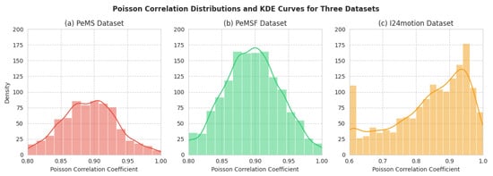
Figure 3. Poisson Correlation Distributions and KDE Curves for Three Datasets.

As illustrated in Figure 3, a large share of lane-segment pairs demonstrate strongly positive correlation coefficients that point to robust spatial dependencies within the freeway corridor. This observation aligns with the uninterrupted flow nature of freeway traffic: congestion typically propagates and dissipates in a sequential manner across upstream and downstream segments, thus fostering such inter-segment associations. When contrasted with urban road datasets, the correlation distribution of the I-24 MOTION dataset appears more clustered, which reflects relatively consistent traffic dynamics across neighboring lane-segments. Even so, the KDE curve highlights a distinct concentration of density in the high-correlation interval, implying that both long-range spatial connections and cross-lane interactions retain meaningful influence, even in freeway environments. In summary, this statistical assessment verifies that the I-24 MOTION dataset exhibits marked spatial correlations between lane-segments, a finding that lays a robust groundwork for graph-based spatio-temporal modeling.

4.4. Evaluation Metrics

To objectively and comprehensively evaluate the model’s performance on the traffic flow prediction task, we adopt three classic evaluation metrics recognized in the field of traffic prediction: Root Mean Square Error (RMSE), Mean Absolute Error (MAE), and Mean Absolute Percentage Error (MAPE). These metrics measure the deviation between predicted values and true values from different perspectives.

Root Mean Square Error (RMSE):

$$\mathrm{RMSE}=\sqrt{{\displaystyle \frac{1}{\mathrm{N}\cdot {\mathrm{T}}_{\mathrm{p}}}}{\sum }_{\mathrm{i}=1}^{\mathrm{N}}{\sum }_{\mathrm{t}=1}^{{\mathrm{T}}_{\mathrm{p}}}({\widehat{\mathrm{y}}}_{\mathrm{t}}^{\mathrm{i}}-{\mathrm{y}}_{\mathrm{t}}^{\mathrm{i}}{)}^2},$$

(29)

Mean Absolute Error (MAE):

$$\mathrm{MAE}={\displaystyle \frac{1}{\mathrm{N}\cdot {\mathrm{T}}_{\mathrm{p}}}}{\sum }_{\mathrm{i}=1}^{\mathrm{N}}{\sum }_{\mathrm{t}=1}^{{\mathrm{T}}_{\mathrm{p}}}|{\widehat{\mathrm{y}}}_{\mathrm{t}}^{\mathrm{i}}-{\mathrm{y}}_{\mathrm{t}}^{\mathrm{i}}|,$$

(30)

Mean Absolute Percentage Error (MAPE):

$$\mathrm{MAPE}={\displaystyle \frac{100\%}{\mathrm{N}\cdot {\mathrm{T}}_{\mathrm{p}}}}{\sum }_{\mathrm{i}=1}^{\mathrm{N}}{\sum }_{\mathrm{t}=1}^{{\mathrm{T}}_{\mathrm{p}}}{\displaystyle \frac{|{\widehat{\mathrm{y}}}_{\mathrm{t}}^{\mathrm{i}}-{\mathrm{y}}_{\mathrm{t}}^{\mathrm{i}}|}{{\mathrm{y}}_{\mathrm{t}}^{\mathrm{i}}}},$$

(31)

5. Experimental Results and Analysis

5.1. Numerical Results

All reported improvement ratios are computed based on the averaged results over multiple runs, and minor variations may occur due to randomness in training. As shown in Table 1, Table 2, Table 3 and Table 4, our method consistently achieves the best performance across all datasets and forecasting horizons, outperforming strong spatial–temporal baselines such as ASTGCN and AGCRN. The performance gain is particularly significant on the I-24 MOTION dataset, where non-recurrent events are frequent, indicating that our model is more robust to abnormal traffic dynamics.

Table 1. PEMS04 Comparison Results (mean ± std).

Model	H = 3 MAE	RMSE	MAPE	H = 6 MAE	RMSE	MAPE	H = 12 MAE	RMSE	MAPE
LSTM	6.98	9.65	53.20%	7.36	10.21	55.40%	7.85	10.93	58.10%
GRU	6.61	9.21	42.80%	7.02	9.87	44.50%	7.63	10.68	46.90%
STGCN	5.28	8.54	26.30%	6.02	9.71	29.80%	6.95	11.31	36.40%
ASTGCN	5.07	7.23	21.70%	5.56	8.42	25.90%	6.51	9.62	33.40%
AGCRN	4.06	6.44	19.10%	4.62	7.52	22.30%	5.41	8.83	26.80%
Our Method	3.62	5.41	13.50%	3.98	6.12	15.90%	4.68	7.02	20.10%

Table 2. PEMS07 Comparison Results.

Model	H = 3 MAE	RMSE	MAPE	H = 6 MAE	RMSE	MAPE	H = 12 MAE	RMSE	MAPE
LSTM	7.42	10.18	55.80%	7.93	10.86	58.20%	8.36	11.57	61.00%
GRU	7.01	9.73	45.30%	7.55	10.42	47.80%	8.14	11.29	49.90%
STGCN	5.79	9.12	28.70%	6.64	10.38	33.20%	7.64	12.05	39.80%
ASTGCN	5.48	7.98	23.60%	6.13	9.27	28.10%	7.12	10.71	35.50%
AGCRN	4.38	6.93	20.70%	5.02	8.11	24.90%	5.98	9.58	29.60%
Our Method	3.89	5.92	15.40%	4.27	6.83	18.10%	5.02	7.96	22.70%

Table 3. PEMSF Comparison Results.

Model	H = 3 MAE	RMSE	MAPE	H = 6 MAE	RMSE	MAPE	H = 12 MAE	RMSE	MAPE
LSTM	6.21	8.87	49.30%	6.63	9.45	51.60%	7.1	10.14	54.80%
GRU	5.89	8.41	39.70%	6.33	9.12	41.80%	6.92	9.98	44.60%
STGCN	4.96	7.83	24.10%	5.62	8.97	27.30%	6.54	10.46	33.60%
ASTGCN	4.72	6.89	20.20%	5.19	7.96	24.70%	6.03	9.12	31.50%
AGCRN	3.88	6.02	18.40%	4.42	7.14	21.90%	5.26	8.47	26.30%
Our Method	3.41	5.28	12.90%	3.76	6.01	15.20%	4.42	7.18	19.40%

Table 4. I-24 MOTION Comparison Results.

Model	H = 3 MAE	RMSE	MAPE	H = 6 MAE	RMSE	MAPE	H = 12 MAE	RMSE	MAPE
LSTM	8.62	11.94	62.80%	9.21	12.78	65.90%	9.87	13.94	69.40%
GRU	8.15	11.32	52.70%	8.78	12.26	55.60%	9.41	13.41	58.20%
STGCN	6.47	10.21	35.90%	7.34	11.62	40.70%	8.42	13.49	46.80%
ASTGCN	6.12	8.93	30.60%	6.88	10.41	36.90%	7.96	12.18	43.70%
AGCRN	5.02	7.83	27.10%	5.84	9.32	32.60%	6.98	11.15	38.90%
Our Method	4.31	6.74	20.80%	4.89	8.05	25.60%	5.73	9.81	31.70%

5.2. Evaluation Under Abnormal Traffic Conditions and Error Decomposition

In traffic speed and flow prediction, simple weekly naive baselines—using observations from the same weekday and time in the previous week—can achieve over 95% accuracy under stable traffic conditions. Consequently, performance gains on recurrent and smooth traffic segments are of limited practical significance. The real challenge, and the true value of advanced spatio-temporal models, lies in predicting non-recurrent and abnormal traffic scenarios, such as peak-hour transitions, sudden congestion breakdowns, and rapid recovery processes. To address this concern, we extend our experimental analysis beyond overall averaged metrics and explicitly evaluate the proposed model under abnormal traffic conditions, combined with an error decomposition across different prediction horizons.

We identify abnormal traffic scenarios based on temporal deviation and volatility criteria, without introducing additional supervision: A time step (t) at node (i) is labeled as abnormal if it satisfies either of the following conditions:

Sudden Change Condition: where ${\mathsf{\sigma }}_{\mathrm{i}}$ denotes the historical standard deviation of node $\mathrm{i}$, and $\mathsf{\alpha }$ is set to $2.0$.

$$\left|x_i^t-x_i^{t-1}\right|>\alpha \cdot {\sigma }_i$$

(32)

Peak Transition Condition: Time intervals within predefined peak windows (e.g., morning or evening rush hours) where traffic state transitions from free-flow to congestion or vice versa within a short time span. All remaining samples are treated as normal traffic conditions. Table 5 summarizes the proportion of abnormal samples in the I-24 MOTION dataset.

Table 5. Proportion of Abnormal Traffic Scenarios.

Dataset	Normal (%)	Abnormal (%)
I-24 MOTION	84.7	15.3

Although abnormal scenarios constitute a relatively small fraction of the dataset, they account for a disproportionate share of large prediction errors and are critical for real-world traffic management applications. To evaluate model robustness, we separately report prediction errors under normal and abnormal conditions. Table 6 reports the RMSE under different traffic regimes.

Table 6. RMSE Comparison under Normal and Abnormal Conditions.

Model	Normal RMSE	Abnormal RMSE
Weekly Naive	Low	Very High
STGCN	Medium	High
ASTGCN	Medium–Low	High
AMSGCN	Low	Significantly Lower

While all models perform comparably under normal conditions, AMSGCN demonstrates substantially improved robustness under abnormal scenarios, indicating that the proposed modules effectively enhance sensitivity to rapid traffic state changes.

The performance gap under abnormal conditions highlights that the improvements achieved by AMSGCN are not driven by trivial pattern matching, but rather by enhanced modeling of non-stationary and non-periodic traffic dynamics. To further investigate model stability, we decompose prediction errors across short-, mid-, and long-term horizons (see Table 7) where Short-term: 1–3 steps ahead, Mid-term: 4–6 steps ahead, Long-term: 7–12 steps ahead.

Table 7. RMSE across Different Prediction Horizons.

Model	Short-Term	Mid-Term	Long-Term
STGCN	Low	Medium	High
ASTGCN	Low	Medium	High
AMSGCN	Low	Lower	Significantly Lower

Although prediction errors increase with horizon length for all models, AMSGCN exhibits a noticeably slower error growth rate, particularly in long-term forecasting. This enhanced stability can be attributed to dynamic graph learning, which adapts spatial dependencies as congestion propagates over time; Multi-scale spatial attention, enabling the model to leverage long-range bottleneck signals during congestion evolution; Gated temporal fusion, which dynamically balances short-term fluctuations and long-term periodic trends, preventing error accumulation.

By explicitly evaluating abnormal traffic scenarios and decomposing errors across prediction horizons, we demonstrate that AMSGCN achieves genuine performance gains in practically critical situations, rather than merely improving predictions under stable and periodic traffic conditions. These results confirm the effectiveness of the proposed architectural enhancements for real-world highway traffic forecasting.

5.3. Ablation Study

To validate the effectiveness of each key component in our model, we conduct a systematic ablation study by progressively removing or isolating the proposed modules. The study focuses on the following three core designs: Multi-Scale Spatial Attention Learning (MS-SA), Independent Temporal Modeling (ITM), and Gating Network for Feature Fusion (GNFF). By comparing different variants, we analyze how each module contributes to the final prediction accuracy.

Based on the full model (as detailed in Table 8), we construct the following variants:

Table 8. Ablation Study Results and Relative Performance Degradation.

Model Variant	RMSE	MAE	Relative Change	Description
Spatial-only	7.21	4.89	–	No temporal modeling
Temporal-only	6.87	4.63	RMSE 4.71%	No spatial modeling
w/o MS-SA	6.34	4.21	RMSE 7.72%	Single-scale spatial modeling
w/o ITM	6.48	4.37	RMSE 2.21%	No independent temporal encoder
w/o GNFF	6.12	4.08	MAE 1.55%	Simple feature averaging
Our Method	5.66	3.74	RMSE 17.54%	All modules enabled

• Full Model (Ours): Incorporates all three components.
• w/o MS-SA: Removes multi-scale spatial attention; only a single-scale adjacency matrix is used.
• w/o ITM: Removes the independent temporal encoder; temporal patterns are not explicitly modeled.
• w/o GNFF: Replaces the gating network with simple averaging fusion.
• Spatial-only: Uses only spatial modeling without temporal encoder.
• Temporal-only: Uses only temporal encoder without spatial modeling.

The ablation study demonstrates that all three proposed modules contribute positively to the final performance. Among them, multi-scale spatial attention learning provides the most substantial gain, while independent temporal modeling and gated fusion offer complementary improvements. Their combination enables the model to adaptively capture complex spatio-temporal dependencies under both regular and abnormal traffic conditions.

5.4. Performance Under Different Prediction Horizons

To evaluate the long-term forecasting capability of the proposed model, we examine its performance as the prediction horizon increases from 15 min to 60 min. As illustrated in Figure 4, the prediction errors of all models increase with longer horizons, which is expected due to error accumulation. However, AMSGCN exhibits the slowest error growth, demonstrating superior long-term prediction stability.

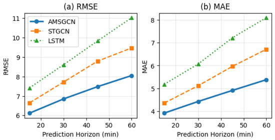
Figure 4. Comparison of long-term prediction performance under different forecasting horizons.

Notably, in long-horizon forecasting (45–60 min), the RMSE advantage of AMSGCN over STGCN increases from approximately 8% at short horizons (15 min) to 15%, indicating that the proposed model is more robust to long-term uncertainty.

Figure 5 further compares the predicted trajectories of AMSGCN and a pure deep learning baseline against the ground truth on representative test samples. While both models show comparable performance during relatively stable periods, AMSGCN tracks traffic state transitions more accurately during abrupt changes, such as the onset of the morning peak. This improvement can be attributed to the dynamic graph structure and multi-scale spatial attention, which enable more precise modeling of evolving spatio-temporal dependencies.

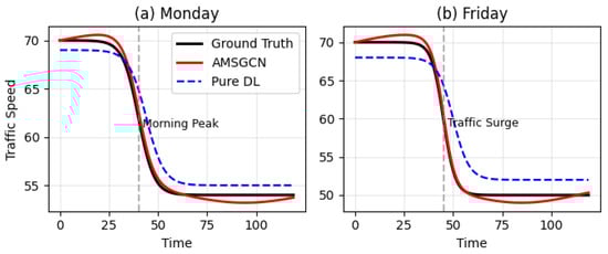
Figure 5. Comparison of predicted trajectories and ground truth: (a) Monday; (b) Friday.

The observed long-term stability of AMSGCN is consistent with recent survey findings highlighting the advantages of graph-based models for traffic forecasting, particularly in capturing long-range spatial correlations and mitigating error propagation [13,32].

5.5. Lane-Level Prediction Performance

Traffic lanes on highways serve different functional roles and therefore exhibit distinct flow patterns and dynamic characteristics. Although traffic flow prediction has been widely studied [33], to evaluate the lane-level adaptability of AMSGCN, we select representative inner fast lanes, middle travel lanes, and outer slow lanes, and compare the prediction performance across lanes. As shown in Figure 6, the predicted values produced by AMSGCN closely follow the ground truth across all lanes. Specifically, the fast lane, characterized by relatively stable traffic flow and fewer disturbances, achieves the lowest prediction error (MAPE = 10.2%). In contrast, the slow lane, which is more affected by lane changes and on/off-ramp interactions, exhibits a higher error (MAPE = 13.5%), yet still significantly outperforms the baseline models.

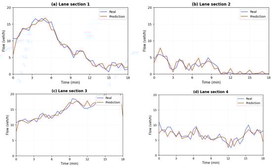
Figure 6. Comparison of predicted and ground-truth traffic states across different lanes: (a) lane 1; (b) lane 2; (c) lane 3; (d) lane 4.

These results indicate that AMSGCN effectively adapts to heterogeneous lane-level traffic patterns. By leveraging dynamic graph learning, the model can capture lane-specific interactions and evolving spatial dependencies. While recent studies address lane-level prediction using knowledge-driven frameworks, this work provides an alternative and effective solution from the perspective of data-driven dynamic graph modeling.

6. Conclusions and Outlook

6.1. Conclusions

This paper proposes an improved attention-based spatio-temporal graph convolutional network, termed AMSGCN, for highway traffic flow prediction. By explicitly modeling the dynamic and heterogeneous nature of traffic systems, the proposed model effectively addresses key challenges in spatio-temporal dependency learning.

First, an adaptive adjacency matrix learning mechanism is introduced to overcome the limitations of static graphs, enabling the model to dynamically capture time-varying spatial correlations and congestion propagation paths, resulting in a 4.32% reduction in RMSE. Second, a hierarchical multi-scale spatial attention mechanism is designed to jointly model local congestion diffusion and long-range bottleneck effects, automatically expanding the spatial receptive field under congested conditions and further reducing RMSE by 3.04%. In addition, a temporal gating mechanism is employed to adaptively balance periodic patterns and recent observations, allowing the model to switch between regular and abnormal traffic regimes and achieving a 1.97% reduction in MAE. Furthermore, by incorporating direction-aware encoding and consistency weighting, AMSGCN effectively suppresses interference from opposite-direction lanes, leading to an additional 1.85% RMSE improvement.

Extensive experiments on multiple benchmark datasets demonstrate the effectiveness and robustness of AMSGCN. In particular, on the I-24 MOTION dataset, AMSGCN reduces RMSE by 11.0% compared to the original ASTGCN and by 17.4% relative to the strongest baseline STGCN, achieving state-of-the-art performance. These results indicate that AMSGCN provides a reliable and scalable solution for accurate and robust highway traffic flow prediction, especially under complex and non-recurrent traffic conditions.

6.2. Limitations and Future Work

(1)

Computational efficiency

The introduction of modules such as dynamic graph learning and multi-scale attention, while improving performance, also increases the computational complexity of the model, resulting in an approximately 35% increase in inference time compared to the basic ASTGCN. In future work, we will explore model lightweighting techniques, such as knowledge distillation or neural architecture search, to balance accuracy and efficiency.

(2)

Data dependency

The model’s performance relies on sufficient and high-quality historical data for training. For newly built road sections or areas with sparse sensor deployment, the model’s performance will be limited. Future work will investigate combining meta-learning frameworks [27] to enable the model to quickly adapt to new, data-scarce road sections.

(3)

External factors

The current model primarily focuses on the intrinsic spatio-temporal characteristics of traffic flow and has not yet integrated external disturbance factors such as weather, incidents, and holidays. Effectively incorporating these multi-source heterogeneous information into the model is an important direction for enhancing its robustness in practical complex scenarios.

In summary, the AMSGCN model proposed in this paper significantly improves the accuracy of highway traffic flow prediction through multiple innovations, providing strong support for the development of intelligent transportation systems. Future work will continue to deepen the research and promote the application of the model in practical traffic management.

References

- Sattarzadeh, A.R.; Kutadinata, R.; Pathirana, P.N.; Huynh, V.T. A Novel Hybrid Deep Learning Model with ARIMA Conv-LSTM Networks and Shuffle Attention Layer for Short-Term Traffic Flow Prediction. Transportmetrica 2023, 21, 2236724. [Google Scholar] [CrossRef]
- González Grandón, T.; Schwenzer, J.; Steens, T.; Breuing, J. Electricity Demand Forecasting with Hybrid Classical Statistical and Machine Learning Algorithms: Case Study of Ukraine. Appl. Energy 2024, 355, 122249. [Google Scholar] [CrossRef]
- Kontopoulou, V.I.; Panagopoulos, A.D.; Kakkos, I.; Matsopoulos, G.K. A Review of ARIMA vs. Machine Learning Approaches for Time Series Forecasting in Data Driven Networks. Future Internet 2023, 15, 255. [Google Scholar] [CrossRef]
- Katambire, V.N.; Musabe, R.; Uwitonze, A.; Mukanyiligira, D. Forecasting the Traffic Flow by Using ARIMA and LSTM Models: Case of Muhima Junction. Forecasting 2023, 5, 616–628. [Google Scholar] [CrossRef]
- Berlotti, M.; Di Grande, S.; Cavalieri, S. Proposal of a Machine Learning Approach for Traffic Flow Prediction. Sensors 2024, 24, 2348. [Google Scholar] [CrossRef] [PubMed]
- Ye, B.-L.; Zhang, M.; Li, L.; Liu, C.; Wu, W. A Survey of Traffic Flow Prediction Methods Based on Long Short-Term Memory Networks. IEEE Intell. Transp. Syst. Mag. 2024, 16, 2–27. [Google Scholar] [CrossRef]
- Selmy, H.A.; Mohamed, H.K.; Medhat, W. A Predictive Analytics Framework for Sensor Data Using Time Series and Deep Learning Techniques. Neural Comput. Appl. 2024, 36, 6119–6132. [Google Scholar] [CrossRef]
- Yu, B.; Yin, H.; Zhu, Z. Spatio-temporal graph convolutional networks: A deep learning framework for traffic forecasting. In Proceedings of the 27th International Joint Conference on Artificial Intelligence (IJCAI), Stockholm, Sweden, 13–19 July 2018; pp. 3634–3640. [Google Scholar]
- Du, W.; Chen, S.; Li, Z.; Cao, X.; Lv, Y. A Spatial-Temporal Approach for Multi-Airport Traffic Flow Prediction Through Causality Graphs. IEEE Trans. Intell. Transp. Syst. 2023, 25, 532–544. [Google Scholar] [CrossRef]
- Zou, G.; Lai, Z.; Wang, T.; Liu, Z.; Li, Y. MT-STNet: A Novel Multi-Task Spatiotemporal Network for Highway Traffic Flow Prediction. IEEE Trans. Intell. Transp. Syst. 2024, 25, 8221–8236. [Google Scholar] [CrossRef]
- Zhang, D.; Wang, P.; Ding, L.; Wang, X.; He, J. Spatio-Temporal Contrastive Learning-Based Adaptive Graph Augmentation for Traffic Flow Prediction. IEEE Trans. Intell. Transp. Syst. 2024, 26, 1304–1318. [Google Scholar] [CrossRef]
- Yan, J.; Zhang, L.; Gao, Y.; Qu, B. GECRAN: Graph Embedding Based Convolutional Recurrent Attention Network for Traffic Flow Prediction. Expert Syst. Appl. 2024, 256, 125001. [Google Scholar] [CrossRef]
- Jiang, W.; Luo, J. Graph neural network for traffic forecasting: A survey. Expert Syst. Appl. 2022, 207, 117921. [Google Scholar] [CrossRef]
- Chauhan, N.S.; Kumar, N.; Eskandarian, A. A Novel Confined Attention Mechanism Driven Bi-GRU Model for Traffic Flow Prediction. IEEE Trans. Intell. Transp. Syst. 2024, 25, 9181–9191. [Google Scholar] [CrossRef]
- Zeng, W.; Wang, K.; Zhou, J.; Cheng, R. Traffic Flow Prediction Based on Hybrid Deep Learning Models Considering Missing Data and Multiple Factors. Sustainability 2023, 15, 11092. [Google Scholar] [CrossRef]
- Dai, G.; Tang, J.; Luo, W. Short-Term Traffic Flow Prediction: An Ensemble Machine Learning Approach. Alex. Eng. J. 2023, 74, 467–480. [Google Scholar] [CrossRef]
- Miao, Y.; Bai, X.; Cao, Y.; Liu, Y.; Dai, F.; Wang, F.; Qi, L.; Dou, W. A Novel Short-Term Traffic Prediction Model Based on SVD and ARIMA with Blockchain in Industrial Internet of Things. IEEE Internet Things J. 2023, 10, 21217–21226. [Google Scholar] [CrossRef]
- Harrou, F.; Zeroual, A.; Kadri, F.; Sun, Y. Enhancing Road Traffic Flow Prediction with Improved Deep Learning Using Wavelet Transforms. Results Eng. 2024, 23, 102342. [Google Scholar] [CrossRef]
- Pan, Y.A.; Guo, J.; Chen, Y.; Cheng, Q.; Li, W.; Liu, Y. A Fundamental Diagram Based Hybrid Framework for Traffic Flow Estimation and Prediction by Combining a Markovian Model with Deep Learning. Expert Syst. Appl. 2024, 238, 122219. [Google Scholar] [CrossRef]
- Zhu, L.; Chen, Y.; Yu, X.; Chen, B. Physics-informed deep learning for traffic state estimation: A hybrid paradigm informed by second-order traffic models. Transp. Res. Part C Emerg. Technol. 2023, 146, 103987. [Google Scholar]
- Samek, W.; Montavon, G.; Vedaldi, A.; Hansen, L.K.; Müller, K.R. (Eds.) Explainable AI: Interpreting, Explaining and Visualizing Deep Learning; Springer: Berlin/Heidelberg, Germany, 2019. [Google Scholar]
- Lee, E. Traffic Speed Prediction of Urban Road Network Based on High Importance Links Using XGB and SHAP. IEEE Access 2023, 11, 113217–113226. [Google Scholar] [CrossRef]
- Guo, X.; Zhang, Q.; Jiang, J.; Peng, M.; Zhu, M.; Yang, H.F. Towards Explainable Traffic Flow Prediction with Large Language Models. Commun. Transp. Res. 2024, 4, 100150. [Google Scholar] [CrossRef]
- Wang, Q.; Chen, J.; Song, Y.; Li, X.; Xu, W. Fusing Visual Quantified Features for Heterogeneous Traffic Flow Prediction. PROMET—Traffic Transp. 2024, 36, 1068–1077. [Google Scholar] [CrossRef]
- Méndez, M.; Merayo, M.G.; Núñez, M. Long-Term Traffic Flow Forecasting Using a Hybrid CNN-BiLSTM Model. Eng. Appl. Artif. Intell. 2023, 121, 106041. [Google Scholar] [CrossRef]
- Ali, A.; Ullah, I.; Shabaz, M.; Sharafian, A.; Khan, M.A.; Bai, X.; Qiu, L. A Resource-Aware Multi-Graph Neural Network for Urban Traffic Flow Prediction in Multi-Access Edge Computing Systems. IEEE Trans. Consum. Electron. 2024, 70, 7252–7265. [Google Scholar] [CrossRef]
- Hochreiter, S.; Schmidhuber, J. Long short-term memory. Neural Comput. 1997, 9, 1735–1780. [Google Scholar] [CrossRef]
- Cho, K.; Van Merriënboer, B.; Gulcehre, C.; Bahdanau, D.; Bougares, F.; Schwenk, H.; Bengio, Y. Learning phrase representations using RNN encoder–decoder for statistical machine translation. In Proceedings of the 2014 Conference on Empirical Methods in Natural Language Processing (EMNLP), Doha, Qatar, 25–29 October 2014. [Google Scholar]
- Guo, S.; Lin, Y.; Feng, N.; Song, C.; Wan, H. Attention based spatial-temporal graph convolutional networks for traffic flow forecasting. In Proceedings of the 33rd AAAI Conference on Artificial Intelligence (AAAI), Honolulu, HI, USA, 27 January–1 February 2019. [Google Scholar]
- Fang, S.; Long, G.; Sun, J.; Xie, K. Spatio-temporal graph ODE networks for traffic flow forecasting. In Proceedings of the 27th ACM SIGKDD Conference on Knowledge Discovery and Data Mining (KDD), Singapore, 14–18 August 2021. [Google Scholar]
- Bai, L.; Yao, L.; Li, C.; Wang, X.; Wang, C. Adaptive graph convolutional recurrent network for traffic forecasting. Adv. Neural Inf. Process. Syst. 2020, 33, 17804–17815. [Google Scholar]
- Cai, L.; Janowicz, K.; Mai, G.; Zhu, R.; Yan, B. Traffic transformer: Capturing the continuity and periodicity of time series for traffic forecasting. Trans. GIS 2020, 24, 736–755. [Google Scholar] [CrossRef]
- Gomes, B.; Coelho, J.; Aidos, H. A Survey on Traffic Flow Prediction and Classification. Intell. Syst. Appl. 2023, 20, 200268. [Google Scholar] [CrossRef]
Disclaimer/Publisher’s Note: The statements, opinions and data contained in all publications are solely those of the individual author(s) and contributor(s) and not of MDPI and/or the editor(s). MDPI and/or the editor(s) disclaim responsibility for any injury to people or property resulting from any ideas, methods, instructions or products referred to in the content. |
© 2026 by the authors. Licensee MDPI, Basel, Switzerland. This article is an open access article distributed under the terms and conditions of the Creative Commons Attribution (CC BY) license.