Linear-Region-Based Contour Tracking for Edge Images

Abstract

This work presents the Linear-Region-Based Contour Tracking (LRCT) method for extracting external contours in images, designed to achieve an accurate and efficient description of shapes, particularly useful for archaeological materials with irregular geometries. The approach treats the contour as a discrete signal and analyzes image regions containing edge segments. From these regions, a local linear model is estimated to guide the selection and chaining of representative pixels, yielding a continuous perimeter trajectory. This strategy reduces the amount of data required to describe the contour without compromising shape fidelity. As a case study, the method was applied to images of replicas of archaeological materials exhibiting substantial variations in color and morphology. The results show that the obtained trajectories are comparable in quality to those obtained using classical pipelines based on Canny edge detection followed by Moore tracing, while providing more compact representations well suited for subsequent analyses. Consequently, the method offers an efficient and reproducible alternative for documentation, recording, and morphological comparison, strengthening data-driven approaches in archaeological research.

1. Introduction

Contour characterization is a fundamental technique in classical computer vision, as it enables the generation of structured information about the entities present in a visual scene. The numerical description of a contour can be approached from multiple criteria, with applications ranging from shape comparison and similarity assessment to industrial quality control. Although numerous methods for edge detection have been developed—such as first-derivative operators [1]—the geometric and mathematical properties associated with contours are sufficiently broad and complex to justify continued research from complementary methodological perspectives.

A contour is an abstract feature that emerges when a three-dimensional scene from the real world is projected onto a two-dimensional image, manifesting as a boundary that delimits differences in visual properties such as color, texture, or intensity. In this context, it is important to distinguish between an edge and a contour, two terms that should not be treated as synonymous. Edges correspond to points where a significant change in these properties occurs, even within the surface of a single object. Contours, by contrast, describe the complete periphery of an entity and define its overall shape. Their analysis typically involves two consecutive procedures: edge detection and contour parameterization.

Classical detection methods are grounded in the idea that change is the essential characteristic to identify a boundary in an image. Consequently, they rely on the discrete differentiation of visual content, implicit in gradient computation, and implemented through operators such as Sobel and Prewitt, the Laplacian operator, or frequency-domain filtering via the Discrete Fourier Transform. The result of these operations is an image in which pixels without significant variation are suppressed, while those exhibiting abrupt changes are highlighted. However, this process is sensitive to noise, which can produce disconnected or inconsistent edges. As a result, further refinement is required to remove false positives and retain only the edges relevant for contour reconstruction. Once an edge image is obtained, chaining methods reconstruct the perimeter by performing a unidirectional search along the trajectory, listing the coordinates of the detected points to represent the shape of the object in a continuous and structured manner.

In this context, this article incorporates two stages within the classical contour-extraction workflow, focusing on contour tracking from an edge map obtained through a statistically motivated thresholding scheme under moderate noise conditions. This edge map serves as a robust input for the subsequent processing stage. In a second stage, a contour-following method based on the estimation of representative lines along the sequence of edge points is proposed, without requiring a precomputed thinned or explicitly connected contour representation. Each line acts as a local model and provides directional information that guides the prediction and adjustment of the next position along the perimeter, yielding a compact and representative contour description.

When applied to closed contours, and provided that a sufficient visual separation exists between edge and noise, the procedure reliably returns to the initial search point. The method exhibits particularly stable performance on contours without abrupt transitions, especially those with irregular geometries and smooth shape variations. To validate the approach, archaeological materials were selected in which the general shape of the objects was prioritized over minor edge details. As an example of application, the results are illustrated using both replicas of artifacts and materials commonly found in archaeological contexts.

Although this proposal is developed in a period in which deep learning (DL)-based methods dominate many computer vision applications, the present work focuses on a classical, model-based approach intended for scenarios where transparency, controllability of processing steps, and low computational requirements are essential. The method is not intended to replace contour-extraction frameworks based on convolutional neural networks (CNNs), but to operate in situations involving controlled acquisition conditions, limited or nonexistent training datasets, restrictions on computational resources such as the absence of graphics processing unit (GPU) acceleration, or cases in which direct intervention in the processing sequence is required to adjust parameters and optimize the outcome.

Within this context, the present work proposes LRCT, a modular method integrated into the classical computer vision processing pipeline, guided by mathematical principles for contour parameterization and with strong potential for applications in archaeological documentation and recording.

2. Related Work

Edge detection is a fundamental component of computer vision systems, with an importance comparable to color estimation and geometric characterization for the qualitative and quantitative description of a scene. Throughout the evolution of the field, numerous general-purpose methods have been developed, which, through specific adjustments, can be adapted to various types of images and acquisition conditions. These algorithms have established a solid methodological foundation that continues to be employed and expanded across multiple research directions.

This section introduces the classical principles associated with edge detection and contour tracing, as well as some of their most representative applications. It also provides a brief contextualization of the proposed method, highlighting its relationship to previous approaches and the needs that motivate its development.

2.1. Classical Algorithms and Foundational Principles

In traditional computer vision approaches, edge detection and contour characterization are typically formulated as a sequential process. In the first stage, significant intensity transitions are identified to generate a binary image; subsequently, these points are organized through a chaining procedure that reconstructs the path of the contour. This workflow has led to a variety of algorithms that differ in accuracy, robustness to noise, and computational efficiency.

The earliest methods—still widely used—were based on derivative operators applied to grayscale images, designed to respond to local intensity changes. Among the most representative are the first-order operators Sobel [2] and Prewitt [3], which approximate the gradient through simple convolution masks. Second-order operators, such as the Laplacian, have also been employed; these highlight abrupt changes in intensity curvature and facilitate the detection of pronounced transitions [4].

A decisive advancement is the Canny algorithm [5], widely recognized for its ability to generate continuous, thin, and stable edges even under moderate noise conditions. Its design integrates Gaussian filtering, precise gradient estimation, non-maximum suppression, and hysteresis thresholding. However, Canny only identifies the pixels belonging to the edge and therefore requires additional methods to trace and organize these points into coherent trajectories.

In this context, contour-tracing methods operate on a previously cleaned binary edge image, commonly produced by gradient-based detectors such as Canny. Their goal is to follow the perimeter, ensure the continuity of the trace, and estimate the local edge direction. Among the most representative algorithms are Moore–Neighbor Tracing and the chain-code boundary descriptor attributed to Fu et al., whose formulation is widely reported in classical computer vision textbooks, such as Pajares and De la Cruz [1]. The Moore algorithm explores the eight-neighbor region around each edge pixel, enabling the reconstruction of closed contours through an ordered and continuous chain. Its simplicity has contributed to its adoption in widely used tools, such as the bwboundaries function in MATLAB (MathWorks, Natick, MA, USA) [6]. In contrast, the method by Fu et al. introduces decision rules aimed at producing more compact contour representations, reducing the number of points without compromising geometric fidelity.

By contrast, region-based contour extraction methods operate on binary images obtained through object segmentation rather than edge detection. In this context, Suzuki and Abe [7] proposed contour extraction directly from segmented binary regions, exploiting the contrast between the object of interest and its surrounding background, which enables the use of global or adaptive thresholding. The contour is obtained through a systematic traversal of the region boundaries, employing algorithms such as Moore-neighbor tracing or region-based border-following techniques. Numerous modern implementations of contour tracing, including those available in OpenCV (OpenCV.org, Palo Alto, CA, USA) and MATLAB, efficiently incorporate this strategy. However, these approaches rely on accurate binary segmentation, which can be challenging in scenarios affected by illumination variations, reflections, or color changes.

There are also approaches that do not rely on an explicit chaining stage and instead directly fit geometric models to the detected edge points or parametrize the shape using the available samples. The Hough Transform [8] allows for the identification of simple geometric structures through a parameter space that accumulates evidence of dominant lines or curves. Although effective for regular shapes, it does not perform sequential contour tracing. To mitigate its high computational cost, Fernandes and Oliveira [9] developed a deterministic variant that groups collinear pixels and improves efficiency, while maintaining the focus on idealized geometric structures.

2.2. Recent Research and Current Developments

Although classical algorithms offer satisfactory results in controlled environments, their application in real-world scenarios often requires additional adaptations. Consequently, several studies have revisited and extended these methods to address specific needs across various domains.

Li et al. [10] propose the Contrast-Invariant Edge Detection (CIED) method for medical imaging, integrating Gaussian filtering, morphological operations, and fusion of the most significant bit planes (MSB). This approach increases robustness against contrast variations and promotes the extraction of continuous and structurally coherent edges.

In a direction related to the present work, Li et al. [11] introduce an adaptive segmentation scheme that divides the image into regions of interest based on local features—such as texture and contrast—to apply region-specific filters and dynamic thresholds. The method demonstrates robustness to lighting variations in images of mechanical components.

In the domain of aerial photography, Crommelinck et al. [12] evaluated different methods for cadastral boundary delineation and concluded that the well-established gPb–owt–ucm framework offers the highest geometric accuracy. Nevertheless, its considerable computational cost and the need for manual intervention limit its applicability in operational scenarios.

For compact contour tracing, Seo et al. [13] developed a method oriented toward resource-constrained devices. Their approach enables tracing and storing contours in a compact representation and recovering them with high accuracy even in regions of high curvature, although specific cases remain in which certain contours fail to be detected.

From a bio-inspired perspective, Sun et al. [14] introduced an approach based on superpixels to generate candidate contour segments, evaluated through a model that integrates low-level information with perceptual principles. This method achieves competitive results but exhibits limitations in some scenarios.

Bridging classical methods and modern deep-learning-based approaches, Freitas et al. [15] combine specialized convolutional models (RINDNet and SobelU-Net) with the classical “shortest path” algorithm, improving breast-edge detection in clinical images and enhancing generalization across heterogeneous datasets.

The proposed method, framed within classical computer vision, is inspired by the perceptual tracing of contours performed by a human observer. It is organized into two stages: manual image preparation and contour characterization. Unlike traditional approaches, it does not restrict itself to the immediate eight-pixel neighborhood but instead considers larger regions that preserve the global trend of the contour. In this way, individual pixels are replaced by a representative sampling that reduces computational load and facilitates its application in archaeological recording, producing a more compact mathematical representation that is comparable across pieces with similar morphologies.

3. Method

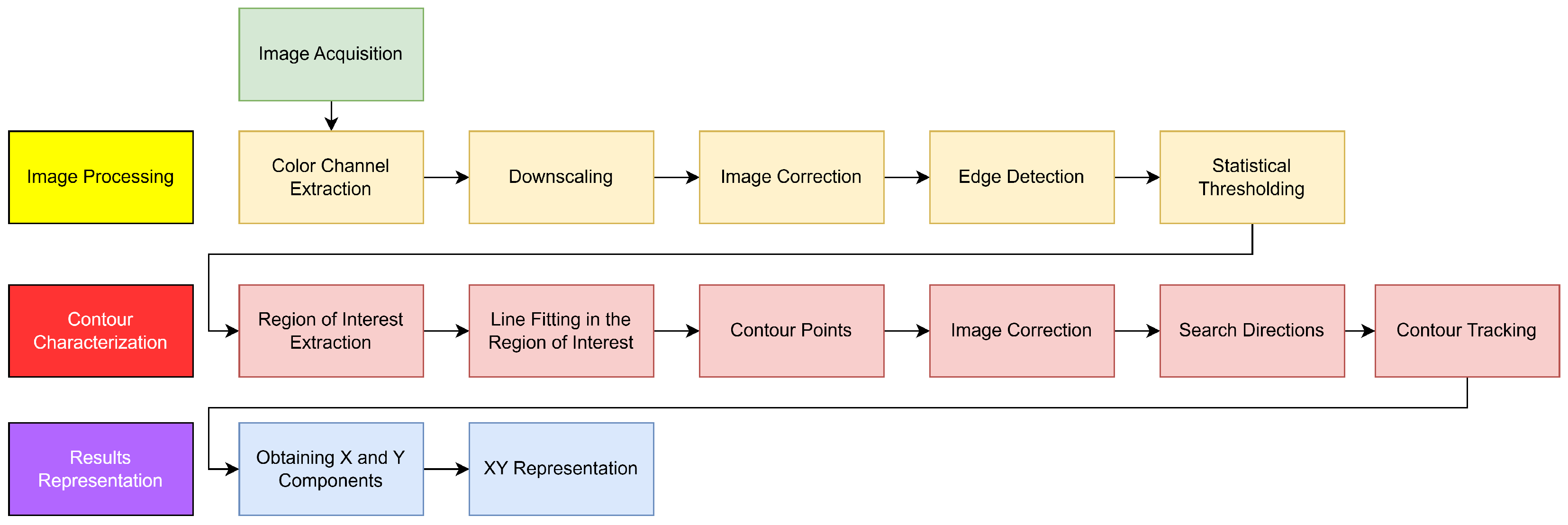
This section describes the procedure used to obtain the sequence of coordinate pairs $(x,y)$ representing the contour of an entity from a digital image. As illustrated in Figure 1, the method is organized into a pipeline composed of three main stages, each with adjustable parameters that allow adaptation to the characteristics of the scene and ensure result accuracy.

Figure 1. Stages of the proposed algorithm.

The first stage, referred to as Image Processing, encompasses the fundamental operations of the classical computer vision pipeline, aiming to enhance relevant features prior to contour parametrization. In the literature, this stage is commonly associated with Edge Detection due to its role in delineating regions of interest through filtering, contrast enhancement, and gradient analysis.

The second stage, Contour Characterization, converts the edge-derived information into a geometric representation by chaining points according to their spatial continuity and intensity consistency, ultimately generating a numerical description of the contour. This process follows the classical computer vision principle wherein the output transitions from an image to a mathematical interpretation.

Finally, the Result Presentation stage organizes and displays the generated geometric characterization, providing parameters ready for subsequent analysis or integration into specific applications. This stage facilitates data interpretation and enables comparison or evaluation.

3.1. Image Processing

Image processing constitutes a fundamental stage of the pipeline, as it establishes the conditions required for proper edge detection and contour characterization. The following section describes the applied operations and their common variants, which can be adapted based on the desired level of precision and available computational resources. In general, this stage aims to reduce data volume, increase object-background contrast, and facilitate edge identification.

3.1.1. Image Acquisition

Prior to capture, environmental conditions should be controlled using stable lighting, high-contrast backgrounds, and appropriate camera settings, including capture distance and possible optical filters (Wibowo et al. [16]). The initial image, represented by the function $f_0$ in Equation (1), assigns each coordinate $(x,y)$ the intensity of its three color components.

$$f_0:{\mathbb{Z}}^2\to {\{0,1,\dots ,255\}}^3$$

(1)

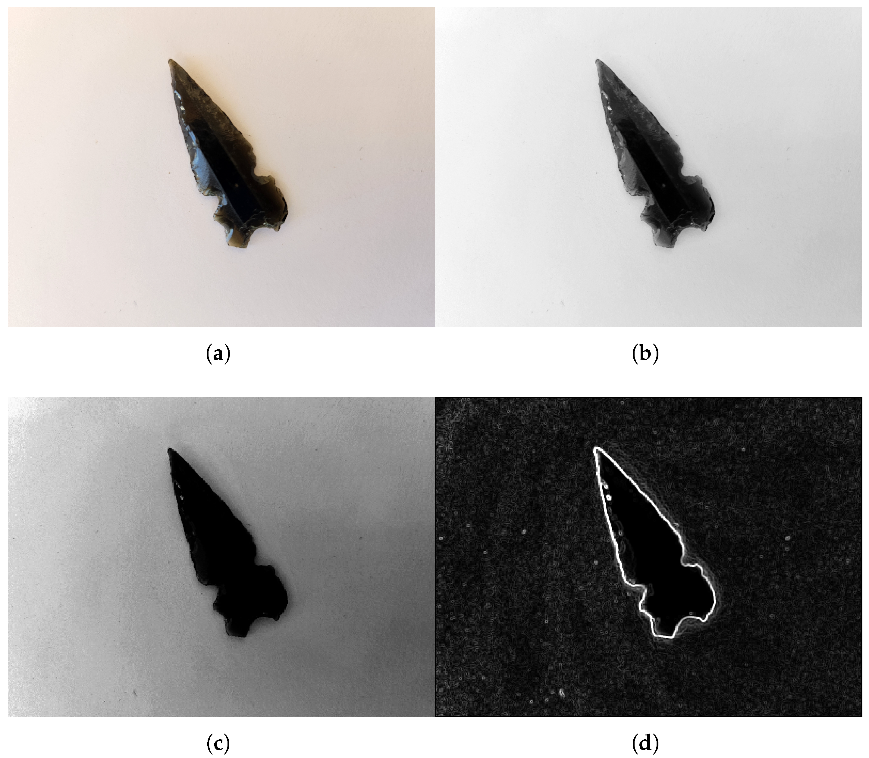
As an example, Figure 2a shows an obsidian arrowhead on a light background. Since the image was acquired at a resolution of $3000\times 4000$ pixels, a reduction process is necessary prior to analysis. Although the contrast facilitates object delineation, the image still presents challenges from residual glare, soft shadows, and contour irregularities, which must be considered in subsequent processing stages.

Figure 2. Image processing sequence: (a) Image of an obsidian arrowhead on white paper, used as $f_0$. (b) The grayscale image ($f_1$) was downscaled to 10% of its original size, resulting in $f_2$. (c) Contrast-enhanced image, denoted as $f_3$. (d) Edges detected using the Sobel operator, denoted as $f_4$.

3.1.2. Extraction of the Color or Intensity Channel

To reduce computational complexity without losing relevant information, a single color or intensity channel is selected. According to Anzueto [17], these channels can be derived from color spaces such as RGB, CMY, YIQ, HSV, or HSI. The selected channel should maximize object-background contrast. The resulting image, denoted as $f_1$, is interpreted as a grayscale matrix defined by the function $f_1:{\mathbb{Z}}^2\to \mathbb{R}$.

3.1.3. Downscaling

Downscaling uniformly reduces the dimensions of $f_1$ to obtain the reduced image $f_2$, preserving the scene’s geometric coherence. This operation—common in both classical processing and deep learning methods—standardizes dimensions and decreases the number of pixels to process. Common techniques include simple sampling, which prioritizes efficiency, and neighborhood averaging, which provides a more stable representation less sensitive to noise (Duque et al. [18]).

3.1.4. Intensity Correction

This stage aims to enhance local and global contrast in the reduced image, generating the corrected image $f_3$, which retains the dimensions of $f_2$. The operation applies an enhancement function to each pixel’s intensity while preserving its spatial position. Among available functions, Klinger [19] highlights the power transformation, whose parameter allows brightening, darkening, or neutralizing the image. In practice, these adjustments facilitate edge detection by reinforcing intensity transitions.

3.1.5. Edge Detection

At this stage, pixels corresponding to object boundaries are identified by evaluating the intensity gradient, producing the set $f_4$. Common methods employ spatial masks such as the Sobel and Prewitt operators (Pajares and De la Cruz [1]). The choice of detector depends on noise level, edge geometry, and scene contrast; this parameter significantly impacts overall performance.

Figure 2b–d illustrate the processing sequence applied to the selected artifact. First, the R channel of the RGB model was extracted due to its lower sensitivity to surface glare compared to the Y channel of YIQ and the V component of HSV. Then, the image was reduced to 10% of its original size using neighborhood averaging, reducing noise and computational load. The final resolution was $300\times 400$ pixels.

Next, contrast correction increased the separation between the object and background, mitigating residual glare effects. Finally, edges were detected using the Sobel operator, which provides stronger responses than the Gradient or Prewitt operators, especially in shadowed areas.

3.1.6. Statistical Thresholding

Edge detection using the operators described generates a two-dimensional matrix indicating pixels with significant intensity variations. Minor changes correspond to uniform regions, while larger variations indicate areas with a high probability of containing edges. In this context, the threshold serves as a boundary distinguishing pixels belonging to edges from those that do not.

In scenarios with controlled lighting and adequate contrast, the threshold can be defined as a constant value. However, under conditions of high variability in acquisition or object characteristics, adaptive methods become necessary.

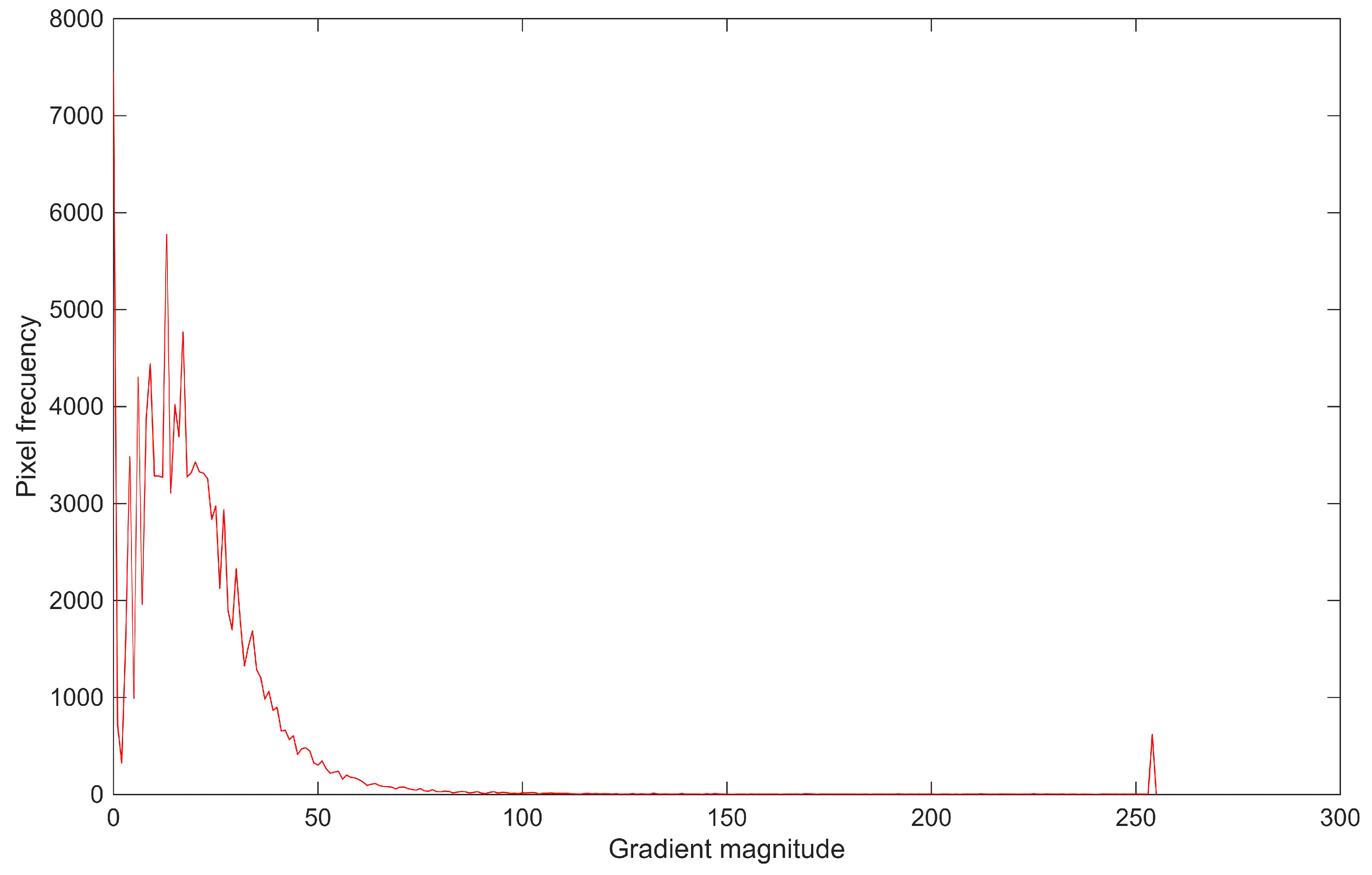
The gradient magnitude histogram, shown in Figure 3, reflects the statistical distribution of intensities. It allows the separation between noise and edges to be identified: the most frequent intensities correspond to minor variations, while higher values—associated with true edges—occur less frequently and are considered atypical.

Figure 3. Histogram of gradient magnitudes in the range 0–255. A high occurrence of low-intensity values, characteristic of noise variations, is observed, in contrast to higher values corresponding to true edges.

Although the gradient distribution is not strictly normal, the standard deviation is used as a robust measure of dispersion. The weighted mean and standard deviation are computed from the histogram using Equations (2) and (3):

$$\mu ={\displaystyle \frac{{\sum }_{i=0}^{255}i·h\left(i\right)}{{\sum }_{i=0}^{255}h\left(i\right)}}$$

(2)

$$\sigma =\sqrt{{\displaystyle \frac{{\sum }_{i=0}^{255}h\left(i\right)·{(i-\mu )}^2}{{\sum }_{i=0}^{255}h\left(i\right)}}}$$

(3)

where

• $\mu$ is the weighted mean of intensity levels.
• $\sigma$ is the standard deviation of intensity levels.
• i is the intensity level (0 to 255 in 8-bit images).
• $h\left(i\right)$ is the absolute frequency of intensity level i.

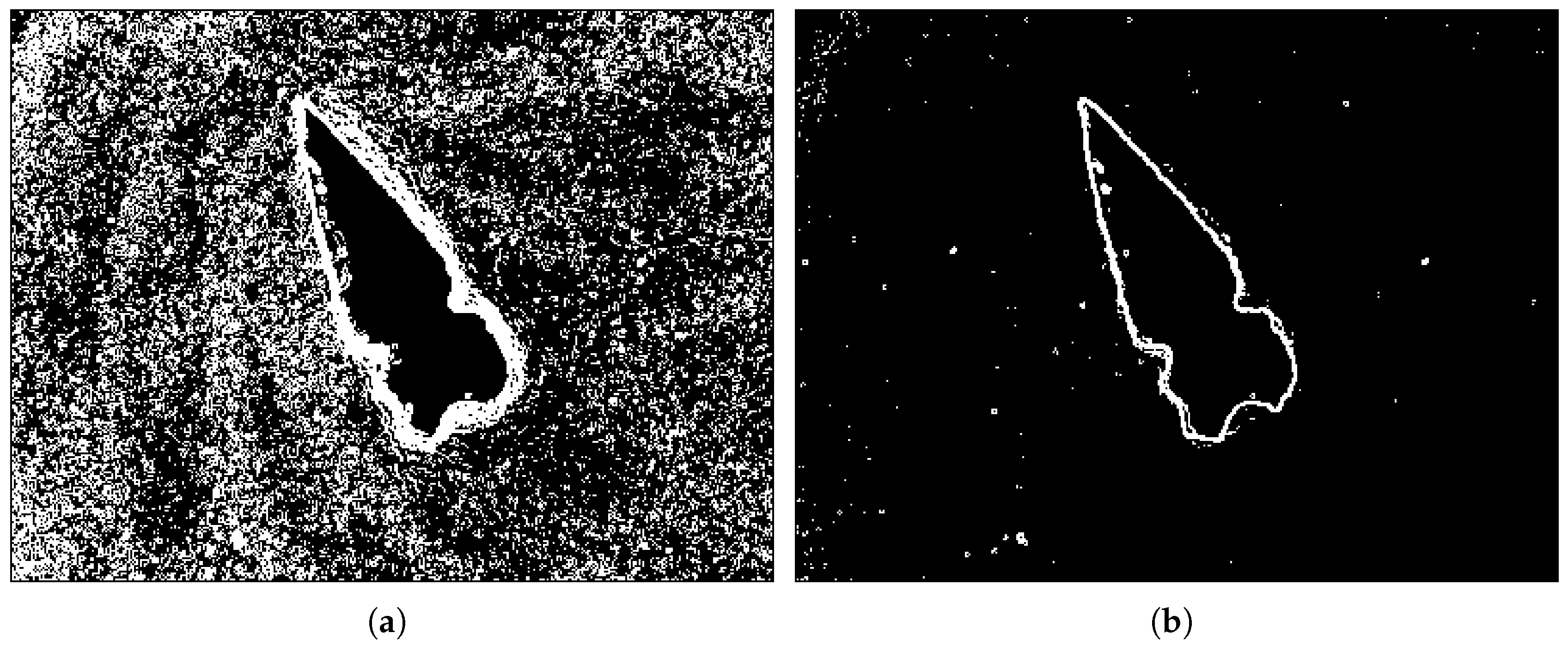
The threshold was defined as three times the standard deviation ($3\sigma$). In approximately normal distributions, this excludes about 0.3% of values at each end, while in non-normal distributions it enables distinction between recurring and atypical data, focusing the analysis on the most significant edges. Figure 4 shows the image $f_4$ being refined as the threshold increases.

Figure 4. Statistical thresholding applied to edge detection: (a) Result using a threshold of one standard deviation ($\sigma$), which preserves approximately one-third of the highest magnitudes, though some noise remains. (b) Result using a threshold of three standard deviations ($3\sigma$), removing most frequent magnitudes while preserving the highest-intensity edges. Some residual noise persists due to glare or surface contamination.

Although different threshold factors—such as $\sigma$ and $2\sigma$—were evaluated, the experimental results indicated that $3\sigma$ provided the most reliable discrimination between noise and true edges. Thresholds below this value preserved a substantial number of responses produced by textured surfaces, shadows, or illumination artifacts, which remained intertwined with the gradient magnitudes of weak edges. By contrast, using $3\sigma$ effectively suppressed these recurring low-magnitude variations while retaining the most prominent responses associated with meaningful boundary structure.

This behavior is consistent with the empirical distribution of gradient magnitudes: the highest values, though infrequent, correspond to spatially coherent alignments that define the object’s contour. As a result, the $3\sigma$ threshold offered a practical compromise, removing the majority of noise without discarding the gradient responses necessary for stable contour characterization. Its selection, therefore, reflects both the statistical properties of the gradient distribution and the observed performance across the complete experimental dataset.

This threshold value is not used to binarize the image, but rather as a reference to compare regions of interest in $f_4$. If no pixel in a region exceeds $3\sigma$, it is considered edge-free and excluded from analysis. Conversely, if higher values are present, these locations are used to characterize the local properties of each region.

3.2. Contour Characterization

Up to this point, the procedure has described the stages of the classical computer vision pipeline that prepare the image and produce the edge map $f_4$, with the aim of linking the detected pixels to form a coherent contour. Although some steps, such as smoothing filtering, have been omitted, the incorporation of additional tools may be considered depending on the specific conditions of the acquisition process. Nevertheless, one of the main objectives of this approach is to minimize the number of operations applied to the image.

At this stage, the analysis is strictly geometric and is restricted to regions of interest, thereby avoiding the need to process the entire image $f_4$ again or to generate additional intermediate representations. This procedure assumes that each selected region contains a single relevant contour, whose characterization can be carried out by sampling the pixels that constitute it.

3.2.1. Region of Interest Extraction

The LRCT procedure is initialized from a user-defined starting point $(x_c,y_c)$ located on, or in the immediate vicinity of, the contour of interest, which defines the center of the first analysis region. Each execution of the algorithm is designed to follow a single contour, and the selection of the initial point determines which contour is characterized. In the presence of multiple objects or contours, the method can be applied independently through separate executions by providing different initial seeds for each contour. In images containing a single dominant contour, the initialization may also be performed automatically by means of a global scan of the image until the first region containing a valid set of edge pixels capable of defining an initial contour segment is identified. Once initialized, the procedure proceeds with a local analysis that requires extracting a square region ${\mathcal{R}}_n$ with side length T pixels—considering T to be odd—and centered at position $(x_c,y_c)$ within the image $f_4$. By design, each analysis region ${\mathcal{R}}_n$ is assumed to contain a single relevant contour segment; scenarios in which multiple contours fall within the same region are outside the scope of the present work and are avoided through appropriate initialization and region sizing.

This region constitutes the minimal unit of analysis in which the enclosed contour segment is assumed to be locally approximated by a linear model. This imposes two requirements: the region must be sufficiently large to describe the local contour direction, while remaining sufficiently constrained to avoid enclosing multiple geometrically distinct sections that would otherwise be associated with a single model.

After the downscaling process described in Section 3.1.3, the images used in this work have a resolution of $400\times 300$ pixels. Since each image contains a single object occupying most of the frame, the region size was selected to be below 10% of the image dimensions while exceeding the minimal $3\times 3$ pixel neighborhood, in order to ensure sufficient support for linear estimation. Under these controlled conditions, values of T in the range of 9 to 15 pixels provided an adequate contour representation while preserving local linearity.

If the highest edge magnitude within ${\mathcal{R}}_n$ is below $3\sigma$, the region is skipped from analysis. Conversely, if two or more pixels exceed this threshold, the characterization process begins by fitting a line to the valid pixels. The line that best represents the contour points within the region is denoted $L_R$.

Figure 5 shows two regions of interest containing a valid contour, used to illustrate the procedure sequence. The region selected on the left side of the shape is denoted ${\mathcal{R}}_1$, while the one on the right side is identified as ${\mathcal{R}}_2$. In both cases, a window size of $T=15$ pixels is considered.

Figure 5. Regions of interest containing a valid contour; the green box indicates the selected search region used for contour tracking.

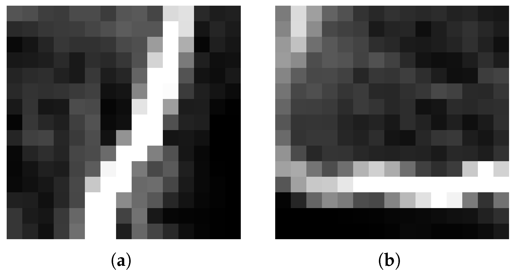
Figure 6 shows the selected regions of interest in detail. In (a) ${\mathcal{R}}_1$ displays a vertically trending edge pointing toward the arrowhead tip, while in (b), ${\mathcal{R}}_2$ exhibits a predominantly horizontal orientation. In both cases, some noise pixels remain despite the previously applied threshold.

Figure 6. Details of the selected regions of interest: (a) Left side of the arrowhead with a predominantly vertical edge trend. (b) Right notch section showing at least two edge directions, although the horizontal orientation predominates.

Once a valid region ${\mathcal{R}}_n$ is extracted from $f_4$, the next step is to locate the edge-descriptor pixels within that region. Each location is evaluated to verify whether its intensity is equal to or greater than $3\sigma$. The coordinates of the valid pixels are stored in the vectors X and Y, as shown in Equation (4).

$$X=\left[\begin{array}{c}{x}_1\\ x_2\\ ⋮\\ x_n\end{array}\right]\mathrm{and}Y=\left[\begin{array}{c}{y}_1\\ y_2\\ ⋮\\ y_n\end{array}\right]$$

(4)

These vectors serve as initial values for line fitting, as some elements may correspond to residual noise. The cleaning process aims to retain only the pixels that can be consistently associated with a line, as detailed in the following sections.

3.2.2. Line Fitting in the Region of Interest

As noted by Chacón et al. [20], in the Cartesian description of a line, there is a difficulty representing steep slopes, since these tend to produce very large values in the intercept. This complicates the mathematical treatment due to the magnitude of the values involved. To overcome this limitation, the polar representation of the line is adopted, expressed in Equation (5).

$$L_R:x\cos \left(\theta \right)+y\sin \left(\theta \right)=\rho$$

(5)

This representation reduces numerical difficulties, as the parameter $\theta$ is bounded, stabilizing the calculation of its values. Similarly, $\rho$ remains within a range comparable to the number of rows or columns of the image, which contributes to stable model handling. It should be noted, however, that multiple equivalent representations can correspond to the same line.

The representation of the region using the thresholded pixels behaves similarly to datasets employed in experimental sciences for fitting models, suggesting that the problem can be addressed using the Least Mean Squares (LMS) method [21]. In this context, the goal is to determine the values of $\theta$ and $\rho$ that best fit the points defined by the position vectors X and Y. For this, the linear system in matrix form shown in Equation (6) is formulated.

$$\left[\begin{array}{cc}X& 1\end{array}\right]\left[\begin{array}{c}-{\displaystyle \frac{\cos \left(\theta \right)}{\sin \left(\theta \right)}}\\ {\displaystyle \frac{\rho }{\sin \left(\theta \right)}}\end{array}\right]=Y$$

(6)

where 1 is a column vector of ones with the same length as X.

Since this system is usually overdetermined, i.e., it has more equations than unknowns, it is multiplied by the transpose of the first factor to obtain a solution using the LMS method [22], as shown in Equation (7).

$${\left(\left[\begin{array}{cc}X& 1\end{array}\right]\right)}^T\left[\begin{array}{cc}X& 1\end{array}\right]\left[\begin{array}{c}-{\displaystyle \frac{\cos \left(\theta \right)}{\sin \left(\theta \right)}}\\ {\displaystyle \frac{\rho }{\sin \left(\theta \right)}}\end{array}\right]={\left(\left[\begin{array}{cc}X& 1\end{array}\right]\right)}^{T}Y$$

(7)

Solving this system allows obtaining the parameters required to calculate $\theta$ and $\rho$, which define the characteristic line of the local edge. However, it is observed that while the fit is adequate for predominantly horizontal lines, it loses precision for predominantly vertical orientations. This is because the LMS algorithm minimizes vertical errors, making it more effective for the first case, where the vertical positions of the points vary more uniformly. In contrast, for near-vertical lines, this strategy tends to produce inaccurate results.

Rotation of the Region of Interest

An effective solution is to apply a temporary rotation of the region with respect to the Cartesian origin of the image. This procedure swaps the reference axes so that the points along the horizontal axis are reassigned to the vertical axis and vice versa, following the relation $X_r=-Y$ and $Y_r=X$, where $X_r$ and $Y_r$ are the transformed vectors introduced into the LMS procedure. This way, a vertically trending line can be evaluated as if it were horizontal. Subsequently, the obtained $\theta$ is corrected by subtracting ${\displaystyle \frac{\pi }{2}}$ to compensate for the rotation and restore the orientation in the original system, while $\rho$ remains unchanged, as it represents the perpendicular distance from the line to the origin, which is unaffected by this transformation.

Therefore, it is advisable to perform both fits using the LMS algorithm, considering the possibility that the image contains edges with both horizontal and vertical orientations.

Applying this approach yields two possible line descriptions. One way to select the best approximation is by using the coefficient of determination $R^2$, as used by Purri and Dana [23], expressed in Equation (8).

$$R^2=1-{\displaystyle \frac{\sum {(y_i-{\widehat{y}}_i)}^2}{\sum {(y_i-\overline{y})}^2}}$$

(8)

where

• $y_i$ are the original values of the thresholded pixels, i.e., elements of the vector Y.
• ${\widehat{y}}_i$ are the values predicted by the line, calculated from the parameters $\theta$ and $\rho$ obtained in the fit.
• $\overline{y}$ is the mean of the values in vector Y.

This coefficient allows assessing how representative the obtained line is with respect to the detected edge points in the analyzed region. An $R^2$ value close to 1 indicates a reliable fit, while values near 0 suggest that the line does not adequately describe the data.

The coefficient should be calculated for both cases—rotated and unrotated—and evaluated according to vectors Y or $Y_r$. The highest $R^2$ value determines the parameters corresponding to the best approximation of the characteristic line.

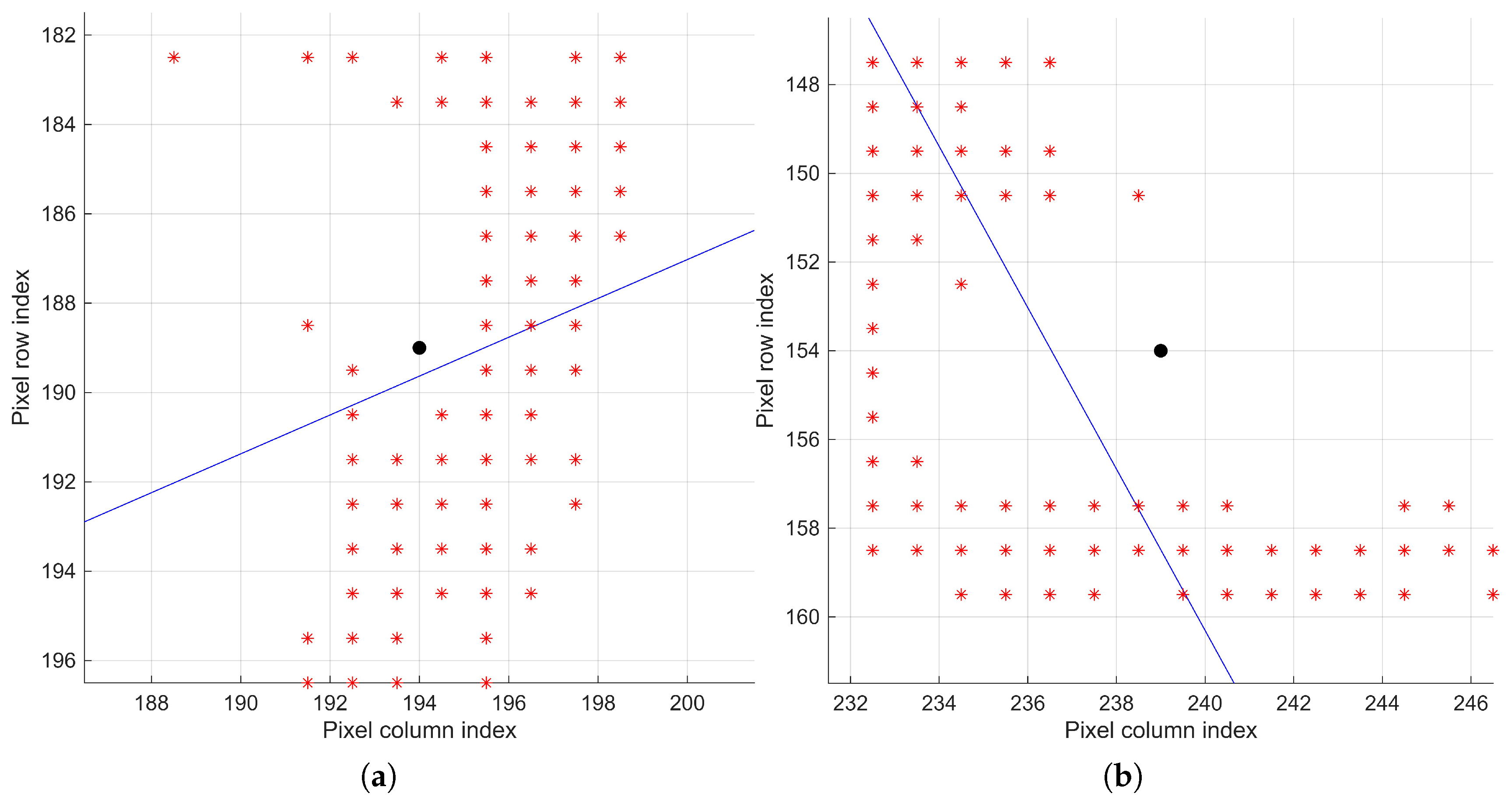
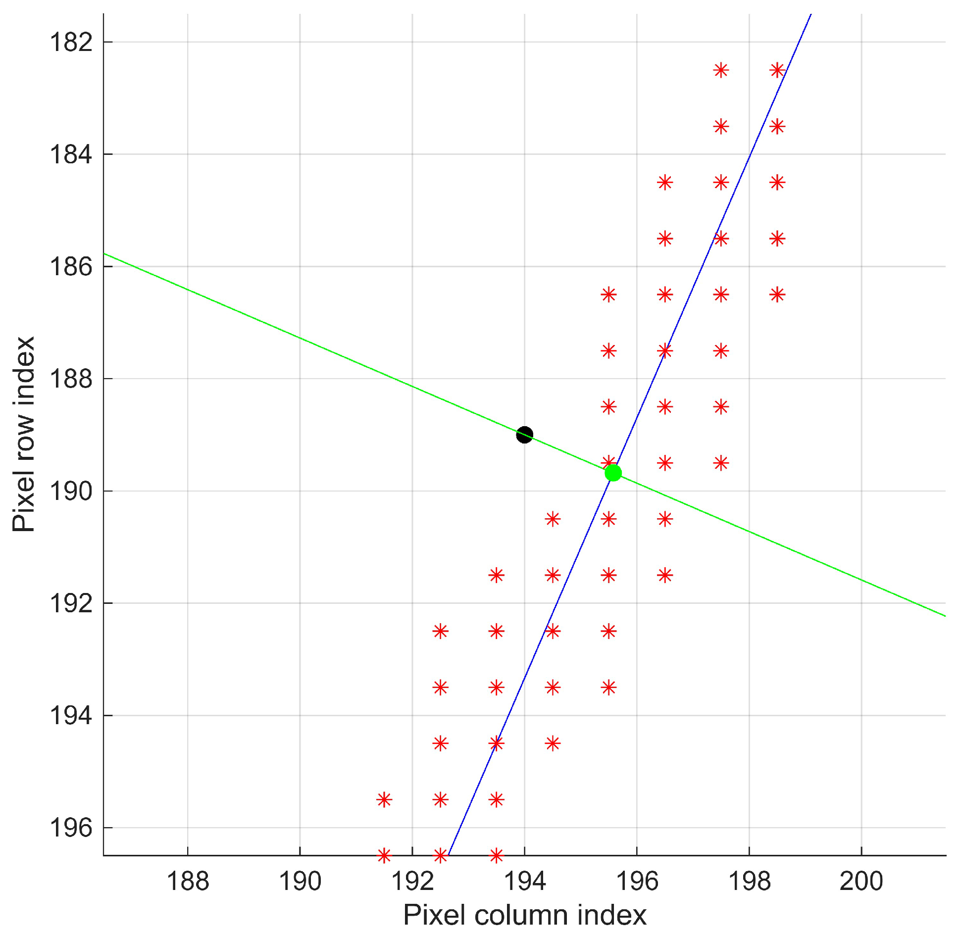
Figure 7 shows the line fitting for regions ${\mathcal{R}}_1$ and ${\mathcal{R}}_2$, illustrating the initial linear approximation to the edge pixels. As can be observed, the fitted lines account for the positions of all valid pixels, although they do not accurately describe the local continuity trend when noise pixels are present or when the analysis is near a contour direction change point.

Figure 7. Line fitting obtained for regions (a) ${\mathcal{R}}_1$ and (b) ${\mathcal{R}}_2$. Lines $L_1$ and $L_2$ (blue) represent the linear model fitted to the edge pixels (red asterisks *), while the black dot indicates the geometric center of each region.

On the Use of LMS and Alternative Fitting Methods

It is worth noting that more general line-fitting alternatives exist, such as the Total Least Squares (TLS) method, which minimizes the error perpendicular to the line and is therefore inherently rotation invariant. However, within the geometric framework of LRCT, the regions ${\mathcal{R}}_n$ contain small local sets of highly collinear points, where residual noise originates primarily from variations in gradient magnitude and produces a dominant dispersion along a single direction. Under these conditions, the use of LMS combined with the temporary rotation yields numerically stable behavior at a lower computational cost than TLS, which typically requires a singular value decomposition (SVD). Moreover, the proposed scheme enables explicit control over the quality of the fit through the coefficient $R^2$, which aligns with the lightweight and transparent design goals of LRCT. Nevertheless, the exploration of TLS in its standard two-dimensional formulation remains a promising direction for future work, particularly for scenarios involving more symmetric noise or greater variability in local edge orientation.

Correction of Deviations in Linear Fitting

Since the LMS method considers both points belonging to true edges and those affected by noise, the procedure is iterated by removing from vectors X and Y the point with the greatest distance from the fitted line. This distance is calculated as follows:

$$d_r=\left|x_n\cos \left(\theta \right)+y_n\sin \left(\theta \right)-\rho \right|$$

(9)

From the set of distances obtained, the maximum value is identified. If this distance exceeds two pixels, the corresponding point is removed from the vectors, and the fitting is repeated. This process continues until all remaining points lie on the line or within a tolerable neighborhood, achieving a more robust fit against noise.

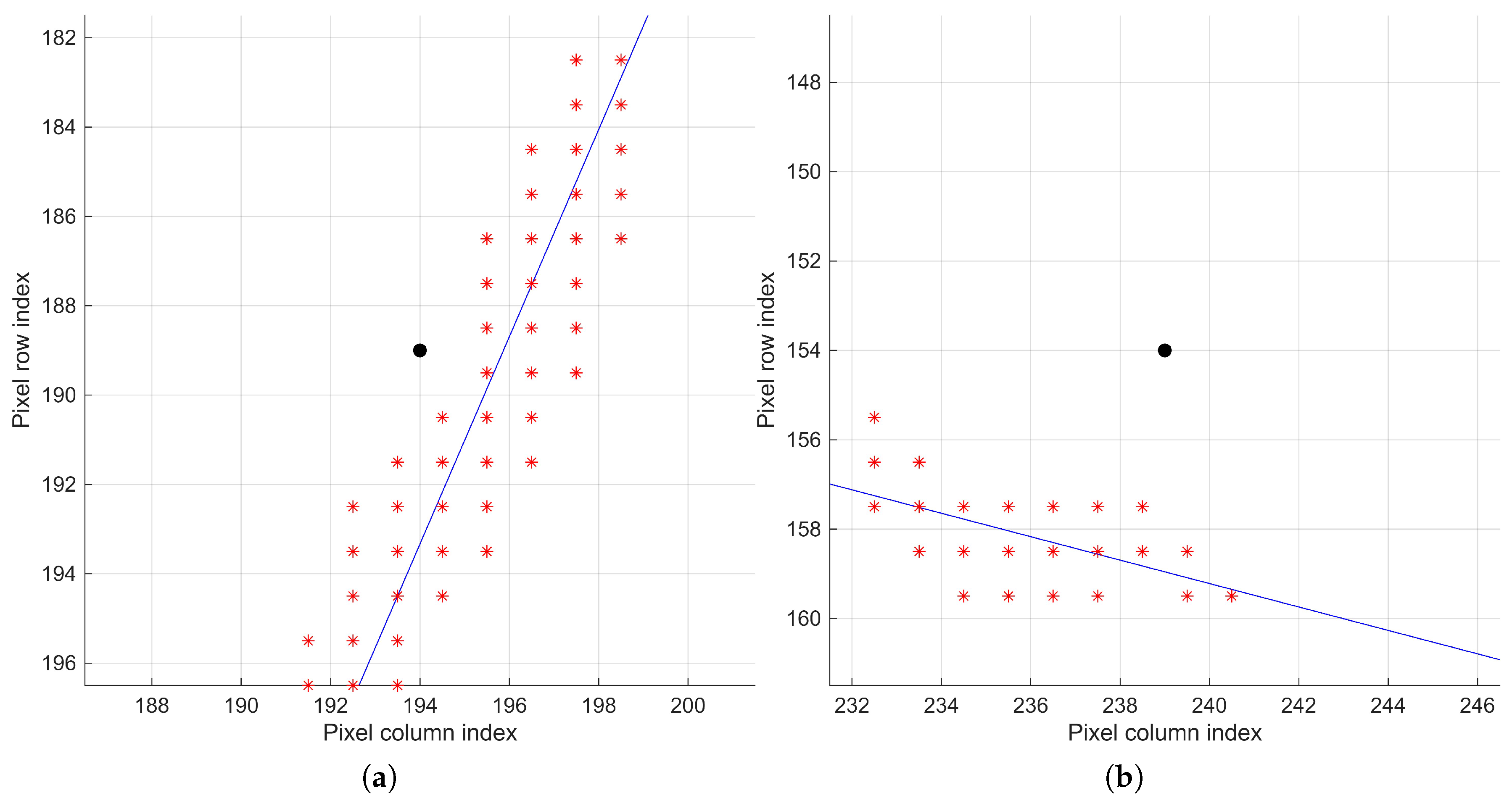
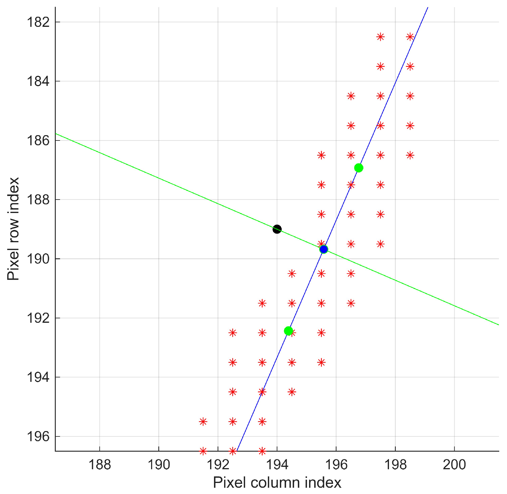
Figure 8 shows the final versions of lines $L_1$ and $L_2$ for regions ${\mathcal{R}}_1$ and ${\mathcal{R}}_2$ after iteratively removing the most distant points. The lines approximate areas with the highest pixel density, treating the farthest elements as noise.

Figure 8. Final line fitting after iterative removal of noisy pixels in the regions of interest (a) ${\mathcal{R}}_1$ and (b) ${\mathcal{R}}_2$. A better correspondence between the fitted line and the remaining edge pixels (shown as red asterisks*) is observed; the black dot denotes the geometric center of each region.

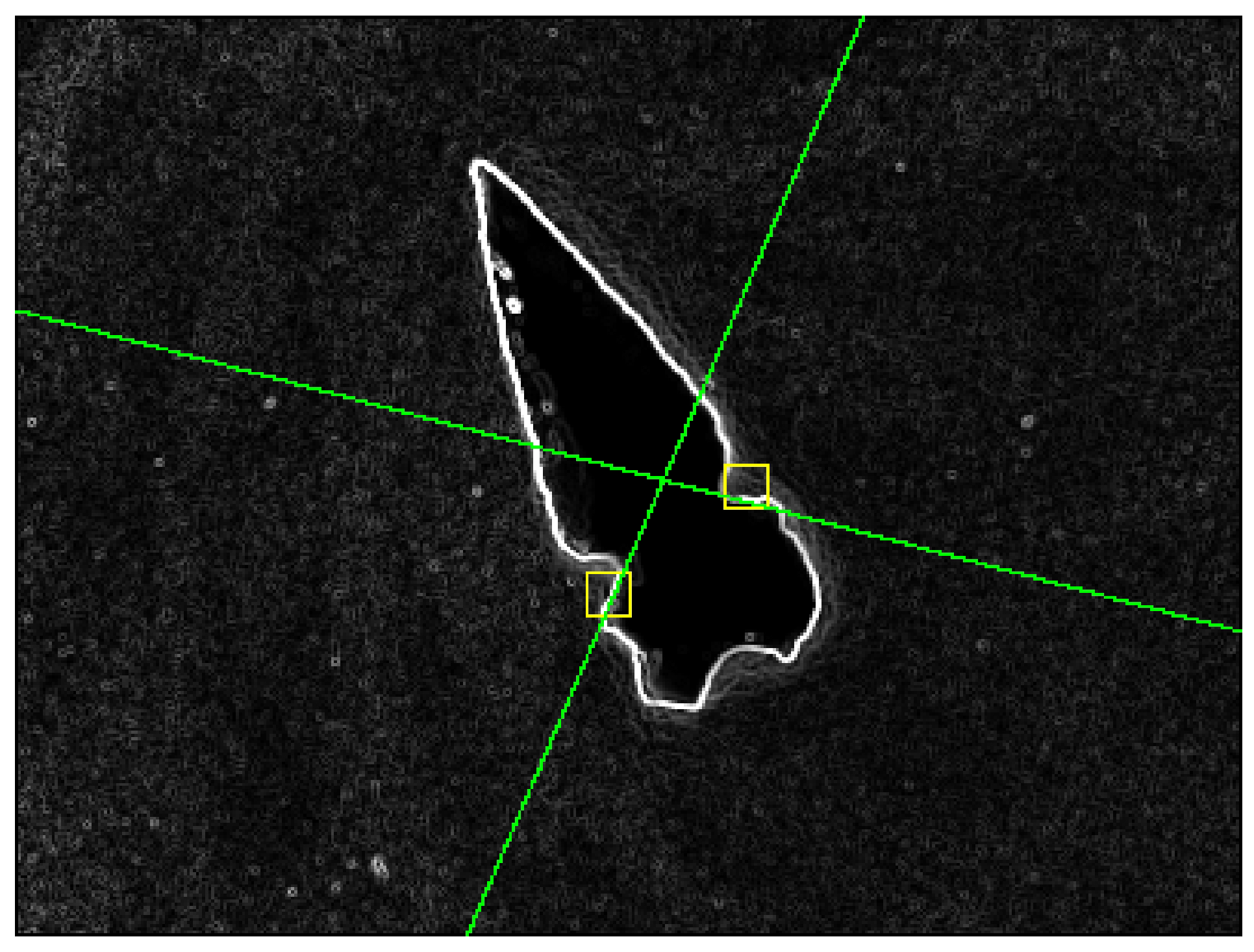
At this stage, it can be observed that a proper prior image acquisition and processing procedure not only increases the contour accuracy but also reduces the number of iterations needed for an adequate description. Figure 9 shows the lines extended over image $f_4$, demonstrating that the procedure approximates the lines tangentially along the contour, sufficient to estimate the location of the next analysis region.

Figure 9. Lines $L_1$ and $L_2$ obtained for regions ${\mathcal{R}}_1$ and ${\mathcal{R}}_2$, overlaid on image $f_4$. Locally, these lines approximate an instantaneous tangent of the contour; the yellow box indicates the local region of interest used for line estimation.

3.2.3. Contour Points

At this stage, the procedure defines how points representing the object’s contour are selected from the search regions ${\mathcal{R}}_n$. It is important to clarify that the point $(x_c,y_c)$ corresponds to the center of region ${\mathcal{R}}_n$ and does not necessarily lie on the representative line $L_n$. For this reason, $(x_c,y_c)$ is used only as a reference to locate the next analysis region and not as a contour point itself.

To record a point that belongs to the contour, $(x_r,y_r)$ is identified, which lies on the line $L_n$ and maintains geometric proximity to the region center $(x_c,y_c)$. This procedure is illustrated in Figure 10, showing the relationship between $(x_c,y_c)$ and $(x_r,y_r)$ in region ${\mathcal{R}}_1$.

Figure 10. Geometric relationship between the region center $(x_c,y_c)$ and the contour point $(x_r,y_r)$ in region ${\mathcal{R}}_1$. The region center is shown as a black dot, the contour point as a green dot, and the remaining edge pixels are represented by red asterisks (*). The line $L_1$ (blue) corresponds to the fitted contour line, while the perpendicular line $L_P$ (green) connects $(x_c,y_c)$ and $(x_r,y_r)$.

Graphically, $(x_r,y_r)$ corresponds to the intersection point between the line $L_n$ and its perpendicular $L_P$, defined as

$$x\cos \left({\theta }_P\right)+y\sin \left({\theta }_P\right)={\rho }_P,$$

where $L_P$ passes through the region center $(x_c,y_c)$. The parameters ${\theta }_P$ and ${\rho }_P$ are calculated as

$${\theta }_P=\theta +{\displaystyle \frac{\pi }{2}},{\rho }_P=x_c\cos \left({\theta }_P\right)+y_c\sin \left({\theta }_P\right)$$

(10)

The contour point is approximated using the following expressions:

$$x_r={\displaystyle \frac{\rho \sin \left({\theta }_P\right)-{\rho }_P\sin \left(\theta \right)}{\sin \left({\theta }_P\right)\cos \left(\theta \right)-\sin \left(\theta \right)\cos \left({\theta }_P\right)}},y_r={\displaystyle \frac{\rho -x_r\cos \left(\theta \right)}{\sin \left(\theta \right)}}$$

(11)

This procedure ensures that the analysis regions remain close to the actual contour, iteratively adjusting the center toward areas with effective edges and recording each identified contour point.

3.2.4. Search Directions and Contour Tracking

Contour tracking is based on a geometric model inspired by human visual attention, progressing from an initial point until reaching a stopping boundary or returning to the starting point in closed contours.

After characterizing a region, it is necessary to define a new reference point from which the tracking process is re-evaluated. In the proposed approach, a new search region is placed at a distance $d_b$, expressed in pixels from point $(x_r,y_r)$, and displaced along the line estimated in the previous iteration.

A minimal search distance of one pixel could generate an overly dense sequence of edge pixels; although this alternative may seem appropriate, it significantly increases the number of operations and, consequently, the computational cost. In contrast, an excessively large value of $d_b$ may cause the subsequent region ${\mathcal{R}}_n$ to deviate from the contour, thus compromising tracking continuity.

To ensure tracking continuity, it is essential to guarantee overlap between adjacent search regions so that common pixels are analyzed in consecutive iterations and lines with consistent geometric characteristics are obtained. For this reason, the next search point is required to remain within the current analysis region, a condition satisfied by enforcing $d_b<T/2$, which preserves the geometric coherence of the tracking process.

As can be observed, the parameters T and $d_b$ must be selected jointly, since they control both the size of the analysis area during tracking and its displacement along the contour. Contours with low geometric complexity allow the use of larger values of T and $d_b$, whereas more irregular geometries or those with local changes in direction require smaller analysis regions and shorter search displacements. This selection should be adapted to the image resolution and to the scale of the contour: in higher-resolution images, larger values of T can be employed to preserve the validity of the local linear approximation, with $d_b$ adjusted accordingly, while in lower-resolution images or in contours with fine irregularities, smaller values of both parameters are preferable to maintain tracking coherence and control computational cost.

For each point $(x_r,y_r)$, two possible centers for the next region are defined, $(x_{b1},y_{b1})$ and $(x_{b2},y_{b2})$, located at a distance $d_b$ along the line $L_n$, as illustrated in Figure 11. These search centers are given by:

$$x_{b1}=x_c-d_b\sin \left(\theta \right),y_{b1}=y_c+d_b\cos \left(\theta \right)$$

(12)

$$x_{b2}=x_c+d_b\sin \left(\theta \right),y_{b2}=y_c-d_b\cos \left(\theta \right)$$

(13)

Figure 11. Search points $(x_{b1},y_{b1})$ and $(x_{b2},y_{b2})$ (green) adjacent to the contour point $(x_r,y_r)$ (blue) in region ${\mathcal{R}}_1$, with $d_b=3$ pixels. The remaining edge pixels are represented by red asterisks (*), and the black dot indicates the geometric center of the region.

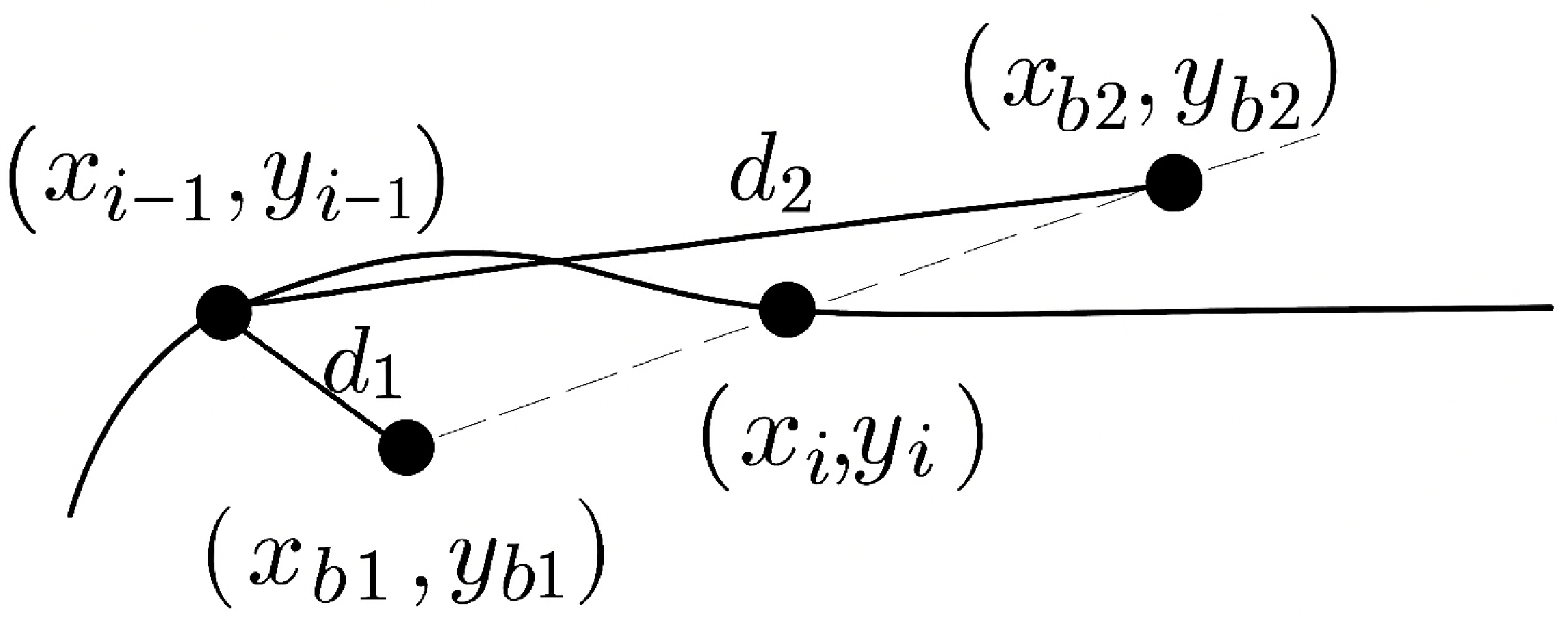
Complete contour tracking requires iterating this procedure over a sequence of regions ${\mathcal{R}}_i$. Each point $(x_{r,i},y_{r,i})$ generates two possible collinear continuations: $(x_{b1,i},y_{b1,i})$ and $(x_{b2,i},y_{b2,i})$. The option selected is the one farthest from the previous position $(x_{r,i-1},y_{r,i-1})$, assuming that contour transitions are smooth. This selection procedure is illustrated in Figure 12.

Figure 12. Selection of the new region center $(x_{r,i+1},y_{r,i+1})$ based on the current $(x_{r,i},y_{r,i})$ and previous $(x_{r,i-1},y_{r,i-1})$ positions. The farthest option between $(x_{b1,i},y_{b1,i})$ and $(x_{b2,i},y_{b2,i})$ is chosen to continue contour tracking.

The corresponding distances are calculated according to Equations (14) and (15):

$$d_1=\sqrt{{(x_{r,i-1}-x_{b1,i})}^2+{(y_{r,i-1}-y_{b1,i})}^2}$$

(14)

$$d_2=\sqrt{{(x_{r,i-1}-x_{b2,i})}^2+{(y_{r,i-1}-y_{b2,i})}^2}$$

(15)

The point associated with the greatest distance determines the center of the next region, $(x_{r,i+1},y_{r,i+1})$.

Stopping Condition

For closed contours, the distance between $(x_{r,i+1},y_{r,i+1})$ and the initial point $(x_0,y_0)$ is calculated. If this distance is less than or equal to $d_b$, the contour traversal is considered complete.

Upon closing the path, the initial value $(x_{-1},y_{-1})$ is discarded, as it does not belong to the contour and was only used to determine the search direction. The remaining points form the contour sampling, represented by the arrays $X_b$ and $Y_b$. Plotting them in XY format reconstructs the shape of the object.

3.3. Result Presentation

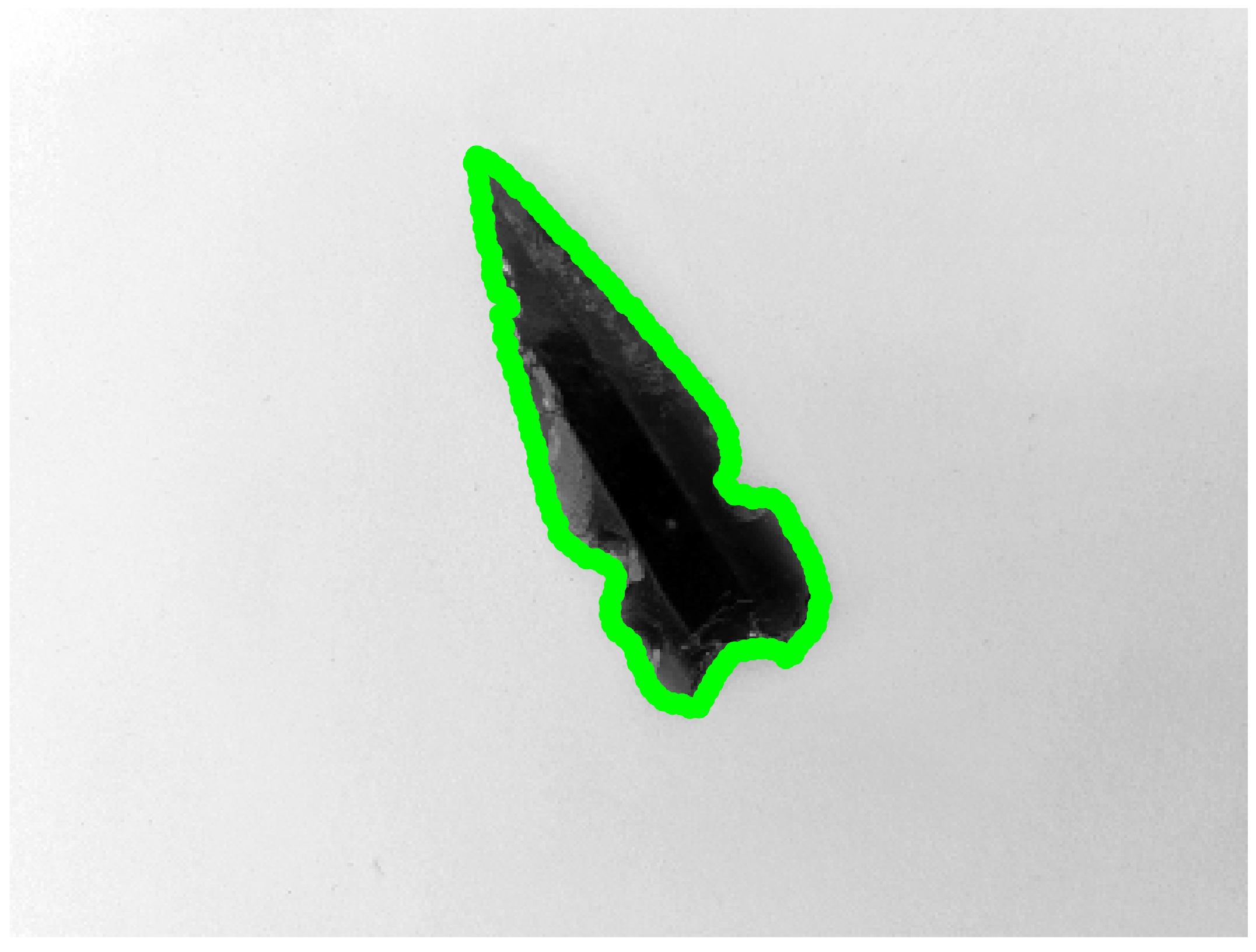
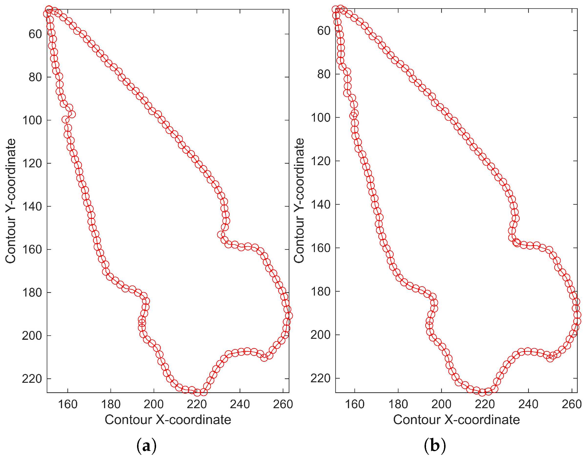
Applying the procedure with a region size of $T=15$ pixels, a search distance of $d_b=3$ pixels, and starting from the section previously designated as ${\mathcal{R}}_1$, allowed us to obtain the contour correspondence $(x_{r,i},y_{r,i})$ shown in Figure 13, consisting of a total of 160 points.

Figure 13. Results of chaining the contour pixels $(x_{r,i},y_{r,i})$, superimposed on the original image. Although the chaining is adequate, the brightness condition present in the initial environment locally influenced the contour-search trajectory.

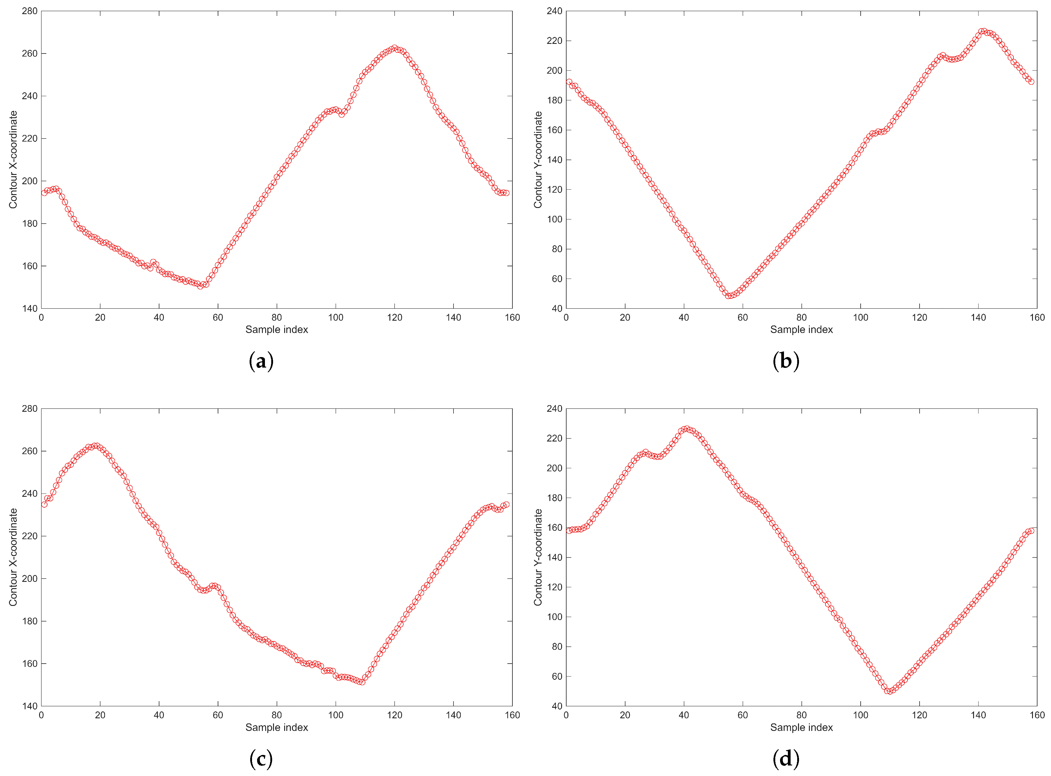
As observed in Figure 14, when comparing the chains obtained by starting in regions ${\mathcal{R}}_1$ and ${\mathcal{R}}_2$, the resulting sets are not identical; that is, the procedure is not invariant to the same shape. This occurs because the starting point determines the sampling sequence. Thus, even when maintaining the same search direction, the signals exhibit a phase shift as well as slight variations in magnitude for the same region.

Figure 14. Chains produced under identical image-processing and contour-search conditions, but with starting points located in (a) ${\mathcal{R}}_1$ and (b) ${\mathcal{R}}_2$. A high similarity between both contours is observed, although differences arise in the manner each one traverses the region affected by brightness noise.

Additionally, the search direction plays a decisive role. When opposite trajectories are followed, the $X_b$ and $Y_b$ components reverse their sampling order, even though the X–Y plot retains the same appearance. In this case, regions ${\mathcal{R}}_1$ and ${\mathcal{R}}_2$ produced opposite search directions, resulting in inverted and phase-shifted sequences, as illustrated in Figure 15.

Figure 15. Breakdown of the $X_b$ and $Y_b$ components for (a,b) ${\mathcal{R}}_1$ and (c,d) ${\mathcal{R}}_2$. Although the magnitude differences are small, the components exhibit a phase shift due to the choice of different starting points and appear rotated along the sample index as a consequence of the opposite search directions.

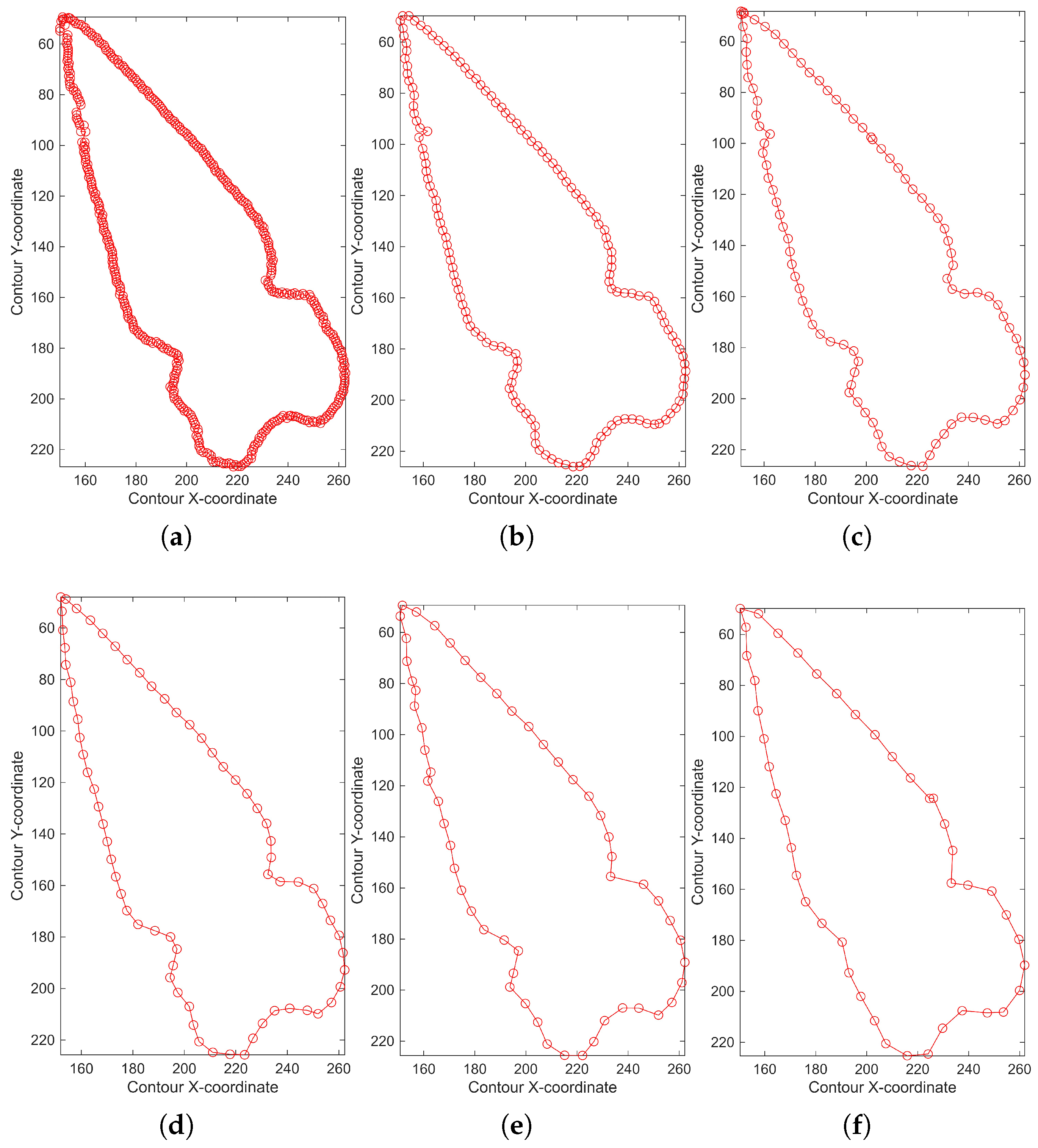
Finally, it was observed that the parameter $d_b$ directly influences the sampling density and the number of points defining the contour. Small values of $d_b$ produce denser and more detailed trajectories, yielding more precise contour chaining at the expense of increased computational cost. Conversely, larger values reduce the number of operations but degrade the descriptive quality by omitting fine geometric details. As illustrated in Figure 16, increasing $d_b$ progressively simplifies the contour while preserving its overall shape. In the extreme case of $d_b=11$, it was necessary to increase the search region size to $T=21$ pixels in order to maintain tracking continuity. These results support the design choice that $d_b$ should remain below half of T. This behavior confirms the inverse relationship between spatial sampling resolution and the efficiency of the contour-chain representation.

Figure 16. Contour samplings obtained from the same image-processing routine, starting at region ${\mathcal{R}}_1$ and with $T=15$ pixels, for different values of the parameter $d_b$. Panels (a–f) show the results for $d_b=1,3,5,7,9,$ and 11 pixels, respectively, demonstrating the progressive reduction in the number of points and level of detail as the sampling separation increases.

In summary, although the resulting contour analysis may vary depending on the starting point or the spacing between evaluation regions, the data can be treated as a discrete signal. This makes them suitable for processing using techniques such as correlation, convolution, or the discrete Fourier transform, where the emphasis lies on the global description and chaining of the contour rather than on the internal organization of the data.

4. Results

Since this study is intended to support the analysis of archaeological materials—where the morphology of objects serves as a fundamental descriptor for inferring manufacturing processes, use, and provenance—twelve representative pieces were selected from different materials and industries commonly found in archaeological contexts. The sample includes replicas of obsidian arrowheads representing the lithic industry, ceramic fragments associated with pottery, as well as shell and bone pieces corresponding to malacological and osseous industries, respectively. This selection enables the method to be evaluated across surfaces, textures, and geometries comparable to those encountered in real archaeological contexts.

In addition, modern manufactured objects made of metal and characterized by predominantly rectilinear geometries were incorporated to analyze the performance of the method in the presence of abrupt discontinuities along the contour.

The experimental tests were carried out on a system running Windows 11, equipped with an AMD Ryzen 7 7435HS processor and 24 GB of RAM. All algorithms were executed on the CPU without GPU acceleration. The development environment was MATLAB R2024b.

As no equivalent algorithm exists that receives a preprocessed image as input and directly produces organized contour coordinates, the results produced by LRCT were compared against edges obtained using the Canny algorithm [5] complemented with Moore–Neighbor tracing [6]. Hereafter, this combination of procedures is referred to jointly as Canny+Moore.

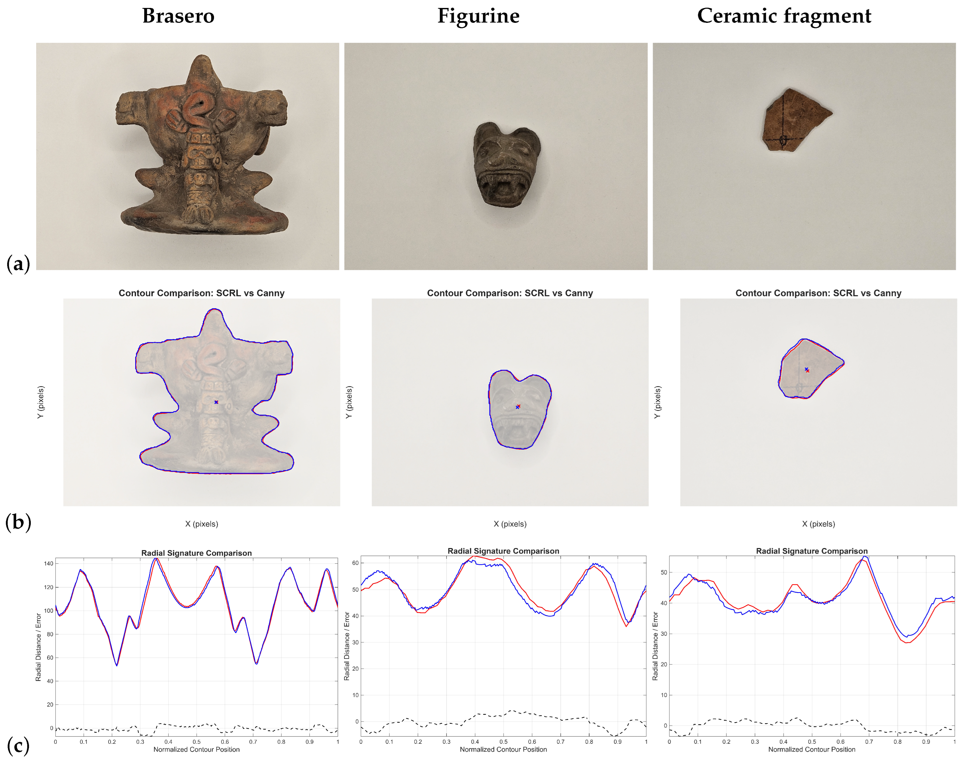
For the qualitative analysis, contours generated by both methods were obtained from the same input image. By overlaying their respective $XY$ coordinates on the original image, it is possible to directly observe both their correspondence and the discrepancies that arise between them.

Subsequently, the centroid of each point set was computed to generate the radial signature, defined as the distance from each contour point to the centroid. The comparative analysis of the radial signals obtained from both methods quantifies their differences and provides an estimate of the error between procedures.

The tables and figures illustrating these results are organized by material category: ceramics (Figure 17), obsidian lithics (Figure 18), bone (Figure 19), metal objects (Figure 20), and shell (Figure 21).

Figure 17. Comparison between LRCT and Canny+Moore applied to three ceramic elements: (a) original image; (b) detected contours (red: LRCT, blue: Canny+Moore); (c) radial signatures and differences between curves (black dashed line). This case evaluates performance under irregular shapes and tonal variations characteristic of pottery, one of the most abundant archaeological materials.

Figure 18. Comparison between LRCT and Canny+Moore applied to obsidian pieces: (a) original image; (c) radial signatures and curve differences. (b) detected contours (red: LRCT, blue: Canny+Moore); Obsidian, with its high reflectance and sharp edges, poses a challenge for conventional edge detectors.

Figure 19. Comparison between LRCT and Canny+Moore applied to bone fragments: (a) original image; (b) detected contours (red: LRCT, blue: Canny+Moore); (c) radial signatures and curve differences. Bone presents naturally nonlinear geometries, useful for evaluating method stability along smooth edges.

Figure 20. Comparison between LRCT and Canny+Moore applied to metallic objects: (a) original image; (b) detected contours (red: LRCT, blue: Canny+Moore); (c) radial signatures and curve differences. The evaluation focuses on straight contours and abrupt direction changes.

Figure 21. Comparison between LRCT and Canny+Moore applied to shell elements: (a) original image; (b) detected contours (red: LRCT, blue: Canny+Moore); (c) radial signatures and curve differences. These cases assess performance under irregular edges with undulations and zigzag patterns.

For the quantitative analysis, minimum but sufficient values of T and $d_b$ were established to ensure the successful processing of each contour. Both methods were then executed, recording the processing time in milliseconds as an indicator of computational cost, as well as the number of samples obtained in each case. Additionally, the average error between radial signatures and the maximum observed error were computed as comparative metrics of similarity between the two results. For the fifteen selected objects, the data are presented in Table 1.

Table 1. Quantitative comparison between the Canny+Moore algorithm and the LRCT method. The table reports the LRCT parameter settings, the number of samples obtained, the average and maximum errors between radial signatures, and the execution times.

Object	T (px)	${\mathit{d}}_{\mathit{b}}$ (px)	Canny Samples	LRCT Samples	Mean Error (px)	Max. Error (px)	Canny Time (ms)	LRCT Time (ms)
Brasero	11	3	983	351	2.40	6.90	57	133
Figurine	11	5	323	72	2.70	6.30	61	58
Ceramic fragment	11	5	240	59	2.90	6.00	86	73
Arrowhead 1	11	2	429	235	3.20	9.30	54	294
Arrowhead 2	11	2	673	357	4.40	9.50	54	124
Arrowhead 3	11	2	615	327	2.80	7.10	70	146
Bone 1	11	5	1020	234	5.80	11.30	76	95
Bone 2	11	7	1190	188	5.20	12.00	75	136
Bone 3	11	5	455	103	4.20	11.80	64	94
Nut	11	2	246	133	2.20	4.70	59	71
Triangle	11	2	210	117	1.80	5.00	54	68
Hex key	11	3	563	239	2.80	6.60	73	112
Shell 1	11	7	280	49	2.90	3.90	66	52
Shell 2	9	2	482	271	0.80	2.89	196	87
Shell 3	9	2	518	292	9.40	21.00	55	100

The results indicate that the LRCT method produces a substantially smaller number of contour points, achieving reductions ranging from 43% to 84% relative to the points generated by Canny+Moore. On average, LRCT eliminates approximately 61% of the samples and, in the most representative cases, describes the contour using only 15–30% of the points.

Since the qualitative comparisons show that the contours remain consistent for all elements (see Figure 19), it can be affirmed that LRCT produces compact and descriptive representations suitable for subsequent analysis of the contour as a discrete signal.

The method controls its sampling resolution through the search distance $d_b$, which must be chosen in accordance with the region size T. Its defining characteristic is the organized sampling of the contour via sequential tracking based on regions of interest. A larger $d_b$ results in fewer samples, while a smaller value increases sample density.

The average error remains within a range of 2–4% of the pixel dimensions. Excluding the outlier of 21 px, maximum deviations reach approximately 12 px, likely associated with the displacement of the region of interest caused by noise or limited edge sharpness. These errors are acceptable considering the image resolution of $400\times 300$ px.

Although Canny+Moore yields shorter execution times, LRCT can approach comparable speeds by reducing the number of generated samples, indicating that efficiency depends on both the tracking algorithm and the required number of samples.

In the $XY$ representations, the contours generated by both methods correspond to the outer boundary of the objects. Because conventional edge detectors may be ambiguous, a contour is considered adequate if it remains close to the object’s periphery and does not invade background or interior regions.

In all cases, the centroids estimated by both methods were located very close to each other, and the radial signatures exhibited similar overall shapes, confirming the geometric correspondence of the results.

In the ceramic series (Figure 17), both methods generate contours consistent with the object’s geometry. However, Canny+Moore exhibits stepped or zigzag segments, especially in regions of high curvature. In contrast, LRCT produces a smoother and more stable trace due to its regional analysis, which selects representative points based on local neighborhoods.

This difference is reflected in the radial signatures, where LRCT curves exhibit fewer fluctuations and a more consistent global shape, particularly in small objects.

Taken together, these results indicate that LRCT reduces the number of required samples while improving geometric continuity.

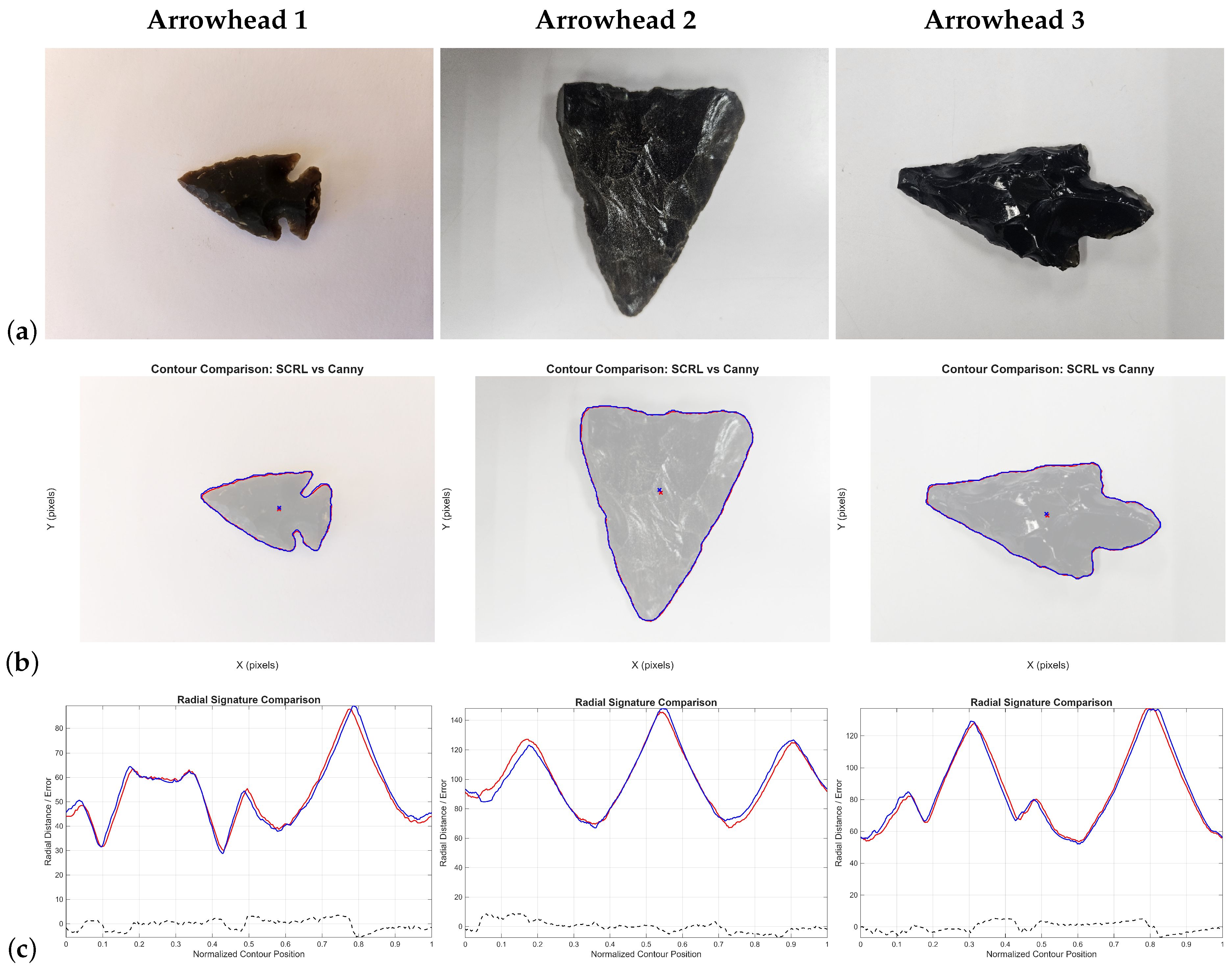
For lithic materials (Figure 18), preprocessing was critical due to internal edges and specular reflections. After contrast enhancement, both methods generated congruent contours, although slight displacements appear in the radial signatures. Canny+Moore exhibited stepping, whereas LRCT maintained a smoother and more stable boundary.

In several tests for Arrowhead 1, the LRCT algorithm temporarily interpreted an internal contour as part of the external boundary, which produced an abrupt jump in the radial signature. This behavior was later corrected by adjusting the parameters used to define the analysis region.

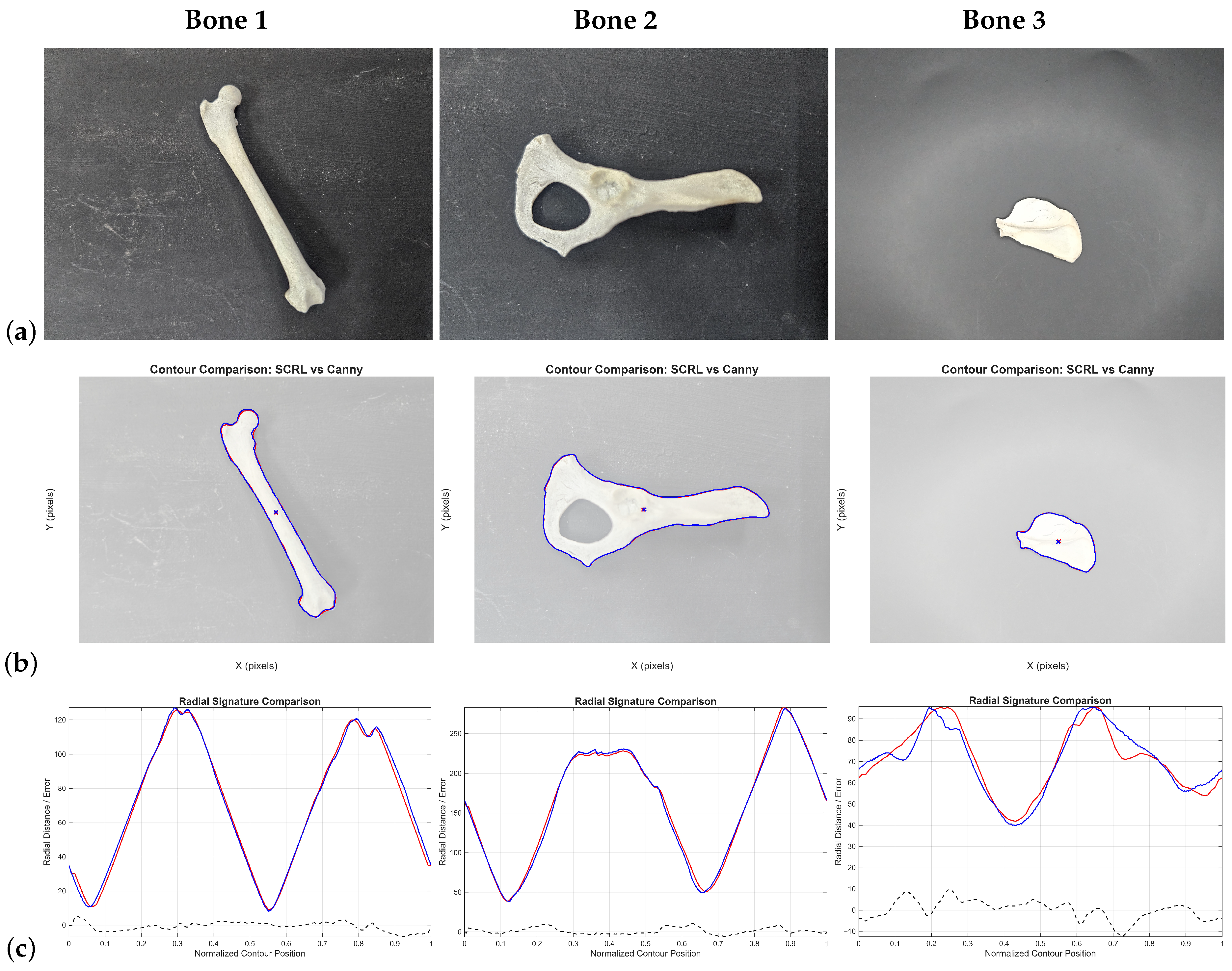
In the bone samples, both methods produced correct contours, although Canny+Moore exhibited implausible discontinuities due to the small object size relative to the image. LRCT maintained greater contour stability. Increasing object–background contrast was necessary to preserve edges.

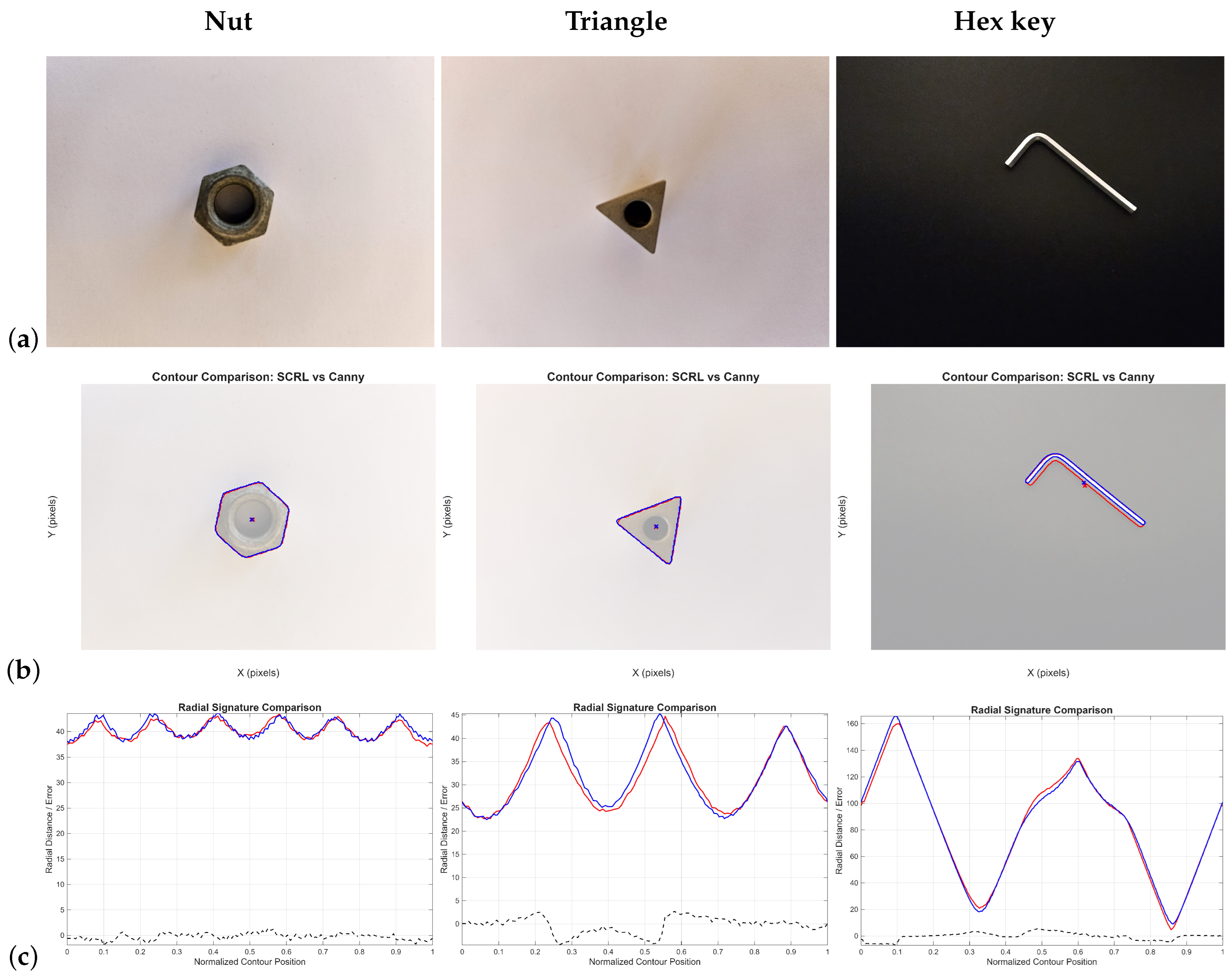
For metallic objects, both methods exhibit stepping in edges, although LRCT does so to a lesser extent. This arises from the discrete nature of raster images, where perfectly straight edges are difficult to represent. In the Hex key, LRCT followed the outer boundary more accurately, while Canny+Moore shifted toward an internal contour.

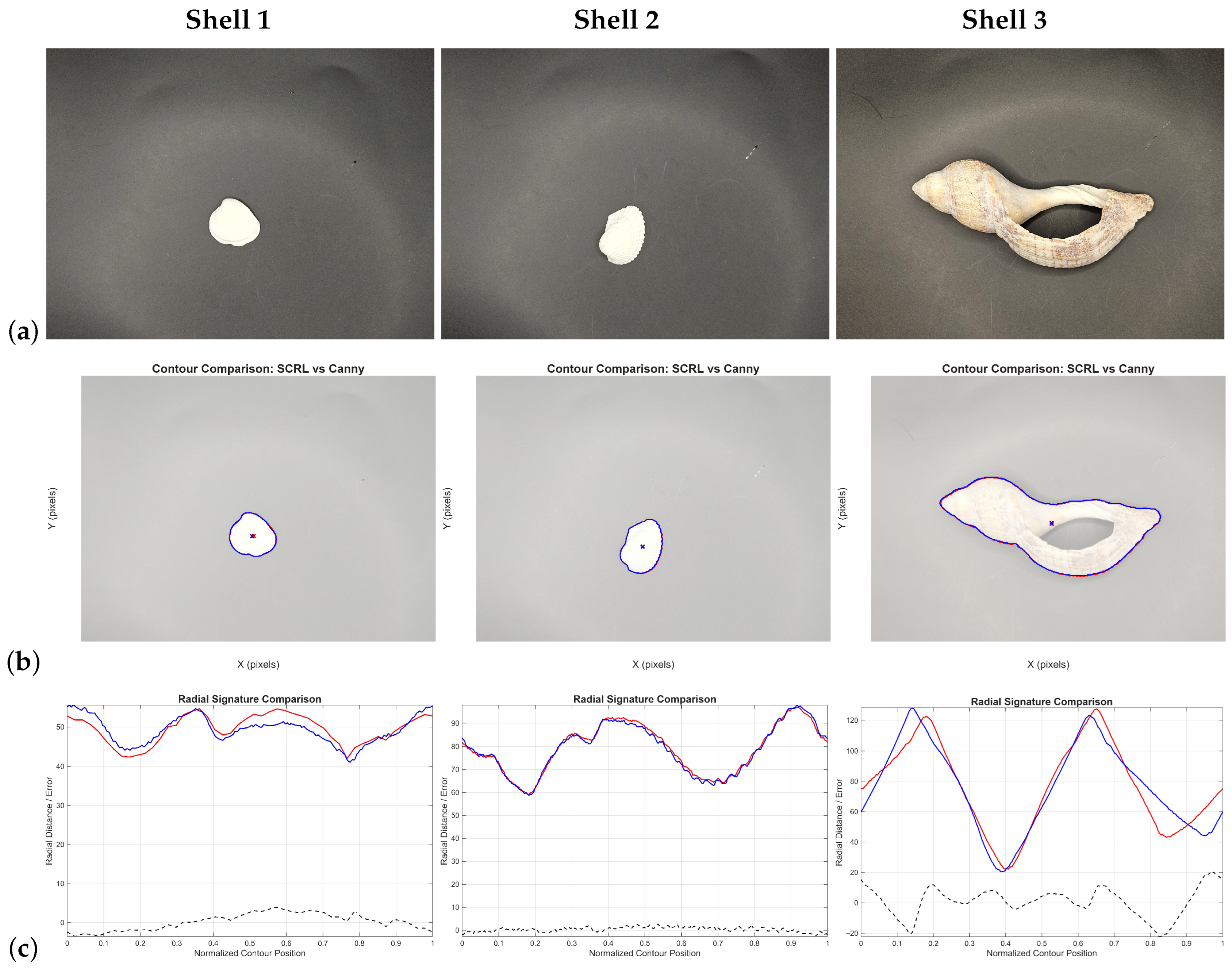
In the shell objects, LRCT is more stable in regions with smooth curvature but exhibits greater difficulty in areas with abrupt contour changes. This occurs because such discontinuities repeatedly fall within the analysis region, causing the algorithm to average their contributions and consequently propose a descriptive line. The radial signatures show small phase shifts and amplitude variations, yet they remain strongly correlated. In Shell 3, the maximum error of 21 px occurred in a relatively large specimen where a local misalignment arose during contour construction. Nonetheless, both results are considered correct.

Finally, based on the data in Table 1, the temporal cost per sample was estimated for both methods. On average, Canny+Moore requires approximately $0.10\mathrm{ms}$ per sample, while LRCT requires about $0.44\mathrm{ms}$, representing an increase of four- to five-fold in computational cost per point. This result is expected, as LRCT performs a region-based analysis rather than relying solely on local gradient information.

5. Discussion

Overall, the proposed procedure avoids the explicit construction of a closed binary contour image—as is typically performed after edge detection in the Canny algorithm—and instead proceeds directly to the organized and evenly spaced chaining of the points that represent the contour, starting from a previously computed edge map. In this way, it produces the contour representation that is traditionally obtained by combining Canny-based edge detection with Moore tracing.

The experimental results show that the method significantly reduces the number of points required to represent the contour, with decreases ranging from 43% to 84%, depending on the control parameters $d_b$ and T. This reduction is achieved without compromising either the geometric fidelity or the spatial distribution of the contour.

A notable property of the LRCT method is the greater stability observed both in the generated contours and in the corresponding radial signatures when compared to the Canny+Moore approach. While the latter depends on pixel chaining guided by gradient directions and on forcibly closing the contour—introducing stair-like artifacts unrelated to the original geometry—the proposed method yields samples whose existence is validated within the actual boundary. This results in a smoother and more faithful sequence of the contour. Such behavior suggests that the efficiency of representation can be particularly advantageous for objects with smooth morphologies or gradual transitions, such as natural materials or handcrafted artifacts.

However, this same characteristic may cause very small-scale discontinuities to be smoothed out or not recorded when their size is smaller than the exploration region, as observed in the case of shell 2 in Figure 21.

Furthermore, strong geometric coherence is maintained because the sampling relies on the spatial selection of points in the $XY$ plane. This is an advantage over uniform sampling schemes based solely on position within a discrete chain, since spatial selection adapts to the local geometry of the contour rather than depending on fixed intervals that may be insensitive to structural variations.

Regarding execution time, the LRCT method did not outperform the Canny+Moore combination, since it requires evaluating each point within a search region larger than the immediate pixel neighborhood. Although this increases computational cost, it also ensures a more robust and reliable tracking of the contour trajectory.

Finally, it is important to recall that classical computer vision methods are sensitive to the quality of the input image and to the conditions under which it is acquired. Unfavorable illumination—such as excessive brightness, pronounced shadows, or low contrast—can hinder contour characterization with LRCT. In our experiments, such conditions produced local deviations toward inner or outer areas influenced by secondary contours or surrounding elements (see arrowhead 1 in Figure 18). This behavior is consistent with the inherent limitations of traditional image-processing pipelines.

Furthermore, the present work does not position LRCT as a replacement for modern contour-extraction frameworks based on convolutional neural networks, but rather as a lightweight and transparent alternative for scenarios with controlled acquisition conditions, limited or unavailable training datasets, or restricted computational resources. A quantitative comparison against deep learning-based contour detectors remains an important direction for future research to contextualize the absolute performance of LRCT within the current state of the art.

6. Conclusions

The results confirm that the LRCT method adequately represents the contours of the analyzed objects. By directly generating the organized edge coordinates instead of relying on an intermediate image, the procedure aligns with a classical computer vision approach oriented toward geometric continuity rather than pixel-to-pixel connectivity. This characteristic facilitates the immediate application of discrete-signal analysis techniques—such as the independent evaluation of the X and Y components, radial signatures, cross-correlation, or the discrete Fourier transform—for purposes of representation, classification, or shape recognition.

The method also yields a significantly smaller number of samples without compromising boundary fidelity, owing to the spatially regular selection of representative points. This efficiency is particularly relevant in contexts where data reduction and stability across samples are essential for quantitative analysis.

However, the quality of the contour and the execution time depend on the size of the analysis region and on the search distance, parameters that must currently be defined manually by the user based on the object’s appearance and the image conditions. Although future developments may enable these values to be adjusted automatically according to the characteristics of the object and the size of the image, further studies will be required to establish optimal and reproducible relationships between these parameters.

While the computational cost per sample generated with LRCT can be approximately four times higher than that of the Canny+Moore approach, this increase is offset by the substantial reduction in the total number of samples, by the geometric fidelity obtained, and by the confirmation of the initial hypothesis: a more accurate contour reconstruction is achieved when the search is based on a spatial neighborhood larger than that of an isolated pixel.

Although the method requires specific conditions in both the photographic acquisition stage and the image processing stage, these requirements are consistent with standard documentation and treatment practices in archaeology and in automation processes within engineering. By integrating naturally into these workflows, the method constitutes an effective alternative to classical approaches, while also avoiding the training costs associated with deep learning-based methods.

Finally, the quality of the contours obtained positions LRCT as a suitable tool for the characterization and classification of archaeological materials. Its application can provide benefits in shape-related studies—where boundary geometry reflects manufacturing and preservation attributes—in analyses of association between fragments or related elements, and in the cataloging of large collections that require automated, consistent, and efficient solutions.