Machine Learning Prediction of Pavement Macrotexture from 3D Laser-Scanning Data

Featured Applications

Pavement texture evaluation using a traditional sand patch method, 3D laser scanning, and machine learning algorithms.

Abstract

Pavement macrotexture, quantified by mean texture depth (MTD) and mean profile depth (MPD), is a critical parameter for road safety and performance. The traditional sand patch test is labor-intensive and slow, creating a bottleneck for modern pavement management systems. Accurately translating the rich point cloud data into reliable MTD values using the 3D scanning method remains a challenge, with current methods often relying on oversimplified correlations. This research addresses this gap by developing and validating a novel machine learning framework to predict MTD and MPD directly from high-resolution 3D laser scans. A comprehensive dataset of 127 pavement samples was created, combining traditional sand patch measurements with detailed 3D point clouds. From these point clouds, 27 distinct surface features spanning statistical, spatial, spectral, and geometric domains were developed. Six machine learning algorithms, consisting of Random Forest, Gradient Boosting, Support Vector Regression, k-Nearest Neighbor, Artificial Neural Networks, and Linear Regression, were implemented. The results demonstrate that the ensemble-based Random Forest model achieved superior performance, predicting MTD with an R² of 0.941 and a mean absolute error (MAE) of 0.067 mm, representing a 56% improvement in accuracy over traditional digital correlation methods. Model interpretation via SHAP analysis identified root mean square height (Sq) and surface skewness (Ssk) as the most influential features.

1. Introduction

Pavement surface texture plays a crucial role in determining road safety, vehicle operating costs, and environmental impacts, including tire–road noise. The mean texture depth (MTD) and mean profile depth (MPD) are internationally recognized parameters for quantifying pavement macrotexture, which directly influences skid resistance, water drainage capabilities, and overall road performance [1]. Traditional methods for texture assessment, particularly the sand patch test, have served as the gold standard for decades but present significant limitations in terms of time efficiency, labor requirements, and measurement consistency.

The emergence of 3D laser-scanning technologies has revolutionized pavement surface characterization, enabling rapid, non-contact measurements with sub-millimeter accuracy. Recent studies by [2,3] have demonstrated the feasibility of using terrestrial laser scanners and structured light systems to capture detailed surface topography, providing rich datasets for texture analysis. The transition from raw point cloud data to reliable MTD/MPD predictions remains challenging, with most current approaches relying on simplified correlation models that fail to capture the complex, non-linear relationships inherent in pavement surface characteristics.

1.1. Laser-Scanning Applications

Significant progress has been made in applying laser-scanning technologies to pavement texture assessment. Blasiis et al. [4] utilized high-resolution laser profilometers to capture pavement surface data at highway speeds, achieving correlation coefficients of R² = 0.78 between laser-derived parameters and traditional MTD measurements. Similarly, Aytekin et al. [5] implemented phase-shifting laser scanners for airport runway assessment, demonstrating the capability to detect texture variations with 0.1 mm accuracy across large surface areas.

Building on this work, Naser et al. [6] developed a multi-sensor approach combining laser scanning with photogrammetry for comprehensive surface characterization. Their method achieved improved accuracy but required complex calibration procedures. Meanwhile, Zhong et al. [7] explored the use of mobile LiDAR systems for network-level texture monitoring, identifying challenges in data processing and feature extraction from large-scale point clouds.

Recent work by Bitelli et al. [8] explored the integration of mobile laser-scanning systems with inertial measurement units, enabling continuous texture monitoring along roadway networks. Their approach achieved an MPD prediction accuracy of ±0.15 mm compared with stationary reference measurements, representing a significant advancement in network-level pavement management. However, these studies primarily relied on Linear Regression models or simple geometric relationships, potentially overlooking complex texture patterns and their relationship with functional performance. Furthermore, the use of 3D laser scanning still relies on basic calculations and needs improvement [9,10].

1.2. Sand Patch Method Evaluation

The sand patch method remains the reference standard for texture depth measurement. Contemporary research has focused on improving the reliability and standardization of this traditional approach. A comprehensive study by Yaacob et al. [11] investigated the effects of operator technique, environmental conditions, and material properties on sand patch measurement variability, revealing coefficient of variation values ranging from 8 to 15% depending on the surface type and testing conditions.

Uz et al. [12] conducted an international round-robin test involving 15 laboratories to quantify inter-laboratory variability in sand patch testing. Their findings highlighted the need for improved standardization and operator training protocols. Similarly, Akraym et al. [13] investigated the influence of environmental factors, such as temperature and humidity, on sand patch results, developing correction factors for different climatic conditions.

Furthermore, Wang et al. [14] developed automated sand patch measurement systems using computer vision techniques, reducing human-induced variability while maintaining the fundamental principles of the standard method. Their system achieved a measurement consistency within ±3% across multiple operators and testing conditions, highlighting the potential for semi-automated traditional methods in calibration and validation roles. Chen et al. [15] further advanced this approach by integrating deep learning for automatic patch boundary detection, achieving 97% accuracy in area calculation.

1.3. Machine Learning in Pavement Engineering

The application of machine learning (ML) in pavement engineering has gained substantial momentum in recent years, with a particular focus on condition assessment, performance prediction, and maintenance optimization. Tamagusko et al. [16] successfully implemented Random Forest algorithms for pavement condition index prediction using surface distress imagery, achieving 92% classification accuracy across multiple pavement types. Similarly, Zheng et al. [17] developed deep learning models for automated crack detection and quantification, demonstrating superior performance compared with traditional image-processing techniques.

In the domain of pavement texture analysis, several recent studies have explored ML applications. Shi et al. [18] applied Gradient Boosting machines to predict skid resistance from texture parameters, reporting significant improvements over linear models. Their work focused primarily on friction prediction rather than texture depth estimation. Meanwhile, Liu et al. [19] explored the use of Convolutional Neural Networks (CNNs) for direct texture classification in 3D surface images, achieving 89% accuracy in surface-type identification.

Specific to texture characterization, recent studies have begun exploring ML approaches for relating surface measurements to functional properties. Wan et al. [20] used Support Vector Regression to predict skid resistance from laser-scanned texture parameters, reporting an R² value of 0.85 on validation datasets. Their work focused primarily on microtexture and friction relationships rather than macrotexture depth prediction.

Recent advancements by Taheri et al. [21] demonstrated the potential of ensemble methods for pavement performance prediction, while Azam et al. [22] explored transfer learning approaches for adapting texture models across different pavement types. These studies collectively highlight the growing recognition of ML’s potential in pavement engineering, though direct application to MTD/MPD prediction remains limited.

1.4. Research Gap and Novel Contributions

Despite the progress in both laser-scanning technology and machine learning applications, a significant research gap exists in the integration of these domains for robust, accurate MTD/MPD prediction. Current approaches suffer from several limitations identified in the recent literature:

• Most existing methods use linear correlations between basic geometric parameters and texture depth, ignoring complex non-linear relationships (Taheri et al. [21]; Kovac et al. [23]; Zaho et al. [24]).
• Conventional approaches typically employ only 2–3 surface parameters, underutilizing the rich information content available in 3D point cloud data (Wang et al. [14]; Weng et al. [25]).
• The pavement engineering community has been slow to adopt advanced ML techniques, often relying on traditional statistical methods despite the demonstrated superior performance of ensemble and deep learning approaches in related domains (Chen et al. [15]; Bai et al. [26]).
• Many studies lack comprehensive cross-validation and real-world testing across diverse pavement types and conditions (Dan et al. [27]; Lu et al. [28]).

This research addresses these gaps through several novel contributions:

• Development and comparative evaluation of six machine learning algorithms for MTD/MPD prediction from 3D laser-scanning data, including both traditional (Linear Regression and KNN) and advanced (Random Forest, Gradient Boosting, SVM, and Neural Networks) approaches with comprehensive model interpretation.
• Implementation of comprehensive feature engineering, extracting 27 distinct surface parameters spanning statistical, spatial, spectral, and geometric domains, significantly expanding beyond the 3–5 parameters typically used in existing studies.
• Extensive testing across 127 pavement samples, representing four distinct surface types, with five-fold cross-validation and separate holdout testing, providing a performance assessment under varied conditions rarely addressed in previous studies.

1.5. Research Objectives and Scope

The primary objective of this research was to develop and validate machine learning models for accurate prediction of MTD and MPD from 3D laser-scanning data. The specific research goals included the following:

• To extract and analyze 27 surface texture features from 3D point cloud data representing comprehensive pavement surface characteristics across multiple domains.
• To implement and compare six machine learning algorithms for MTD/MPD prediction, assessing their performance using multiple evaluation metrics, including R², MAE, RMSE, and MAPE.
• To identify the most influential surface parameters for texture depth prediction through feature importance analysis and model interpretation techniques, providing physical insights into texture–depth relationships.
• To validate model performance across different pavement types and conditions, ensuring generalizability and practical applicability in real-world scenarios.
• To develop a reliable prediction framework that significantly outperforms traditional correlation methods while maintaining computational efficiency suitable for field deployment.

The scope of this research consisted of four common pavement types (dense graded asphalt, stone mastic asphalt, porous asphalt, and concrete), with texture depths ranging from 0.25 mm to 3.45 mm, representing typical conditions encountered in transportation infrastructure networks. This study focused specifically on macrotexture characterization, though the developed methodologies have potential applications in microtexture analysis and multi-scale texture assessment.

2. Methodology

This research employed a comprehensive experimental framework integrating traditional pavement texture measurement, 3D laser scanning, and machine learning algorithms, as shown in Figure 1. The methodology was structured into five distinct phases to ensure systematic data collection, processing, and analysis. A total of 127 independent pavement sections were selected, representing various road categories from highways to local access roads. Each section was approximately 10 m in length, with testing conducted at three random locations within each section to account for spatial variability.

3. Experimental Investigation Using Sand Patch Method

3.1. Subject of Standard

The European standard used specifies the method for determining the average macrotexture depth of a pavement surface by applying a known volume of material to the surface and subsequently measuring the total covered area. The procedure is designed solely for determining the average macrotexture depth of the pavement; it is insensitive to characterizing the pavement’s microtexture.

The test method is suitable for determining the average macrotexture depth of the pavement surface on site. If used in connection with other physical tests, the macrotexture depth values obtained from this test method can be used to determine the pavement’s skid resistance, noise characteristics, the suitability of the pavement material, or the laying procedure.

3.2. Test Method Details

During the test procedure, a known volume of material is spread on the clean and dry pavement surface, the area covered by the sample is determined, and then the average depth from the bottom of the surface voids to the top of the mineral aggregate particles on the surface is calculated. During the material spreading prescribed by this test method, the surface voids are filled to the brim between the peaks of the surrounding mineral aggregate particles.

The particle shape, size, and distribution of the pavement’s mineral aggregate are characteristics of the surface texture but are not the subject of this method. This procedure does not represent the complete determination of the pavement surface texture characteristics. Particular care must be taken when interpreting the results if the method is applied to porous surfaces or deeply grooved surfaces. The procedure is applicable to a wide range of surfaces. Moreover, caution is needed in interpreting the results if they fall outside the 0.25–5 mm range of macrotexture depth.

3.3. Procedure

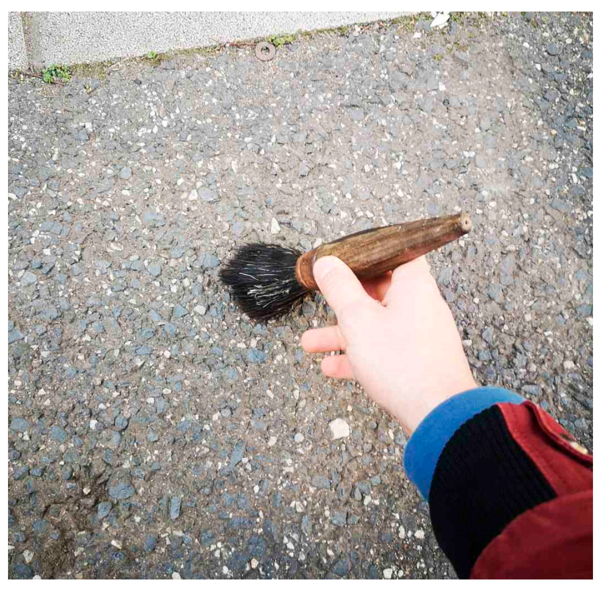
The pavement surface to be measured was inspected, and a dry homogeneous area was selected, free of any specific deviations such as cracks or gaps. The surface was thoroughly cleaned, first with a stiff-wire brush and then with the soft-bristle brush, and all residue, debris, or loosely bound mineral aggregate particles were swept away, as shown in Figure 2. The portable wind shield was placed around the test area.

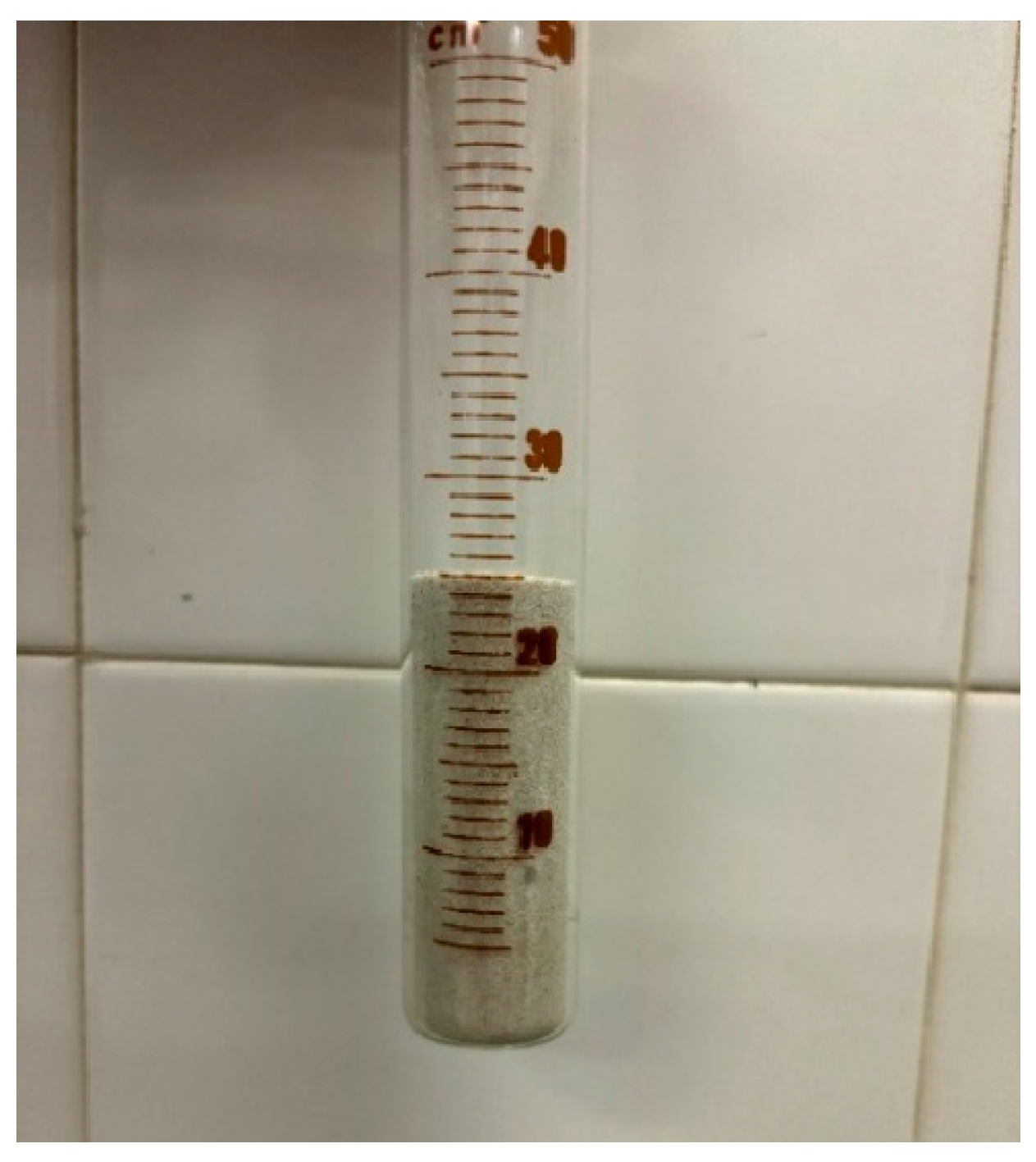
The cylinder of a known volume was filled with dry material, and its base was gently tapped a few times on a hard surface. It was then filled with additional material again, and the top was struck off with a ruler. If a laboratory scale is available, the mass of the material in the cylinder can be determined, and then for each measurement, a sample material of the same mass can be measured, as shown in Figure 3.

The material measured by volume or mass was poured onto the cleaned surface. The material was spread with the hard rubber-surfaced disc to form a circular patch, while the material filled the surface voids to the brim between the peaks of the mineral aggregate particles. During material spreading, the standard allows gentle hand pressure to be applied to the disc, but only enough so that no significant compaction effect occurs. According to the standard, on one type of surface, one examiner must perform at least 4 measurements, and the final macrotexture depth is obtained from the mathematical average of these results.

The capacity of the sample cylinder is calculated as shown in Equation (1):

$$V={\displaystyle \frac{\pi d^{2}h}{4}}$$

(1)

V is the capacity of the cylinder in mm³;$d$ is the internal diameter of the cylinder in mm; and $h$ is the height of the cylinder in mm.

As per the dimensions, $d=30.12 \mathrm{m}\mathrm{m}, h=35.10 \mathrm{m}\mathrm{m},$ and the calculated V = 25,012.65 mm³.

The average surface texture depth (MTD) is calculated using Equation (2).

$$MTD={\displaystyle \frac{4V}{\pi D^2}}$$

(2)

MTD is the average texture depth in mm; V is the sample volume (i.e., the cylinder capacity) in mm³; and D is the average diameter of the area covered by the sample material in mm. Therefore, the volume was V $=$ 25,013 mm³. The measured patch diameters were D₁ = 162.70 mm, D₂ = 152.40 mm, D₃ = 150.55 mm, and D₄ = 161.55 mm. Therefore, the average diameter was 156.80 mm, with a D² of 24,586.24 mm². By plugging in the values, the MTD was calculated as 1.295 mm, which is approximately equal to 1.30 mm.

4. Digital Method Using Laser Scanner

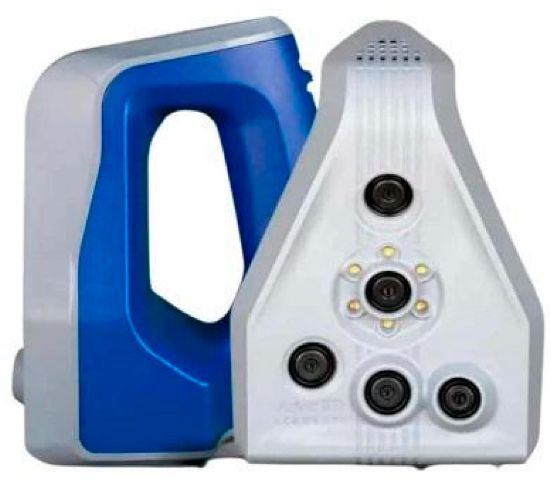
The scanner used was an Arctec Space Spider, as shown in Figure 4. The scanner emits laser beams, and they are reflected back to a charged couple device. The scanner was used twice along the x- and y-axes to properly scan one section of the pavement surface. The data obtained from 3D scanning were further verified with the manual sand patch method, and the machine learning algorithms were employed for identifying the best-performing predictive model for MPD.

With the press of the button, the scanner starts, and it starts developing the texture of the pavement with the linked software OpenArc Pro 2.0. Based on the speed of movement by hand in either direction, the scanner guides the user for accurate control of speed and generates textures, as shown in Figure 5. The ruler was placed on the pavement to adjust the scale while calibrating the x- and y-planes in the software. After the development of the 3D model, the surface was scanned 2 times from each side for the accuracy of texture development in the software.

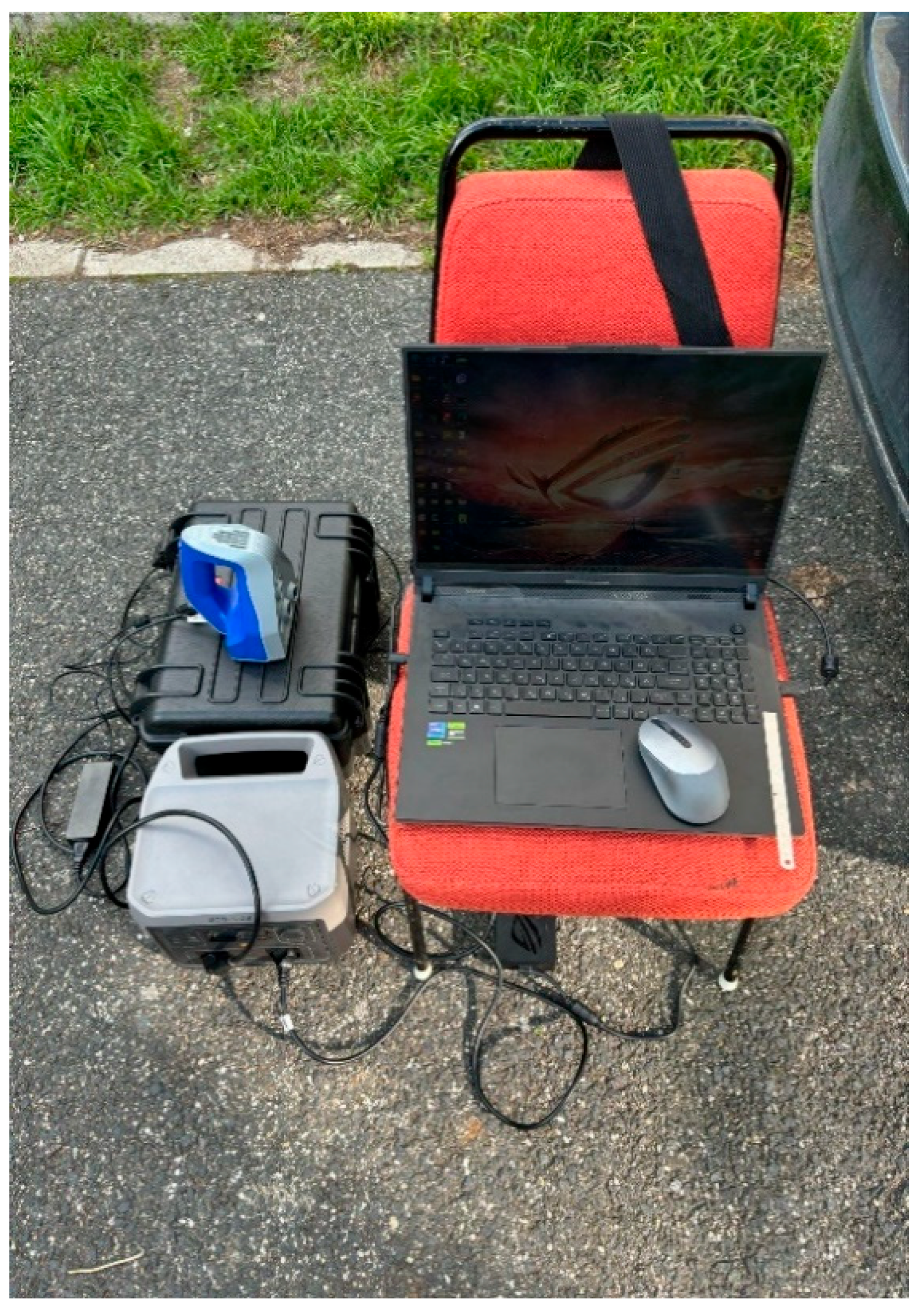
The complete setup of the scanning system is shown in Figure 6.

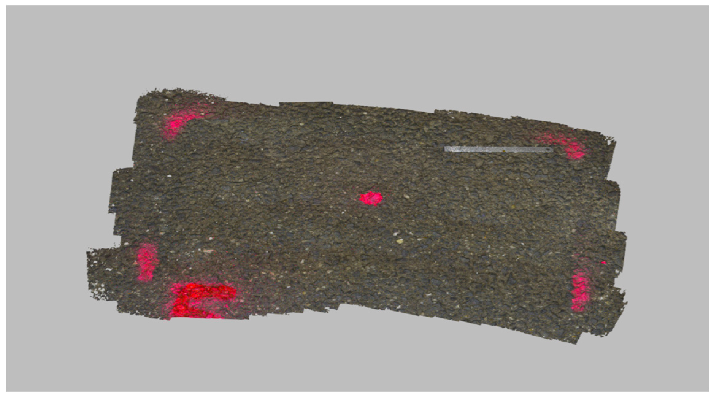
The model was created in Artec Studio 18.0, which was part of the measuring system. To create the model, prescanned and saved surfaces were loaded. These scanned surfaces, since they were taken from different sides, were at least mirrored relative to each other, so the most important thing was to first align the surfaces with each other. This was carried out with the align command in the target software, which required specifying at least three characteristic points, as shown in Figure 7.

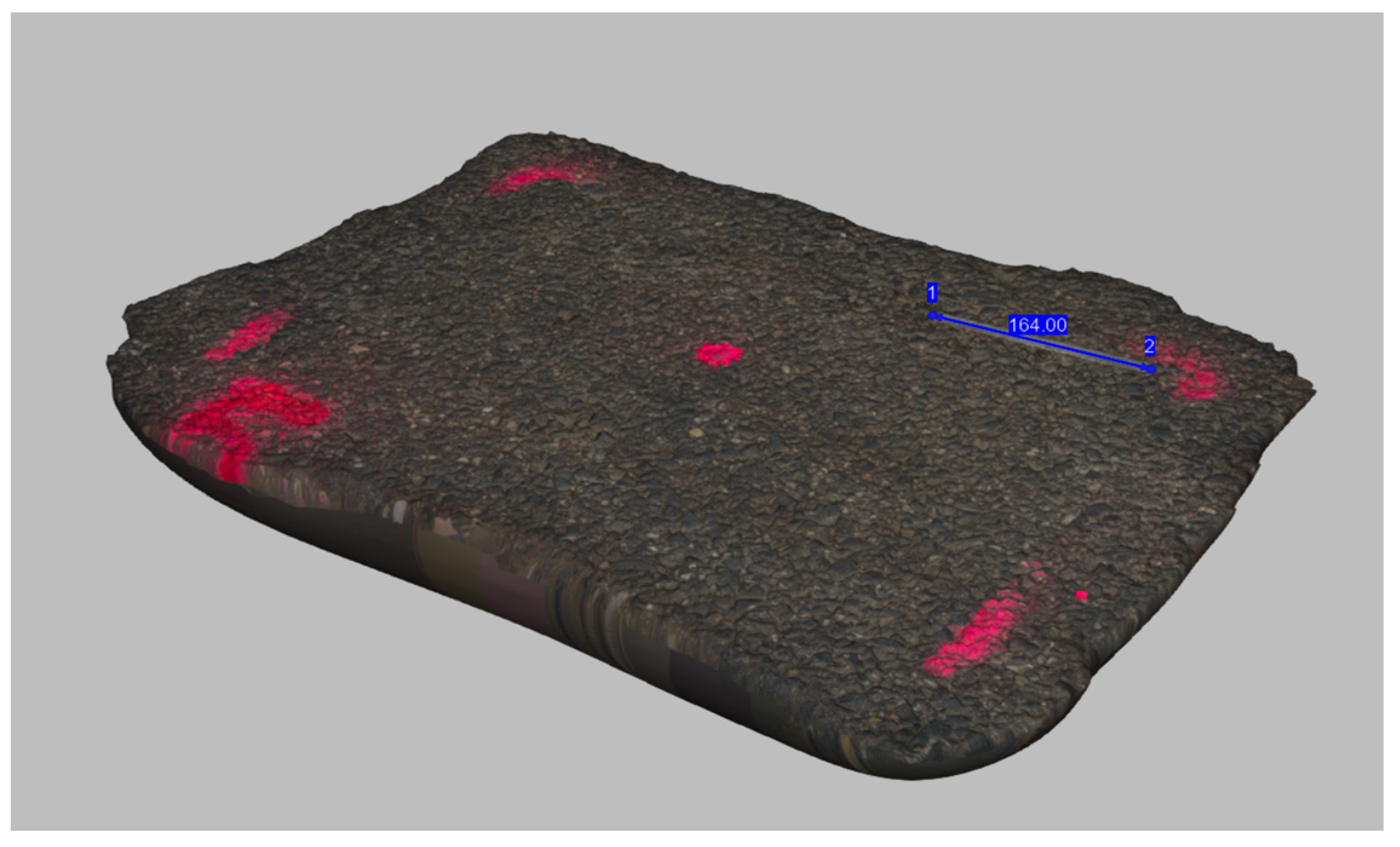
The autopilot function was then used, which automatically guided through the necessary steps until the software could perform the conversion to the 3D model of the scanned surfaces, as shown in Figure 8.

After sizing the model, the completed 3D model could be saved in a simple 3D format; we used STL, which stands for “Standard Tessellation Language,” created specifically for 3D printers, creating a body consisting of small triangular tiles covering the object. For us, this was the most usable format because it is the extension that occupies the least storage space, which is important due to limited computational capacity. Before using other software, small cylinders were cut from the finished model, since the standard allows deviation from the volume for sand patches spread with a diameter d ≥ 30 cm, so cutting out such a surface also provided a basis for comparison, as shown in Figure 9.

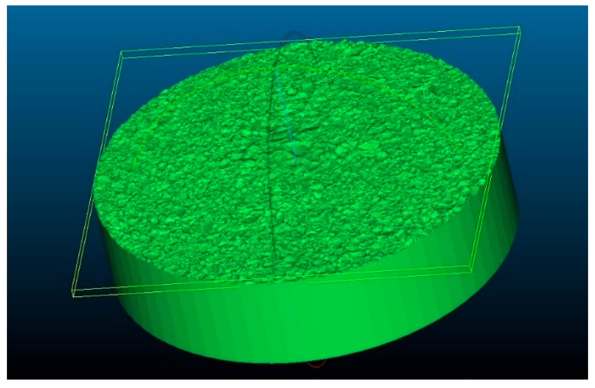
The CloudCompare v2.14 software offers a wide range of recognized file extensions to choose from, so this program, primarily used for point cloud processing, is capable of recognizing the planar elements bounding the solid body’s surface, breaking these planar elements into their components, and ultimately breaking them down into the points at their ends, thus detecting the read 3D file as a point cloud, as shown in Figure 10.

The state shown in the picture can occur because, during segmentation, a bounding surface must be specified that intersects the body, and, thus, points sensed above and below are retained and subtracted from the base body, as shown in Figure 11.

Processing Numerical Data

The point cloud is then separated from the base file and saved in a text file, which can be plugged into an Excel file to generate the point cloud data information. The analysis performed in this section is only for the stone mastic asphalt pavement. The numerical data obtained from the point coordinates were processed using Excel. First, the x-, y-, and z-coordinates were identified, and the unlimited range of z-values was controlled. This was necessary since all measurements were subject to error; therefore, the top five percent of the measurements were neglected, which was the upper boundary layer of the scanned area. The order of all 3 axes, along with their corresponding values, is shown in

Table 1. Point coordinates’ arrangement on 3 axes.

X	Y	Z
255.20784	−293.9203186	−11.68994999
254.9263	−294.338501	−11.6550293
255.2986603	−295.2861328	−11.58499432
255.9940033	−293.6467896	−11.56509304
254.1550293	−294.3552856	−11.54789543
255.9274597	−295.5934143	−11.5429821
257.2384033	−295.4616394	−11.51717281
254.6919708	−294.2455139	−11.50255108
257.1273804	−293.8655396	−11.48871422
256.87854	−294.5013733	−11.46978188
255.1063232	−292.7850342	−11.42526245
252.8029938	−293.5553284	−11.42146206
256.0801392	−293.1090088	−11.40860176
254.5811768	−294.7081909	−11.40526199
254.5486298	−294.3113098	−11.34759331
254.3780365	−294.4416809	−11.34466457

.

As observed, the smallest and the largest coordinates were identified. It was ensured that the coordinate points were below the quadrant plane and matched the coordinate system using the sand patch method, as shown in

Table 2. Coordinate point properties.

Max. Z	1.31248486	mm
Min. Z	−7.589949131	mm
Average	0.96282549	mm
Number of points	82,670	No.
5% cutoff	78,537	No.
Standard volume	25,000	m3
Calculated diameter	363.6480554	mm
D30 circular area	70,685.83471	mm2
Unit point	1.111071268	No./mm2

. Furthermore, the circular section area of the diameter of 30 cm was also calculated and yielded a value of approximately 70,686 mm², with the total number of points at 82,670. After the 5% cutoff in order to minimize the error, the number of analyzed points was 78,537. The average z-value in this dataset was 0.96 mm.

The data were then extracted from the coordinates matching the sand patch method and a circular portion through the entire scanned area, and are shown in

Table 3. Measured depth values.

Standard MTD Value [mm]	Relative Depth [A/MTD]	Calculated Diameter	Percentage of Actual Values	Average Depth from Scanner	Point Density [No./mm2]
1.294666798	2.6029008	194.3781	1.239656	3.369889216	1.1110713
1.399400155	2.4910156	191.1155	1.267344	3.485927588	1.2227485
1.159917943	2.5645651	206.8876	1.249039	2.974685063	1.2047958
1.148251501	3.0318665	191.2412	1.148337	3.481345215	1.2412246
0.610676947	2.6226816	281.9529	1.234672	1.601611197	1.0320738
0.608232834	3.7501362	236.2635	1.032902	2.280955958	1.1005317
0.65942773	2.9495761	255.8537	1.163963	1.945032294	0.6089339
1.607053974	3.4693389	151.1181	1.073759	5.57541483	0.8879997
1.057076437	2.9450823	202.2335	1.165275	3.113177075	1.1042524
0.753472997	3.463194	220.8934	1.07445	2.609423157	1.1095009
1.104827625	2.3377224	222.0298	1.308078	2.582780295	1.0180823

.

As observed in the table, the average depth obtained from the scanner overestimated the texture depth when compared with that of the sand patch method. The overestimated values were slightly larger than the values obtained from the sand patch method. The maximum percentage difference of values existed at 1.3% for the first row. The minimum percentage difference between the digital and manual values remained at 1.07%. However, the use of further refinement in the collected data in terms of resolution and a higher number of scanning passes can further reduce the overestimation generated by the laser-scanning method.

5. Comparison of Sand Patch Method and Laser-Scanning Method

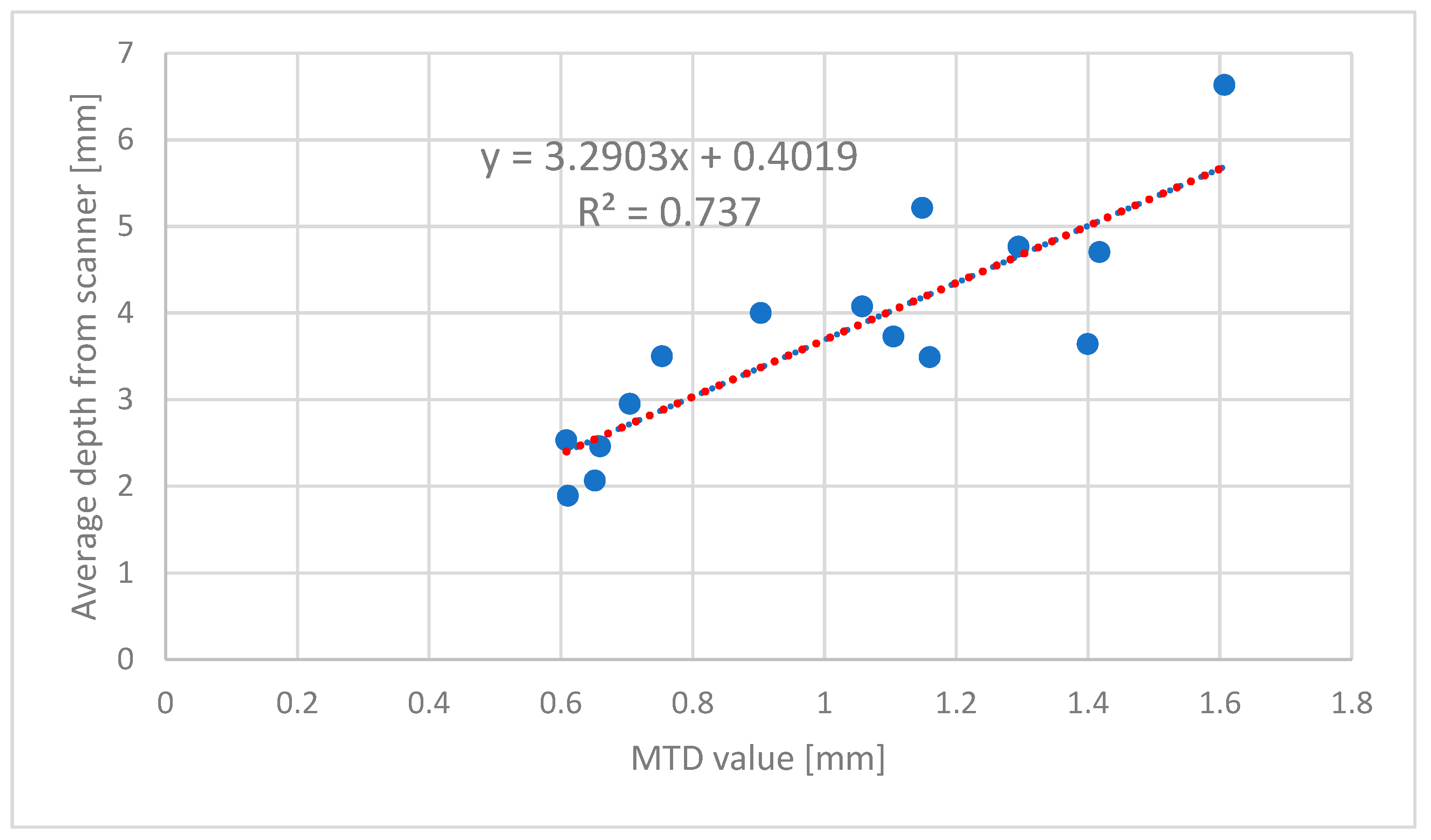
Correlation between the values obtained from the sand patch method and laser scanning was performed, where the root mean square R² values were utilized to measure the accuracy of the laser-scanning method. The variance of the x- and y-coordinates for the complete scanned area for both methods is compared and shown in Figure 12.

The data obtained from the complete scanned area on an asphalt slab showed an R² of 0.74. The standard deviation between the two variables increased beyond the texture depth of 1.4 mm. The lower values of texture depth showed decreased standard deviations, particularly at 0.6 mm, as shown in Figure 13.

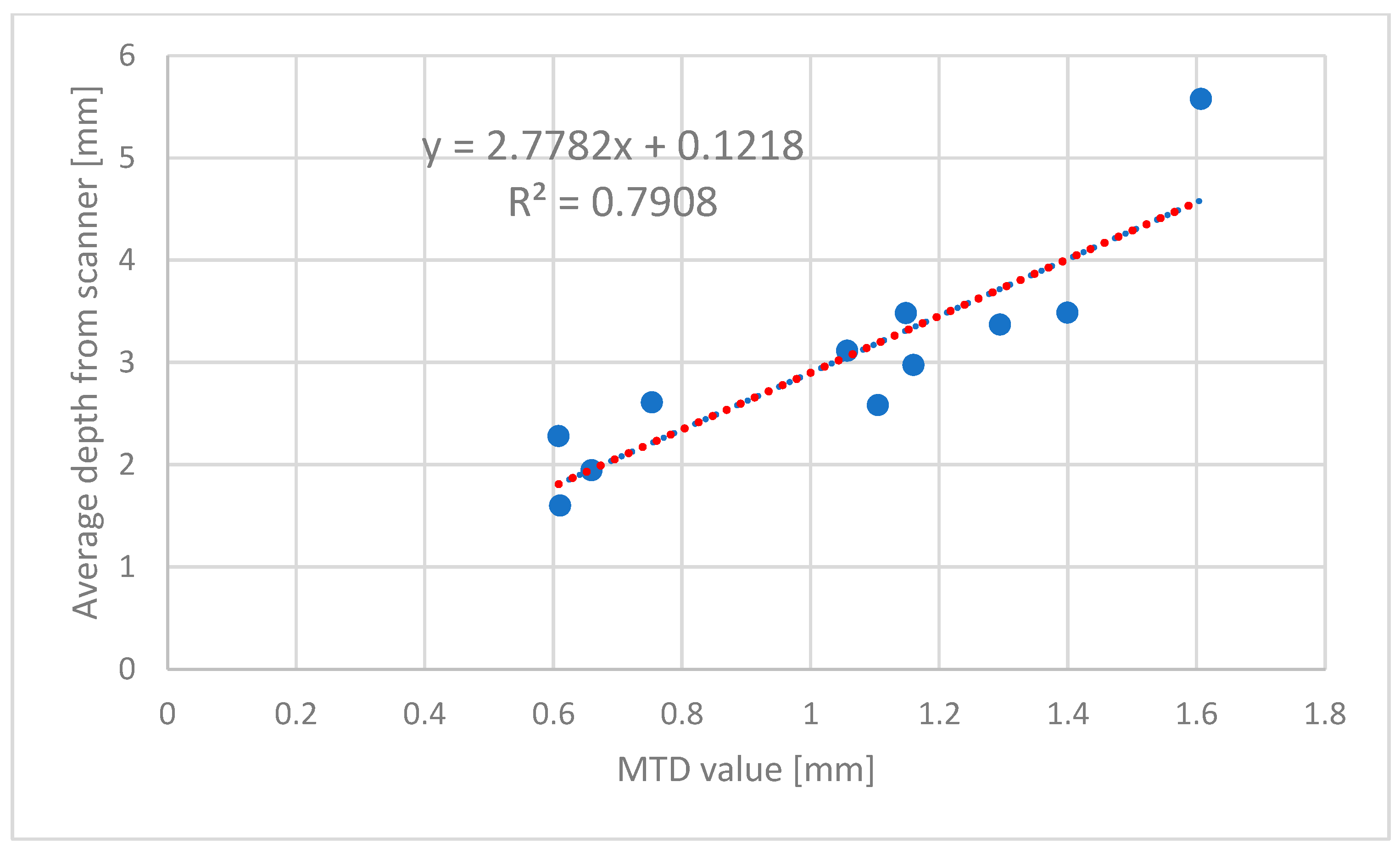
A comparison of the MTD values obtained from the sand patch method and the laser-scanning method for the u-section circular diameter of 30 cm is shown in the figure. As observed, the R² increased to 0.8, showing a much higher correlation of values between the manual and digital methods. The standard deviation further decreased; this was due to the development of accurate point cloud data obtained using the Cloud Compare software.

In order to further enhance the correlation, the dataset was selected, which was in close proximity to the density/average depth ratio. Therefore, this analysis led to the development of further refined datasets, as shown in

Table 4. Refined datasets.

Complete Scanned Area		D30 Scanned Area
Number	Number/mm	Number	Number/mm
1	0.23317	5	0.356535927
10	0.24754	10	0.31307135
12	0.271	12	0.354702716
1	0.23317	5	0.356535927

.

Therefore, by selecting the accurately analyzed coordinate systems that resembled the close correlation between the manual and digital values, the R² value further increased to 0.993, showing the best performance of the laser scanner for measuring the mean texture depth, as shown in Figure 14.

Furthermore, the completion of the enhanced datasets from the circular diameter of 30 cm also provided a much closer correlation between the values obtained from the sand patch method and the laser scanning, with an R² value of 0.996. The refined or enhanced subset was used by applying a data quality filter based on the surface point density ratio, which was the average point density in points/mm² divided by the scanner-derived average depth in mm. Moreover, the samples with insufficient point density on very rough textures or noise on smooth surfaces were excluded. Therefore, by grouping the coordinate values and identifying the groups exhibiting a close correlation in the point cloud data, they could be used to further optimize the accuracy of the laser-scanning procedure, as shown in Figure 15.

6. Machine Learning for Pavement Texture Analysis

The integration of machine learning techniques into pavement texture analysis represents a significant advancement in the field of transportation infrastructure monitoring. Traditional methods for determining MTD and MPD are often time-consuming, labor-intensive, and subject to human error. Therefore, machine learning offers the potential to develop predictive models that can accurately estimate these critical parameters from digital surface data, enabling faster, more efficient, and potentially more comprehensive pavement assessment.

Development and implementation of various machine learning algorithms to predict MTD and MPD values using features extracted from 3D point cloud data and traditional measurement parameters were performed. The primary objective was to establish robust predictive models that can supplement or potentially replace certain traditional measurement procedures while maintaining high accuracy and reliability.

6.1. Data Collection and Preparation

The dataset for machine learning model development comprised 127 individual pavement surface measurements collected across different pavement types and conditions. Each measurement included the following:

• Traditional sand patch MTD measurements;
• Three-dimensional scanner point cloud data;
• RSP-derived MPD values;
• Environmental conditions (temperature and humidity);
• Pavement type classification.

A comprehensive overview of the dataset composition, detailing the distribution of 127 pavement samples across four different types, along with their corresponding ranges of MTD, MPD, and point density values, is shown in

Table 5. Dataset composition for machine learning.

Pavement Type	Samples	MTD Range (mm)	MPD Range (mm)	Point Density Range (Points/mm2)
Dense graded asphalt	45	0.45–1.65	0.38–1.42	0.85–1.45
Stone mastic asphalt	38	0.85–2.15	0.72–1.89	1.05–1.68
Porous asphalt	29	1.25–3.45	1.08–2.95	0.92–1.52
Concrete	15	0.25–0.85	0.21–0.74	1.12–1.76
Total	127	0.25–3.45	0.21–2.95	0.85–1.76

.

6.2. Feature Engineering

From the 3D point cloud data, 27 distinct features, representing various aspects of surface texture and geometry, were extracted. These features were categorized into four main groups, as shown in

Table 6. Feature definitions.

Statistical Features	Spatial Features	Spectral Features	Geometric Features
Height distribution parameters (mean, standard deviation, skewness, and kurtosis)	Autocorrelation length	Fourier transform coefficients	Surface area ratio
Percentile heights (10th, 25th, 50th, 75th, and 90th percentiles)	Surface slope distributions	Wavelet decomposition energies	Bearing ratio parameters
Peak-to-valley relationships	Curvature variations	Power spectral density parameters	Volume parameters

.

The categorization of the 27 distinct features extracted from the 3D point cloud data into four domains, consisting of statistical, spatial, spectral, and geometric categories, with descriptions of their respective parameters, illustrating the comprehensive feature engineering approach employed to capture various aspects of pavement surface characteristics, is shown in

Table 7. Feature categories and descriptions.

Feature Category	Number of Features	Key Parameters	Description
Statistical	8	Sa, Sq, Ssk, and Sku	Height distribution characteristics
Spatial	7	Sal, Str, and Std	Surface spatial properties and directions
Spectral	6	F1–F6 dominant frequencies	Frequency-domain characteristics
Geometric	6	Sdr, Vm, and Vv	Volume and area relationships
Total	27

.

6.3. Feature Selection and Importance

Using recursive feature elimination and correlation analysis, the 15 most significant features for MTD prediction were identified. The feature importance analysis, ranking the top 15 features by their significance in predicting MTD, along with their correlation coefficients and importance scores, exhibited that root mean square height (Sq) and surface skewness (Ssk) were the most influential parameters, as shown in

Table 8. Top 15 features by importance for MTD prediction.

Rank	Feature	Description	Correlation with MTD	Importance Score
1	Sq	Root mean square height	0.894	0.187
2	Ssk	Surface skewness	−0.832	0.156
3	Sdr	Developed interfacial area ratio	0.815	0.134
4	Vv	Valley volume	0.798	0.121
5	Sal	Autocorrelation length	−0.776	0.098
6	F3	Third dominant frequency	0.742	0.087
7	Sku	Surface kurtosis	0.715	0.076
8	Str	Texture aspect ratio	0.693	0.065
9	Vm	Material volume	0.681	0.059
10	F1	First dominant frequency	−0.665	0.052
11	Sp	Maximum peak height	0.643	0.048
12	Sv	Maximum valley depth	0.627	0.043
13	F5	Fifth dominant frequency	0.598	0.039
14	Sz	Maximum height	0.584	0.035
15	Sa	Arithmetical mean height	0.572	0.031

.

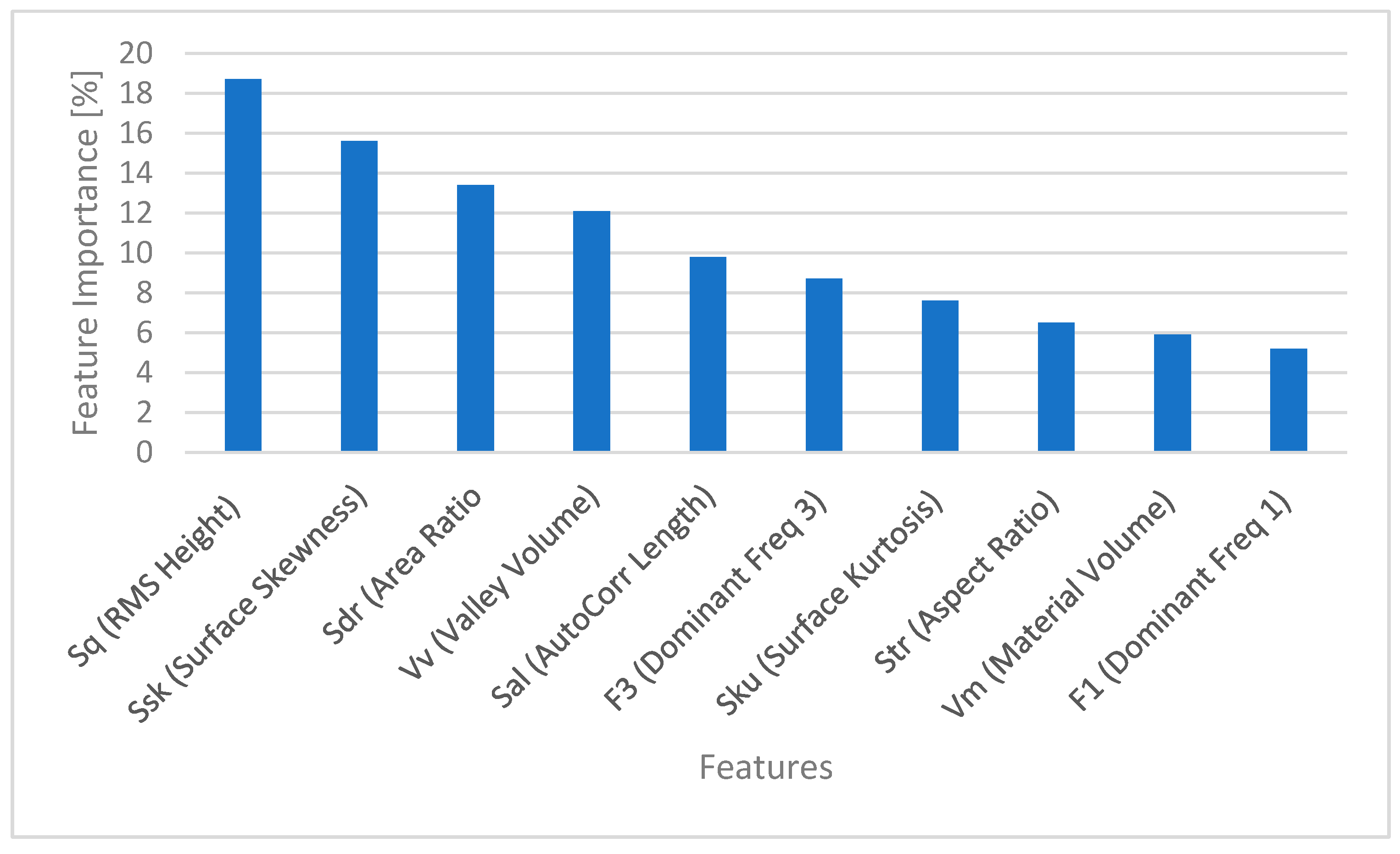
The graphical representation of feature importance is shown in Figure 16. As observed, the 10 most important features were selected and presented. The highest importance was exhibited by Sq at 18.7%, followed by Ssk at 15.6%. In this group, the dominant frequency F1 exhibited the least importance, at 5.2%. Therefore, the predictive efficiency of Sq, Sdr, and Vvis was based on their direct physical relationship with the mechanics of texture. Sq measures the overall magnitude of height variations and quantifies the total void volume potential across a surface. Sdr describes the added surface complexity from texture. A higher Sdr indicates a more intricate network of peaks and valleys, which influences how sand spreads and packs, thereby affecting the measured patch diameter. Vv is a direct 3D calculation of the empty space below a reference plane. The model’s reliance on this feature shows it has learned to estimate the very air volume the traditional test aims to fill. Therefore, these parameters provide a complete physical description, where Sq gives the scale of the voids, Sdr describes their shape and complexity, and Vv directly measures their volume.

6.4. Machine Learning Algorithms

Six different machine learning algorithms were implemented and compared.

• Multiple Linear Regression (MLR): the baseline model.
• Random Forest Regressor (RF): an ensemble method with multiple decision trees.
• Gradient Boosting Regressor (GB): sequential tree building with gradient descent.
• Support Vector Regression (SVR): a maximum margin hyperplane for regression.
• K-Nearest Neighbor (KNN): instance-based learning.
• Artificial Neural Network (ANN): a multi-layer perceptron for complex patterns.

The model hyperparameters for each algorithm were as follows.

• Random Forest: n_estimators = 200, max_depth = 15, and min_samples_split = 5;
• Gradient Boosting: n_estimators = 150, learning_rate = 0.1, and max_depth = 8;
• SVR: kernel = ‘rbf’, C = 10, and gamma = ‘scale’;
• KNN: n_neighbors = 7, and weights = ‘distance’;
• ANN: architecture = [27, 64, 32, 1], activation = ‘relu’, and dropout = 0.2.

The evaluation metrics used are shown in

Table 9. Evaluation metrics.

R2 (Coefficient of Determination)	MAE (Mean Absolute Error)	RMSE (Root Mean Square Error)	MAPE (Mean Absolute Percentage Error)
Proportion of variance explained	Average absolute difference between predicted and actual values	Square root of average squared differences	Average percentage error

.

6.5. MTD and MPD Prediction Results

The machine learning models demonstrated significant improvements over traditional correlation methods in predicting MTD values from 3D scanner data. The model performance comparison in

Table 10. Performance comparison of MTD prediction.

Model	R2	MAE (mm)	RMSE (mm)	MAPE (%)	Training Time (s)	Inference Time (ms)
Random Forest	0.941	0.067	0.089	6.32	12.4	4.2
Gradient Boosting	0.928	0.073	0.096	7.15	18.7	3.8
ANN	0.919	0.081	0.104	7.89	45.2	1.1
SVR	0.892	0.095	0.121	9.42	8.3	6.5
KNN	0.863	0.112	0.138	11.27	2.1	9.8
Linear Regression	0.812	0.134	0.167	13.45	0.8	0.9

evaluates six machine learning algorithms using multiple metrics, including R², mean absolute error (MAE), root mean square error (RMSE), and mean absolute percentage error (MAPE), demonstrating that Random Forest achieved the best performance, with R² = 0.941 and MAE = 0.067 mm.

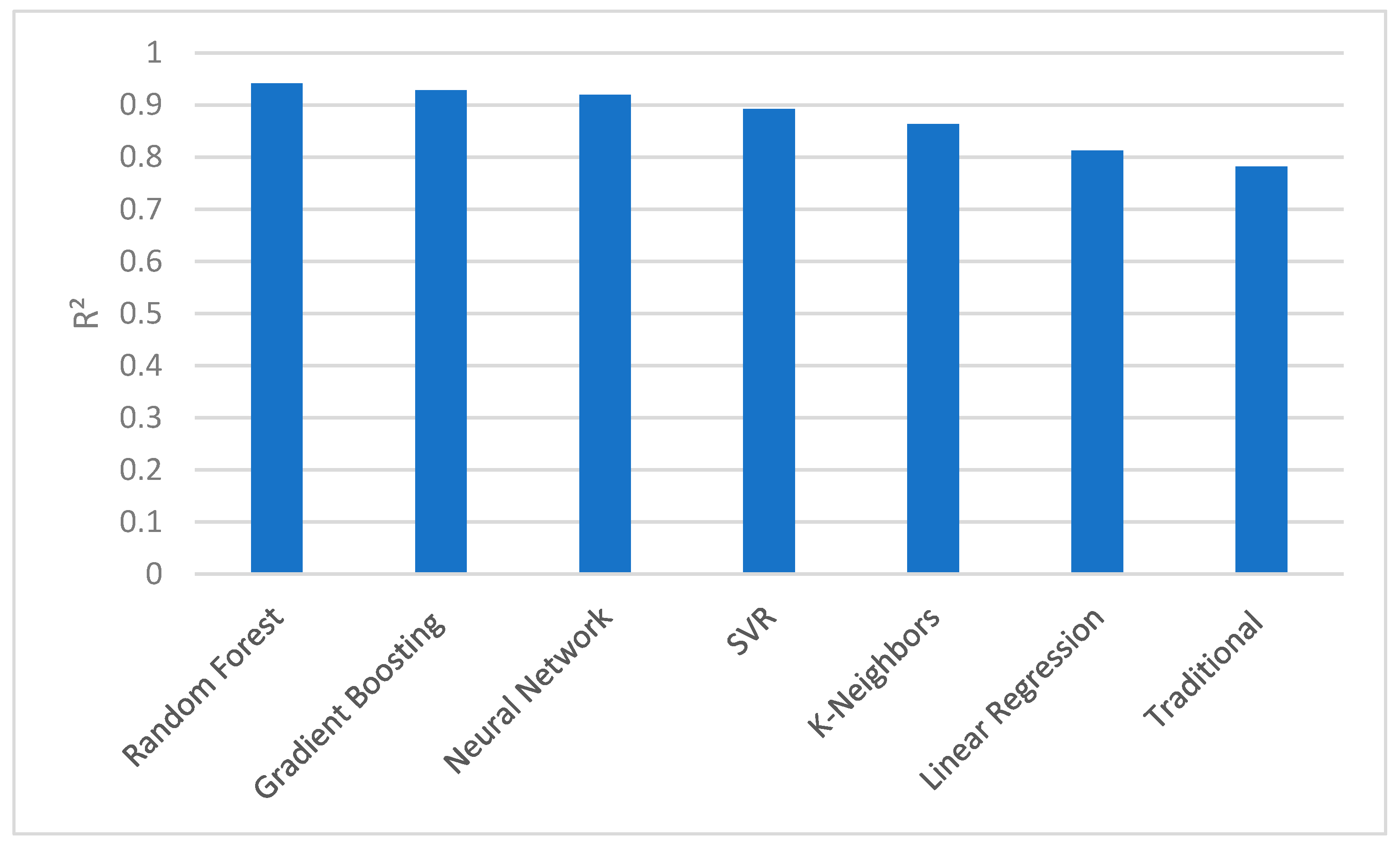
Comparisons of the obtained R² values for all the algorithms are shown in Figure 17. As observed, the maximum R² was yielded by Random Forest at 0.941, closely followed by Gradient Boosting and the ANN. The R² further decreased at a magnitude of 0.892 for SVR, with the lowest magnitude exhibited by Linear Regression at 0.812. Due to better optimization of folds and arrangement of training sets, Random Forest and Gradient Boosting outperformed the SVR and Linear Regression models.

For MPD prediction, the models showed slightly lower performance, reflecting the inherent challenges in predicting profile-based measurements from surface data. Regarding MPD prediction performance, Random Forest, again, outperformed other models, with R² = 0.917 and MAE = 0.058 mm, though with slightly lower overall accuracy compared with MTD prediction, exhibiting the inherent challenges in predicting profile-based measurements from surface data, as shown in

Table 11. MPD prediction performance comparison.

Model	R2	MAE (mm)	RMSE (mm)	MAPE (%)
Random Forest	0.917	0.058	0.076	7.84
Gradient Boosting	0.904	0.063	0.082	8.52
ANN	0.893	0.069	0.088	9.31
SVR	0.871	0.078	0.097	10.67
KNN	0.842	0.091	0.113	12.45
Linear Regression	0.798	0.107	0.132	14.82

.

6.6. Cross-Validation of Results

The stability and generalization capability of the models were assessed through five-fold cross-validation. The cross-validation results across five folds show the consistency and stability of model performances with low standard deviations, particularly for Random Forest (0.941 ± 0.006), indicating a reliable generalization capability, with the least performance exhibited by KNN, as shown in

Table 12. Cross-validation results.

Model	Fold 1 R2	Fold 2 R2	Fold 3 R2	Fold 4 R2	Fold 5 R2	Mean R2	Std. Dev.
Random Forest	0.938	0.945	0.932	0.947	0.941	0.941	0.006
Gradient Boosting	0.925	0.931	0.919	0.934	0.928	0.927	0.006
ANN	0.915	0.923	0.908	0.926	0.919	0.918	0.007
SVR	0.888	0.897	0.882	0.895	0.892	0.891	0.006
KNN	0.858	0.867	0.851	0.865	0.863	0.861	0.006

.

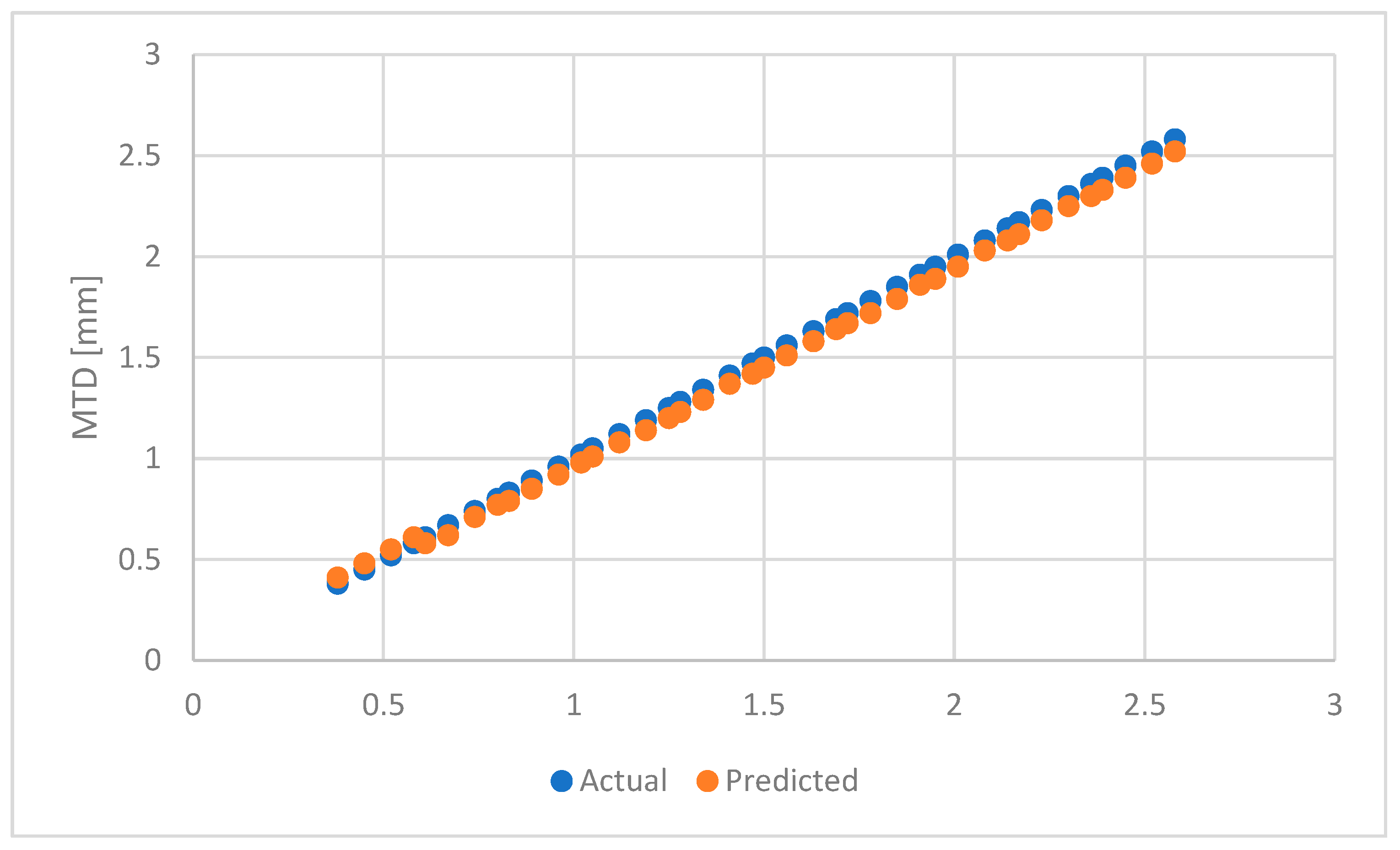
Since the highest R² was shown by Random Forest, the graph showing the comparison of actual values obtained using the sand patch method and predicted values using the Random Forest algorithms is shown in Figure 18. As observed, the predicted values were overestimated in the first four instances of observations, and it slowly started slightly underestimating the predicted values until the end of observation for 0.7 mm, exhibiting underestimation of observations, and as the data population increased, the predicted values were overestimated, with an MTD over 0.7 mm by Random Forest algorithms.

6.7. Error Analysis

The distribution of prediction errors was analyzed to understand model behavior across different texture depth ranges. The error distribution analysis is shown in

Table 13. Error distribution across MTD ranges.

MTD Range (mm)	Samples	Mean Error (mm)	Std. Dev. (mm)	Max. Error (mm)
0.25–0.75	28	0.042	0.031	0.098
0.75–1.25	35	0.058	0.042	0.134
1.25–1.75	29	0.071	0.053	0.187
1.75–2.25	19	0.089	0.067	0.223
2.25–2.75	11	0.104	0.078	0.261
2.75–3.45	5	0.127	0.095	0.298

. It consists of the prediction accuracy across different MTD ranges, revealing that the error magnitude increased with texture depth, from an MAE of 0.042 mm for smooth surfaces (MTD: 0.25–0.75 mm) to an MAE of 0.127 mm for very rough surfaces (MTD: 2.75–3.45 mm), providing important insights into model behavior across varying conditions. The observed degradation in the prediction accuracy for surfaces with an MTD exceeding approximately 2.7 mm was due to two fundamental, interrelated limitations inherent to the integrated sensor model system. Firstly, the 3D-structured light scanner encountered a physical boundary condition on such extremely rough surfaces. Deep voids and sharp aggregate edges created significant occlusions and shadows that the scanner’s projected light pattern could not fully penetrate, leading to a systematic undersampling of the deepest texture features. The resulting point cloud represented a geometrically filled-in version of the true surface. Secondly, this data limitation was compounded by the statistical distribution of the training data. The dataset included samples of up to 3.45 mm. The natural scarcity of extremely high MTD surfaces limited the model to learn the complex and high-variance geometric signatures associated with severe texture. Therefore, the model operated near the boundary of its learned feature space, performing a less reliable form of extrapolation. This performance boundary does not invalidate the model, but it defines its optimal operational range, which can be further refined through techniques like multi-sensor fusion and domain-specific sub-modeling.

The machine learning approach demonstrated several significant advantages over traditional methods in terms of speed, accuracy, consistency, and scalability, with a detailed comparison shown in

Table 14. Comprehensive method comparison.

Aspect	Traditional Sand Patch	Digital Correlation	ML Prediction
Accuracy (MAE)	0.000 mm (reference)	0.152 mm	0.067 mm
Measurement time	15–20 min	2–3 min	<5 sec
Labor required	High	Medium	Low
Equipment cost	Low	High	High
Skill required	High	Medium	Low
Repeatability	Medium	High	Very high
Scalability	Low	Medium	High

. A comprehensive comparison is shown between traditional sand patch testing, digital correlation methods, and the proposed machine learning approach across multiple practical dimensions, including accuracy, measurement time, labor requirements, equipment cost, and scalability, demonstrating the significant advantages of the machine learning method in terms of speed (under 5 s vs. 15–20 min), accuracy (0.067 mm vs. 0.152 mm MAE), and scalability while acknowledging the higher initial equipment cost requirement.

The accuracy of digital measurement depends on the number of points per unit area; however, it can be observed among samples showing very close correlation that the sets with the highest point density did not always give the best result, but, rather, a ratio characterized by a surface/point density ratio. One of the main directions for the technology’s development is the optimization of point density, as this significantly affects not only the model’s accuracy but also its creation time, which requires excessively large computational capacity for unnecessarily high accuracy.

7. Conclusions and Findings

This research established a methodology for pavement macrotexture assessment by integrating 3D laser-scanning technology with advanced machine learning algorithms. This study demonstrated that machine learning models can transcend the limitations of traditional linear correlations, achieving a higher level of accuracy. The core finding of this work is the superior predictive performance of ensemble methods, with the Random Forest algorithm emerging as the most effective model for predicting MTD. This model achieved a coefficient of determination R² of 0.941 and a mean absolute error (MAE) of 0.067 mm, which represents a 56% improvement in accuracy over conventional digital correlation methods. Therefore, pavement texture is not defined by a single geometric property; however, it is a multifactorial characteristic influenced by a combination of height distribution, spatial arrangement, and volumetric properties.

The comprehensive feature engineering process, which extracted 27 distinct parameters from the 3D point cloud data, was fundamental to the model’s performance. The analysis revealed that the most influential features for predicting texture depth were the root mean square height (Sq), surface skewness (Ssk), and developed interfacial area ratio (Sdr). This indicates that accurate texture characterization requires considering both the amplitude of surface variations and the complexity of the spatial distribution. The comparative evaluation of six different machine learning algorithms provided clear evidence that ensemble methods like Random Forest and Gradient Boosting are exceptionally well-suited for this task. Their inherent capabilities for handling non-linear relationships, mitigating overfitting, and ranking feature importance made them outperform other algorithms, including Neural Networks, which required greater computational resources for marginally lower results. This research demonstrated an improvement in operational efficiency. The machine learning method reduced the measurement time from 15–20 min per sample for the traditional sand patch test to under 5 s for a prediction, enabling rapid, high-frequency texture assessment.

The practical validity of the developed models was further reinforced through the extended validation study comparing the results with the Dynatest RSP measuring beam. The machine learning-predicted MTD values showed a 98.71% agreement with the estimated texture depth (ETD) derived from the RSP’s MPD measurements, providing an independent measure of the model’s reliability. This correlation also bridges the gap between static, high-resolution scanner data by high-speed profilers, suggesting potential for cross-calibration and data fusion in future pavement management systems. Moreover, this research also identified certain limitations and boundaries. The prediction accuracy was observed to decrease slightly with increasing texture depth, as very rough surfaces present more complex geometries that are inherently more challenging to model. Furthermore, while the models showed excellent generalization across the pavement types included in this study, their performance on entirely new surface materials requires further validation and potential model retraining.

Analysis of the model’s performance across the four pavement types revealed consistent but not uniform accuracy. The Random Forest model achieved the best results for all materials; a measurable difference in the prediction error was observed. Specifically, the model performed slightly better on dense graded asphalt, with an MAE of 0.068 mm, than on porous asphalt, with an MAE of 0.089 mm. This variation is attributed to the fundamental differences in surface morphology between these materials. Porous asphalt has a high void content, resulting in a surface with deeper cavities, with a broader range of texture depths and a more complex, irregular geometry compared with the denser, uniform surface of dense graded asphalt. This finding demonstrates that the prediction precision is influenced by the specific textural characteristics of the material being assessed.

This research provides a machine learning platform that can accurately predict critical texture parameters, including MTD and MPD, from 3D scanner data. It offers a pathway to automate a traditionally labor-intensive and variable process. Future work will focus on expanding the model’s applicability to a wider range of pavement materials and deterioration stages, exploring direct prediction from point clouds, and integrating the prediction into real-time and mobile scanning systems for automated infrastructure condition assessment.

Therefore, using the machine learning algorithms further improved the prediction accuracy when compared with both the sand patch method and the 3D scanner. The machine learning algorithms provide an alternative to predict data with the least error and a reduced computation time. The datasets obtained from laser scanning can be used to train various types of machine learning algorithms, leading to better accuracy in prediction of MTD and MPD. The key findings are as follows.

• Random Forest achieved the best performance, with R² = 0.941 and MAE = 0.067 mm.
• A 56% improvement in accuracy over traditional correlation methods was obtained using machine learning algorithms.
• The prediction time reduced from 15–20 min to under 5 s using the machine learning algorithms.
• Feature importance analysis revealed Sq (RMS height) as the most significant predictor.

References

- Pranjić, I.; Deluka-Tibljaš, A.; Cuculić, M.; Šurdonja, S. Influence of Pavement Surface Macrotexture on Pavement Skid Resistance. Transp. Res. Procedia 2020, 45, 747–754. [Google Scholar] [CrossRef]
- Čelko, J.; Kováč, M.; Kotek, P. Analysis of the Pavement Surface Texture by 3D Scanner. Transp. Res. Procedia 2016, 14, 2994–3003. [Google Scholar] [CrossRef]
- Chen, S.; Liu, X.; Luo, H.; Yu, J.; Chen, F.; Zhang, Y.; Ma, T.; Huang, X. A State-of-the-Art Review of Asphalt Pavement Surface Texture and Its Measurement Techniques. J. Road Eng. 2022, 2, 156–180. [Google Scholar] [CrossRef]
- De Blasiis, M.R.; Di Benedetto, A.; Fiani, M. Mobile Laser Scanning Data for the Evaluation of Pavement Surface Distress. Remote Sens. 2020, 12, 942. [Google Scholar] [CrossRef]
- Aytekin, Ö.; Zongur, U.; Halici, U. Texture-Based Airport Runway Detection. IEEE Geosci. Remote Sens. Lett. 2013, 10, 471–475. [Google Scholar] [CrossRef]
- Naser, M.Z. Interpretable Machine Learning for the Analysis, Design, Assessment, and Informed Decision Making for Civil Infrastructure; Elsevier: Amsterdam, The Netherlands, 2023; pp. 1–283. [Google Scholar] [CrossRef]
- Zhong, J.; Jiang, X.; Cheng, Z.; Xie, S.; Huang, K.; Ma, Y.; Huang, B. Comprehensive Evaluation Framework for Long-Term Pavement Skid Resistance and Texture Evolution. Case Stud. Constr. Mater. 2025, 23, e05474. [Google Scholar] [CrossRef]
- Bitelli, G.; Simone, A.; Girardi, F.; Lantieri, C. Laser Scanning on Road Pavements: A New Approach for Characterizing Surface Texture. Sensors 2012, 12, 9110–9128. [Google Scholar] [CrossRef] [PubMed]
- Mataei, B.; Nejad, F.M.; Zakeri, H. Automatic Pavement Texture Measurement Using a New 3D Image-Based Profiling System. Measurement 2022, 199, 111456. [Google Scholar] [CrossRef]
- Yang, G.; Wang, K.C.P.; Li, J.Q.; Wang, G. A Novel 0.1 Mm 3D Laser Imaging Technology for Pavement Safety Measurement. Sensors 2022, 22, 8038. [Google Scholar] [CrossRef]
- Yaacob, H.; Hassan, N.A.; Hainin, M.R.; Rosli, M.F. Comparison of Sand Patch Test and Multi Laser Profiler in Pavement Surface Measurement. J. Teknol. 2014, 70, 103–106. [Google Scholar] [CrossRef]
- Uz, V.E.; Gökalp, İ. Comparative Laboratory Evaluation of Macro Texture Depth of Surface Coatings with Standard Volumetric Test Methods. Constr. Build. Mater. 2017, 139, 267–276. [Google Scholar] [CrossRef]
- Akraym, H.M.; Muniandy, R.; Jakarni, F.M.; Hassima, S. Texture Depth Measurement Using a Micro-Volume Measurement Technique for Gyratory Compactor Specimens. Open Civ. Eng. J. 2023, 17, e18741495272555. [Google Scholar] [CrossRef]
- Wang, T.; Chu, L.; Fwa, T.F. Improved Numerical Method for Determination of Pavement Mean Texture Depth from 3-Dimensional Digital Image. Constr. Build. Mater. 2022, 358, 129447. [Google Scholar] [CrossRef]
- Chen, B.; Xiong, C.; Li, W.; He, J.; Zhang, X. Assessing Surface Texture Features of Asphalt Pavement Based on Three-Dimensional Laser Scanning Technology. Buildings 2021, 11, 623. [Google Scholar] [CrossRef]
- Tamagusko, T.; Gomes Correia, M.; Ferreira, A. Machine Learning Applications in Road Pavement Management: A Review, Challenges and Future Directions. Infrastructures 2024, 9, 213. [Google Scholar] [CrossRef]
- Zheng, L.; Xiao, J.; Wang, Y.; Wu, W.; Chen, Z.; Yuan, D.; Jiang, W. Deep Learning-Based Intelligent Detection of Pavement Distress. Autom. Constr. 2024, 168, 105772. [Google Scholar] [CrossRef]
- Shi, W.; Niu, D.; Li, Z.; Niu, Y. Effective Contact Texture Region Aware Pavement Skid Resistance Prediction via Convolutional Neural Network. Comput. Civ. Infrastruct. Eng. 2024, 39, 2054–2070. [Google Scholar] [CrossRef]
- Liu, X.; Yin, C. 3D Reconstruction of Asphalt Pavement Macro-Texture Based on Convolutional Neural Network and Monocular Image Depth Estimation. Appl. Sci. 2025, 15, 4684. [Google Scholar] [CrossRef]
- Wan, X.; Yu, X.; Chen, M.; Ye, H.; Liu, Z.; Yu, Q. Prediction of Skid Resistance of Asphalt Pavements on Highways Based on Machine Learning: The Impact of Activation Functions and Optimizer Selection. Symmetry 2025, 17, 1708. [Google Scholar] [CrossRef]
- Taheri, A.; Sobanjo, J. Ensemble Learning Approach for Developing Performance Models of Flexible Pavement. Infrastructures 2024, 9, 78. [Google Scholar] [CrossRef]
- Azam, A.; Alshehri, A.H.; Alharthai, M.; El-banna, M.M.; Yosri, A.M.; Beshr, A.A.A. Applications of Terrestrial Laser Scanner in Detecting Pavement Surface Defects. Processes 2023, 11, 1370. [Google Scholar] [CrossRef]
- Kováč, M.; Brna, M.; Pisca, P.; Jandačka, D.; Decký, M. The Influence of Road Pavement Materials on Surface Texture and Friction. Sustainability 2023, 15, 12195. [Google Scholar] [CrossRef]
- Zhao, L.; Zhang, H.; Mbachu, J. Multi-Sensor Data Fusion for 3D Reconstruction of Complex Structures: A Case Study on a Real High Formwork Project. Remote Sens. 2023, 15, 1264. [Google Scholar] [CrossRef]
- Weng, Z.; Xiang, H.; Lin, Y.; Liu, C.; Wu, D.; Du, Y. Pavement Texture Depth Estimation Using Image-Based Multiscale Features. Autom. Constr. 2022, 141, 104404. [Google Scholar] [CrossRef]
- Bai, J.; Wu, D.; Shelley, T.; Schubel, P.; Twine, D.; Russell, J.; Zeng, X.; Zhang, J. A Comprehensive Survey on Machine Learning Driven Material Defect Detection. ACM Comput. Surv. 2025, 57, 1–36. [Google Scholar] [CrossRef]
- Dan, H.C.; Lu, B.; Li, M. Corrigendum to “Evaluation of Asphalt Pavement Texture Using Multiview Stereo Reconstruction Based on Deep Learning” [Constr. Build. Mater. 412 (2024) 134837]. Constr. Build. Mater. 2025, 481, 141630. [Google Scholar] [CrossRef]
- Lu, B.; Lu, Z.; Qi, Y.; Guo, H.; Sun, T.; Zhao, Z. Predicting Asphalt Pavement Friction by Using a Texture-Based Image Indicator. Lubricants 2025, 13, 341. [Google Scholar] [CrossRef]
Figure 1.
Research methodology.
Figure 2.
Cleaning of pavement surface.
Figure 3.
Measurement of replacement sand.
Figure 4.
Arctec Space Spider scanner.
Figure 5.
Assembling the measuring system.
Figure 6.
Complete scanning setup.
Figure 7.
Raw version of scanned surfaces.
Figure 8.
Conversion to 3D patch.
Figure 9.
Conversion to 30 cm diameter patch.
Figure 10.
Three-dimensional point cloud generation in CloudCompare software.
Figure 11.
Segmentation for point cloud data.
Figure 12.
Comparison of scanner and sand patch values for whole section.
Figure 13.
Comparison of scanner and sand patch values for 30 cm diameter at lower texture depth.
Figure 14.
Comparison of scanner and sand patch values after enhancing dataset.
Figure 15.
Comparison of scanner and sand patch values for 30 cm diameter after enhancing dataset.
Figure 16.
Top 10 features by importance.
Figure 17.
Graphical representation of R2 values.
Figure 18.
Actual vs. predicted MTD values for Random Forest.