Developing a Regionally Adaptable CPT-SPT Correlation Using Linear Regression and Genetic Algorithms

Abstract

Establishing a correlation between the Cone Penetration Test (CPT) and the Standard Penetration Test (SPT) is of significant importance for geotechnical engineering practice. A novel correlation between CPT-q_t and SPT-N₆₀ based on a genetic algorithm (GA) and linear regression was proposed in this study. Based on the soil behavior type index (I_c), a GA was first applied to divide the dataset into different I_c intervals. Subsequently, linear regression was performed separately for the data in each interval to establish a correlation between CPT-q_t and SPT-N₆₀. Concurrently, the Segmented Information Criterion (SIC) was introduced to perform dual-objective optimization of complexity and prediction accuracy. The results indicate that the proposed model achieved an R² of 0.60 and an RMSE of merely 8.10. Specifically, the R² values improved by 33% and 5% compared to the traditional models and the AI models, respectively. On the validation dataset, the proposed model achieved an R² of 0.67 and an RMSE of 4.33, demonstrating higher accuracy compared to the traditional models. In summary, a method for investigating the CPT-SPT correlation is proposed in this study, characterized by simplicity, efficiency, and enhanced reliability. Additionally, a novel criterion (SIC) for mitigating overfitting is introduced. These two research findings can provide more reliable input parameters for SPT-based design, thereby supporting geotechnical engineering applications, and offer a valuable reference for relevant studies in other regions.

1. Introduction

The Standard Penetration Test (SPT) is a widely used method for evaluating the geotechnical properties of soil layers. During the test, a 63.5 kg hammer is freely dropped from a height of 76 cm to drive a standard split-spoon sampler into the soil stratum. The penetration process is divided into three consecutive 30 cm increments, with the sum of blow counts recorded during the second and third 30 cm increments defined as the “N-value”. However, the N-value may be influenced by multiple factors, including the rod length and energy transfer efficiency during testing. Therefore, the raw N-value should be corrected to a normalized value. This corrected value is designated as N₆₀, calculated as follows:

$$N_{60}=N\times \left({ER}_r/60\right)$$

(1)

where ${ER}_r$ is the rod energy ratio of the methodology [1,2].

The in situ engineering properties of soil strata are primarily evaluated through the SPT, with relatively undisturbed samples being collected for subsequent laboratory testing. The SPT has become a widely adopted in situ testing method for geotechnical field investigations. A wide range of soil-related geotechnical design parameters have been derived from the SPT, and extensive empirical relationships have been established based on SPT results, which serve as guidance for geotechnical design and engineering practice [3].

The Cone Penetration Test (CPT) is an accurate and efficient in situ testing method commonly used for obtaining continuous soil profiles. During the test, a cone-shaped probe is advanced into the ground at a constant rate of approximately 2 cm/s while the cone tip resistance (q_c), sleeve friction (f_s), and pore water pressure (u) are recorded. The specific testing procedures are described in ASTM D5778 (2020) [4]. In soft clays and silts, as well as in over-water operations, the measured q_c must be corrected for the effect of pore water pressure to obtain the corrected cone tip resistance (q_t), which is calculated as follows:

$$q_t=q_c+u_2\times \left(1-a\right)$$

(2)

where $u_2$ is the pore water pressure at the base of the sleeve, and $a$ is a parameter obtained through laboratory calibration, typically ranging from 0.70 to 0.85. For sandy soils, q_c is equal to q_t [5].

Due to its high reliability, excellent repeatability, standardized testing procedures, and the ability to rapidly and conveniently obtain continuous soil profiles, the CPT is increasingly becoming a preferred method for geotechnical investigations. However, the relatively high cost limits its application in certain locations [6,7]. In contrast to the CPT, the SPT is simple and low-cost. However, it is highly influenced by human operation and soil heterogeneity, resulting in significant data dispersion and low repeatability, and it is difficult to obtain reliable data in very soft soil layers [8].

Establishing correlations between the CPT and SPT is significant. Many of the empirical relationships in geotechnical engineering and reference values in design applications are based on the SPT. If a reliable correlation can be established, CPT results can utilize existing SPT-based formulas [3]. Additionally, the CPT offers excellent repeatability and data continuity. Its precise correlation model effectively compensates for the limitations of the SPT, such as high result variability and data discontinuity. Overall, in practical applications, such correlation compensates for the respective limitations of both methods while fully leveraging their advantages, thereby providing more reliable and cost-effective solutions for regional geotechnical site investigation and design.

2. Background

It was initially discovered that a simple proportional correlation exists between SPT-N and CPT-q_c. According to Meyerhof (1965) [9], the following correlation applies to all soil types:

$$N=q_c/n$$

(3)

where $n$ equals to 0.4, with q_c expressed in MPa and $N$ in blows.

However, researchers stated that the value of $n$ in the equation varies with soil type. This suggests that the CPT-SPT correlation may vary with changes in soil conditions. For example, Schmertmann (1970) [10] indicated that the value of $n$ ranges from 0.2 to 0.4 for silts, sandy silts, and slightly cohesive silt–sand mixtures; from 0.3 to 0.5 for clean fine to medium sands and slightly silty sands; from 0.4 to 0.5 for coarse sands and sands with little gravel; and from 0.6 to 0.8 for sandy gravel and gravel. And researchers such as Danziger and Velloso (1995), Akca (2003), Kara and Gündüz (2010), Zhao and Cai (2015), and Alam et al. (2018) have also conducted in-depth studies and developed proportional equations between SPT-N and CPT-q_c for different soil types [3,11,12,13,14].

Meanwhile, some researchers have introduced linear equations based on the proportional relationship, attempting to improve the accuracy of the correlation by adding an intercept (Kara and Gündüz (2010), Shahri et al. (2014), Jarushi et al. (2015), and Hossain et al. (2024)) [12,15,16,17]. For example, Akca (2003) established some equations, as presented in Table 1 [3].

Table 1. q_c/N correlation equation for different soil types by Akca (2003) [3].

Soil Type	Correlation
Sand	$N=3.13\times q_c-25.72$
Silty sand	$N=2.27\times q_c-11.57$
Sandy silt	$N=3.57\times q_c-6.25$

In addition, some researchers have suggested that the correlation between the SPT and CPT can be expressed as a function of the median grain size (D₅₀) of the soil [18]. However, D₅₀ is typically obtained through particle size analysis tests, which require additional effort and cost, and the lab results may also be affected by insufficient sample representativeness and laboratory operational errors. Jefferies and Davies (1993) [19] were the first to propose the concept of the soil behavior type index (I_c), which enables continuous characterization of soil types and thus eliminates the need for soil sampling. Robertson and Wride (1998) [20] modified the definition of I_c:

$$I_c={\left[{\left(3.47-\log Q\right)}^2+{\left(\log F+1.22\right)}^2\right]}^{0.5}$$

(4)

where Q and F are calculated as follows:

$$Q=\left(q_t-{\sigma }_{vo}/Pa\right)\times {\left(Pa/{{\sigma }^{\prime }}_{vo}\right)}^n$$

(5)

$$F=\left[f_s/\left(q_t-{\sigma }_{vo}\right)\right]\times 100\%$$

(6)

where ${\sigma }_{vo}$ is the total overburden stress, and ${{\sigma }^{\prime }}_{vo}$ is the effective overburden stress. Since q_t is expressed in MPa, $Pa$ is taken as 0.1 MPa.

Lunne et al. (1997) [21] adopted the definition of I_c given in Equation (4) and established a correlation between the SPT-N and CPT:

$$\left(q_c/Pa\right)/N_{60}=0.85\times \left(1-I_c/4.6\right)$$

(7)

Robertson (2012) [22] updated the correlation in Equation (7):

$$\left(q_c/Pa\right)/N_{60}={10}^{\left(1.1268-0.2817I_c\right)}$$

(8)

In addition to the aforementioned model types, some researchers have also developed other types. In terms of prediction using soil parameters, apart from the commonly used D₅₀, Chin et al. (1990) [23] and Kulhawy and Mayne (1990) [24] proposed SPT–CPT correlations related to the fine content (FC%) in soil samples, while Idriss and Boulanger (2006) [25] proposed correlations associated with the relative density (D_r) of soil. Also, Arifuzzaman and Anisuzzaman (2022) [26] investigated the correlations between f_s and N. Lu et al. (2023) [8] proposed a method for establishing the correlation between the SPT and CPT in sandy soils based on Bayesian theory. Bol (2023) [5] proposed an exponential model based on I_c. And Cheng et al. (2024) [27] developed an SPT-CPT relationship model using the S-curve approach.

In recent years, artificial intelligence (AI) technologies have been developed rapidly, achieving extensive applications particularly in data-driven research domains. An increasing number of researchers are adopting machine learning and deep learning models to explore correlations between the CPT and SPT. Tarawneh (2017) [28] established an artificial neural network (ANN) model for predicting SPT-N₆₀ values based on the CPT. Al Bodour et al. (2022) [29] developed a GEP model with enhanced N₆₀ predictive accuracy. Bai et al. (2024) [30] developed a convolutional neural network (CNN) model to predict the N-value. Mehedi A. Ansary and Mushfika Ansary (2024) [31] applied five different approaches to establish correlations between the SPT and CPT.

However, existing methods each have their limitations: Linear models and empirical formulas typically have narrow applicability and insufficient generalization capabilities in complex geological formations. For instance, some unified predictive functions fail to adequately capture variations in the CPT-SPT correlation under differing geological conditions. Meanwhile, traditional AI models suffer from a black-box nature, which limits their practical application. These limitations highlight the need for methods that are not only statistically robust but also practically adaptable to heterogeneous geological settings.

The objective of this study is to address the aforementioned issues and propose a widely applicable, simple, and reliable research method for establishing the CPT-SPT correlation in engineering practice. First, the advantageous analytical capability of the genetic algorithm (GA) is employed to divide the dataset based on I_c, identifying the linear relationships between N₆₀ and q_t within different I_c ranges. The objective is to employ a data-driven approach to replace empirical methods, thereby assigning data with a similar CPT-SPT correlation to the same interval. Subsequently, linear regression is performed to establish the CPT–SPT correlation between N₆₀ and q_t for each interval. The GA is employed exclusively during the model development phase. Consequently, the final result is presented solely in the form of simple linear models, effectively circumventing the broad applicability challenges associated with conventional black-box machine learning approaches. Moreover, this study introduces a novel Segmented Information Criterion (SIC) to balance model complexity and predictive accuracy, thereby mitigating overfitting and offering a fresh perspective for related research.

3. Datasets

A dataset of 896 CPT-SPT pairs was utilized for model development in this study. These data were collected by Zhou et al. (2021) [32] from 230 locations across the South Island of New Zealand. All paired SPT and CPT data points in the dataset were acquired within 12 m horizontal spacing at each testing location. As CPT measurements are typically recorded at 20 mm depth intervals, each 300 mm SPT interval contains at least 15 CPT measurement points. The arithmetic mean of the CPT values within each 300 mm interval is calculated as the representative value for that interval, which is then paired with the corresponding SPT value. And the q_c was corrected to q_t to account for pore water pressure effects. Figure 1 illustrates the distribution of parameters for the dataset, including q_t, I_c, N₆₀, and (q_t/Pa)/N₆₀. Measurements with q_t values below 20 MPa account for 89% of the total dataset, while 87% of the (q_t/Pa)/N₆₀ ratios are below 10. This indicates the concentration of both parameters in relatively low numerical ranges. The distribution of I_c approximates a normal distribution but exhibits a certain degree of left skewness. For N₆₀, a consistently decreasing pattern is observed across the dataset.

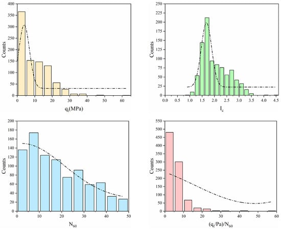
Figure 1. Distribution of q_t, I_c, N₆₀, and (q_t/Pa)/N₆₀ in the original dataset.

Table 2 presents the soil behavior types defined by different I_c values proposed by Robertson (2015) [33], along with the corresponding counts of each soil behavior type in the dataset according to this classification criterion.

Table 2. Summary of soil behavior type in this dataset.

Soil Behavior Type	Ic	Counts
Organic soils—clay	>3.60	2
Clays—silty clay to clay	2.95–3.60	64
Silt mixtures—clayey silt to silty clay	2.60–2.95	100
Sand mixtures—silty sand to sandy silt	2.05–2.60	199
Sands—clean sand to silty sand	1.31–2.05	499
Gravelly sand to dense sand	<1.31	32
Total number of samples	0.86–4.54	896

Preliminary analyses indicate that the dataset in this study exhibits I_c values ranging from 0.86 to 4.54 (as shown in the last row of Table 2), with the dataset being predominantly composed of coarse-grained soils (I_c < 2.60), including silt mixtures, sand mixtures, sands, and gravelly sand to dense sand. Therefore, the proposed model is expected to demonstrate stronger applicability to such soil types.

Identification of outliers is a critical step in data analyses and model construction and is also essential for optimization of model performance. If outliers are not properly filtered before the model construction process, they may adversely affect predictive performance and stability of the model [27,29]. In this study, the box plot method was employed for data screening [34]. Figure 2 visually demonstrates outlier representation within box plots, which characterize data distributions through the lower quartile (Q1), upper quartile (Q3), and median. Data points beyond 1.5 times the interquartile range (IQR, calculated as Q3 − Q1) are considered outliers; specifically, they refer to values below Q1 − 1.5 × IQR or above Q3 + 1.5 × IQR.

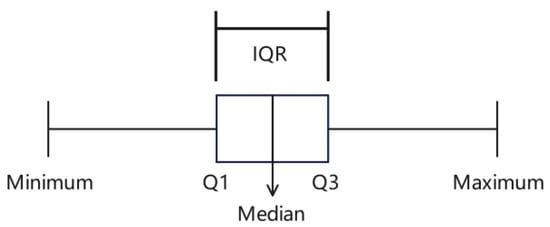
Figure 2. Schematic of box plot method.

(q_t/Pa)/N₆₀ was employed as the screening parameter due to its comprehensive representation of both q_t and N₆₀ distributions in this study [5]. The calculated outlier range was determined as values below −2.96 or exceeding 13.04. Given that (q_t/Pa)/N₆₀ values are inherently positive in practice, only data points exceeding 13.04 were identified and removed. Figure 3 illustrates this outlier screening process, where open circles denote outliers. After the data screening process, 834 validated data pairs were obtained, with 62 data pairs being excluded during screening. These pairs formed the dataset for model development.

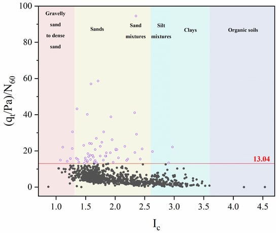
Figure 3. Illustration of data screening process based on the box plot method.

Pearson correlation analyses were performed on the screened dataset to select appropriate features for subsequent linear model development. The Pearson correlation coefficient (r) is a statistical measure used to quantify the degree of linear correlation between two variables, with values ranging from −1 to 1. A value of 1 or −1 indicates an ideal positive or negative linear correlation, respectively, while a value of 0 indicates the non-existence of a linear correlation. In general, an absolute value of |r| greater than 0.70 indicates a strong linear correlation [35]. Figure 4 presents a heatmap of Pearson correlation coefficients among the features in the dataset.

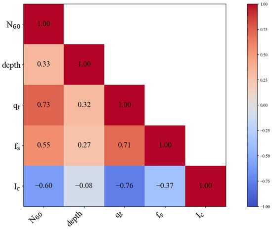
Figure 4. Pearson correlation between CPT and SPT parameters.

In this study, the linear association strengths between each feature (depth, q_t, f_s, and I_c) and the N₆₀ value were systematically evaluated. Pearson correlation analyses revealed that q_t exhibited a correlation coefficient of 0.73 with N₆₀, indicating a significant linear correlation (|r| > 0.7). In contrast, I_c and f_s demonstrated moderate linear correlations with N₆₀, respectively (r = −0.60 and r = 0.55, respectively; 0.5 ≤ |r| < 0.7). Further analyses identified a strong negative correlation between q_t and I_c (r = −0.76) and a strong positive correlation between q_t and f_s (r = 0.71). This implies that including q_t, I_c, and f_s simultaneously as input variables in subsequent linear regression model construction would cause severe multicollinearity, as the information contained in I_c and f_s is largely represented by q_t, resulting in a high degree of overlap in the information among them. Consequently, it becomes difficult to identify the independent contribution of each variable, leading to inaccurate coefficient estimation.

In addition, f_s is generally considered less reliable than q_t [16]. While directly incorporating f_s as an input variable could increase the information content, it may also introduce additional errors, thereby weakening the generalization capability of the proposed model. Therefore, this study employs I_c (calculated from q_t and f_s) as the criterion for data division rather than directly using f_s as an input variable. This approach indirectly utilizes information from f_s while avoiding the direct introduction of its measurement errors into the model.

Therefore, q_t was retained as the sole feature in the model construction. The CPT-SPT correlation within each I_c interval is therefore defined as follows:

$$N_{60}=k\times q_t+b$$

(9)

where $k$ and $b$ are undetermined coefficients that need to be determined through data fitting within each I_c interval.

4. Methodology and Model Development

4.1. Genetic Algorithm (GA)

After completing the preliminary analyses and preprocessing of the dataset, GA was employed as the primary analytical tool to further explore the linear relationships in the data.

GA is an optimization algorithm inspired by the principles of natural selection and genetic mechanisms, and it is widely used to solve complex optimization problems. Figure 5 illustrates the general workflow of the GA [36].

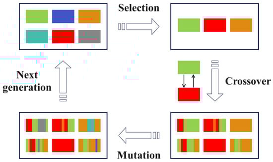
Figure 5. The workflow of the genetic algorithm.

Given the complex soil conditions, the CPT-SPT relationship may exhibit significant variations across different soil types. I_c is a parameter that comprehensively reflects soil characteristics. In this study, the GA is specifically tailored to enhance the prediction of N₆₀. By using the GA to divide the data into different I_c intervals, datasets exhibiting similar CPT-SPT relationships can be maximally grouped within the same I_c interval. Figure 6 illustrates the specific GA workflow implemented in this study, which consists of the following steps:

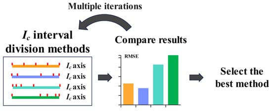
Figure 6. GA-based optimization process for I_c interval division.

• Multiple I_c interval division methods are systematically generated.
• The predictive performance of each method is quantitatively evaluated based on fitting accuracy metrics.
• The I_c interval division method with the lowest prediction errors is identified and selected as the optimal method.

The core parameters of the GA in this study are set as follows: The population size is set to 400 individuals. For selection, the fast non-dominated sorting and crowding distance comparison mechanism from the Non-Dominated Sorting Genetic Algorithm II (NSGA-II) is adopted. The crossover and mutation rates are set to 0.7 and 0.3, respectively. The algorithm terminates after 30 generations, which serves as the stopping criterion. Moreover, the GA ensures the monotonicity of interval boundaries and the non-overlapping nature of intervals through three mechanisms: individual initialization, boundary repair functions, and fitness evaluation. Through this methodology, more precise linear regression models can be developed for each interval.

4.2. Segmented Information Criterion (SIC)

Excessive data divisions may result in insufficient data volume within individual I_c intervals, potentially causing overfitting to the training data that compromises predictive performance on unseen data. Conversely, insufficient divisions fail to adequately capture different linear relationships of the dataset. An overly small number of intervals would result in data within the same I_c interval not necessarily sharing similar relationships, which would in turn reduce the predictive accuracy of the model for N₆₀. Consequently, determining an appropriate number of I_c intervals is important. A dual-objective framework balancing predictive accuracy against model complexity is necessitated, wherein the optimal number of intervals is determined through the identification of an equilibrium point using quantifiable metrics.

In previous studies, the Akaike Information Criterion (AIC) and Bayesian Information Criterion (BIC) are conventionally employed to balance model complexity against predictive performance for optimal model selection [37]. However, these criteria solely penalize the number of parameters in a model rather than being designed to account for division quantity. Consequently, the Segmented Information Criterion (SIC) is proposed as an evaluation metric to balance model complexity and predictive accuracy. Minimizing the SIC indicates an optimal balance between these objectives, with its expression defined as follows:

$$SIC=\alpha \times RMSE+\beta \times m+\gamma \times \sum _{i=1}^m{\displaystyle \frac{1}{n_i}}$$

(10)

where $m$ is the number of I_c intervals, $n_i$ is the number of data points within the i-th I_c interval, and $\alpha$ is the weighting factor for the influence of prediction accuracy, while $\beta$ and $\gamma$ are constraint weights controlling, respectively, the number of intervals and the amount of data in each interval. $\mathsf{\gamma }$ is incorporated to ensure adequate data points in each interval.

And the Root Mean Square Error (RMSE), a statistical metric quantifying prediction error magnitude, is calculated as follows:

$$RMSE =\sqrt{{\displaystyle \frac{1}{n}}\sum _{i=1}^n{(y_i-\widehat{y_i})}^2}$$

(11)

where $n$ is the total number of data points, which equals 834 in this study. $y_i$ is the actual value, and $\widehat{y_i}$ is the predicted value of the model. A smaller RMSE value indicates higher prediction accuracy of the model, whereas a larger RMSE value reflects lower prediction accuracy.

The determination of the weighting coefficients $\alpha$, $\beta$, and $\gamma$ governs the number of I_c intervals in model development. Initially, normalization is applied to the RMSE, the number of intervals m, and $\sum _{i=1}^m{\displaystyle \frac{1}{n_i}}$ to ensure these three features are evaluated on a unified scale. Normalization is a linear transformation process where the minimum value is scaled to 0, the maximum to 1, with all other values proportionally distributed between 0 and 1, with the formula defined as follows:

$$X^{\prime }={\displaystyle \frac{X-X_{\mathit{min}}}{X_{\mathit{max}}-X_{\mathit{min}}}}$$

(12)

where $X^{\prime }$ is the normalized data, $X$ is the original data, and $X_{\mathit{max}}$ and $X_{\mathit{min}}$ are the maximum and minimum values in the dataset, respectively. $X_{\mathit{max}}-X_{\mathit{min}}$ functions as the scaling factor utilized to transform the original data range to [0,1].

Following the normalization of the initial data of these three features, through empirical analysis and repeated trials, the values assigned to ${\alpha }_{standard}$, ${\beta }_{standard}$, and ${\gamma }_{standard}$ for the normalized RMSE, m, and $\sum _{i=1}^m{\displaystyle \frac{1}{n_i}}$ are determined as 1, 2, and 1, respectively.

The values of ${\alpha }_{standard}$, ${\beta }_{standard}$, and ${\gamma }_{standard}$ are based on the normalized data of the RMSE, m, and $\sum _{i=1}^m{\displaystyle \frac{1}{n_i}}$. To ensure interpretability within the original data dimensions, these normalized features must be inversely transformed back to their native scales prior to SIC computation. Concurrently, the standardized parameters ${\alpha }_{standard}$, ${\beta }_{standard}$, and ${\gamma }_{standard}$ are rescaled according to the respective scaling factors of the RMSE, m, and $\sum _{i=1}^m{\displaystyle \frac{1}{n_i}}$ to align with native data dimensions. For instance, the scaling factor conversion for $\alpha$ and the RMSE is implemented as follows:

$${Scale}_{RMSE}={RMSE}_{max}-{RMSE}_{min}$$

(13)

where ${Scale}_{RMSE}$ is the scaling factor for the RMSE during data normalization, and ${RMSE}_{max}$ and ${RMSE}_{min}$ are the maximum and minimum values of the RMSE in the original dataset, respectively.

Therefore, $\alpha$ is computed for the native-scale RMSE as follows:

$$\alpha ={\alpha }_{standard}\times {Scale}_{RMSE}$$

(14)

The values of $\alpha$, $\beta$, and $\gamma$ are determined as 1.08, 0.07, and 0.75, respectively. Consequently, the formulation of SIC in this study is defined as follows:

$$SIC=1.08\times RMSE+0.07\times m+0.75\times \sum _{i=1}^m{\displaystyle \frac{1}{n_i}}$$

(15)

Following the determination of the SIC computational framework, the dataset was initially divided into m I_c intervals with equivalent initial data volumes, where m denotes the predefined number of intervals. Starting from initial I_c interval boundaries, iterative optimization was performed where each cycle was dedicated to group CPT-SPT data with similar linear relationships into identical I_c intervals. All possible interval division schemes were comprehensively explored, and the I_c boundaries that yielded the highest N₆₀ prediction accuracy were determined.

Figure 7 presents the RMSE between the estimated and measured N₆₀ values for the entire dataset under each predefined number (m) of intervals, as well as the SIC computation results obtained under the corresponding division conditions.

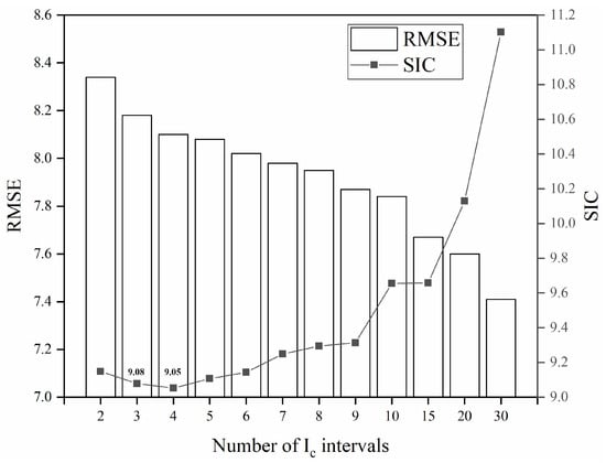
Figure 7. Comparison of RMSE and SIC for different number of I_c intervals.

As illustrated in Figure 7, finer data division corresponds to a lower RMSE, indicating reduced prediction errors. This demonstrates a positive correlation between the number of I_c intervals and the prediction accuracy of the model. However, the lowest SIC value of 9.05 was achieved at four intervals, indicating an optimal balance between model complexity and predictive accuracy. This indicates that exceeding four I_c intervals leads to overfitting in the established model. In another words, although the models constructed by dividing the data into more than four I_c intervals may achieve higher N₆₀ prediction accuracy on data from the South Island of New Zealand, their predictive capability in datasets from other regions will conversely be lower. In Section 4.3, data from other regions were utilized to validate the reliability of the SIC.

4.3. Validation of the SIC

To validate the effectiveness of the SIC in mitigating model overfitting, in-depth analyses were conducted using 42 sets of CPT-SPT data from two other regions [5,37] in this study. The new dataset was not used in the model development process described in Section 4.2. The distribution characteristics of the parameters in the newly used dataset are presented in Table 3.

Table 3. Statistical characteristics of the new dataset for validation.

Soil Behavior Type	Counts	Variables	Maximum	Minimum	Means	Standard Deviation
Sands	10	qt (MPa)	27.30	4.11	10.03	6.87
		Ic	1.93	1.44	1.69	0.17
		N60	36.85	10.00	16.34	8.20
Sand mixtures	2	qt (MPa)	3.62	3.51	3.57	0.08
		Ic	2.44	2.06	2.25	0.27
		N60	9.45	9.40	9.43	0.04
Silt mixtures	10	qt (MPa)	3.15	0.63	1.43	0.92
		Ic	2.89	2.63	2.79	0.09
		N60	20.00	0.92	7.62	7.21
Clays	20	qt (MPa)	1.64	0.31	0.70	0.34
		Ic	3.35	2.95	3.12	0.12
		N60	15.00	1.00	4.65	3.91

Since models with different numbers of I_c intervals have already been established in Section 4.2, these models were validated using the new dataset in this section. Specifically, the models developed based on South Island of New Zealand data are applied to the new datasets for N₆₀ prediction. To comprehensively assess the capability of the models, the R² metric is introduced. R² is a statistical measure that represents the proportion of the variance in the dependent variable that is explained by the independent variables, serving as an essential indicator of the robustness of a regression model. Generally, the closer the R² value is to 1, the better the model fits the data. It can be calculated using the following equation:

$$R^2=1-{\displaystyle \frac{{\sum }_{i=1}^n{\left(y_i-\widehat{y_i}\right)}^2}{{\sum }_{i=1}^n{\left(y_i-\overline{y_i}\right)}^2}}$$

(16)

where $n$ is the total number of data points, $y_i$ is the measured values, $\widehat{y_i}$ is the estimated values, and $\overline{y_i}$ is the mean of all measured values.

By comparing the R² and RMSE of each model, the model with the best prediction accuracy on data from other regions can be identified. Specifically, models established in Section 4.2 by dividing the data into 2 to 30 I_c intervals were validated using unseen data. If the model constructed with four I_c intervals achieves the highest prediction accuracy, it will demonstrate the effectiveness of the SIC.

Figure 8 presents a comparison between the estimated and measured values from the models with different numbers of intervals. Since the R² of the models established with more than five I_c intervals gradually decreases on the new dataset, only the models built under the first four division scenarios are shown in Figure 8 for comparison.

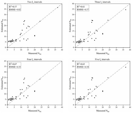
Figure 8. Comparison of predictive accuracy among different models with different numbers of I_c intervals.

It can be observed that the model built with four I_c intervals achieves the best predictive performance on the data from other regions, with an R² of 0.67. This validates the effectiveness of the SIC in mitigating model overfitting. Due to the limited size of the validation dataset, the SIC coefficient values may require further optimization for application in other regions.

4.4. Model Development

Based on the findings in Section 4.3, this section will elaborate on the model construction process for I_c division into four intervals, as described in Section 4.2.

Figure 9 reveals a significant decline in the RMSE during initial iterations, indicating rapid error convergence in the early optimization phase. Beyond the 8th iteration, the RMSE curve was observed to be flat with diminished fluctuation magnitude, and the change in the RMSE was less than 0.1%, demonstrating the approach to optimization stability.

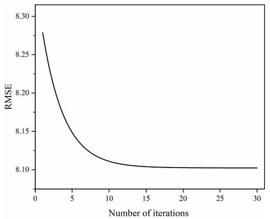
Figure 9. Variation in RMSE during GA iterations.

Figure 10 documents the evolutionary transition from initial to final I_c boundary values. In Figure 10a, the primary objective of the initial equal-interval division method is to achieve mathematical simplicity. Ultimately, when the I_c intervals are defined as [0.860, 1.426, 1.858, 2.212, 4.540], the model achieves its minimum RMSE of 8.10. In Figure 10b, the number of data points in the I_c range of [1.426, 1.858] is 348, which is the largest, while that in the interval [0.860, 1.426] is 59, which is the smallest. The variation in the number of data points across the optimized I_c intervals is an expected and intentional outcome of the GA optimization process. Intervals that exhibit a strong and consistent linear relationship (e.g., [1.426, 1.858]) are expanded to incorporate more homogenous data points, resulting in a higher count. Conversely, intervals with weaker or more scattered correlations (e.g., [0.860, 1.426]) are reduced to isolate a more consistent division, leading to fewer data points. This data imbalance reflects the complexity of actual soil conditions.

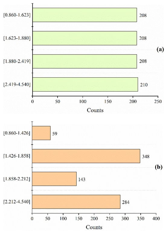
Figure 10. (a) The initial equal-interval division method. (b) The final interval division method by GA.

Figure 11 displays the linear relationships within each I_c interval while simultaneously presenting the direct linear function for the raw data without preprocessing. As indicated by the arrow, the equation $N_{60}=0.097\left(q_t/Pa\right)+8.70$ is represented by a short dash–dot line in Figure 11.

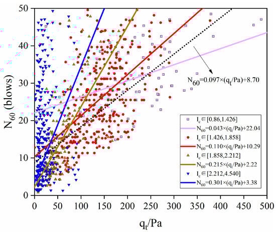
Figure 11. Linear fitting equations across different I_c intervals.

The findings clearly indicate that the data in different intervals exhibit pronounced linear relationships, with RMSE values for the four functions ranging from 7.43 to 8.85. It is noted that all these values are lower than the RMSE of 9.69 obtained from the direct linear function. Although four distinct equations were used for N₆₀ estimation, each data point corresponds to a uniquely predicted value. Figure 12a shows the comparison between all estimated and measured N₆₀ values.

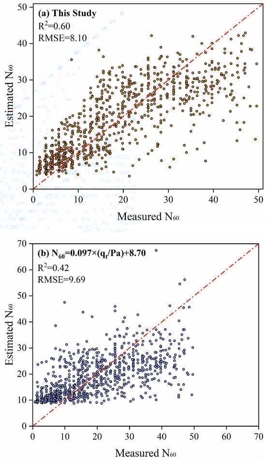
Figure 12. (a) Comparison between estimated and measured N₆₀ values of the proposed segmented model. (b) Comparison between estimated and measured N₆₀ values of the direct linear function.

In contrast, the direct linear function applied to the raw dataset yielded an R² of 0.42 between estimated and measured N₆₀ values, lower than the accuracy achieved by the proposed model. Comparative analyses of Figure 12a,b reveal that the direct linear function was observed to significantly overestimate measured values when N₆₀ < 10, whereas the proposed model eliminated this bias. N₆₀ predictions within the low range (N₆₀ < 10) are predominantly governed by function intercepts rather than linear coefficients; 93% of data in this N₆₀ range are concentrated within the I_c intervals [1.858, 2.212] and [2.212, 4.540]. Within these intervals, the intercepts established for the proposed model are specified as 2.22 and 3.38, respectively. Lower N₆₀ predictions are consistently produced by the proposed model than those generated by the function with an intercept of 8.70 (Figure 12b). This comparison demonstrates that the GA enables more effective extraction of inherent data relationship through I_c interval division, identifying intervals where CPT-q_t and SPT-N₆₀ exhibit similar linear relationships. Consequently, the capability to predict N₆₀ from q_t is substantially enhanced.

5. Comparison and Validation

5.1. Comparison with Artificial Intelligence (AI) Models

Two typical AI algorithms (Random Forest Regression and artificial neural network) are introduced to construct CPT-SPT correlation models. These models are then compared with the proposed model to validate its advantages in simplicity and prediction performance.

Random Forest Regression (RF) is an ensemble learning method that constructs multiple decision trees for prediction and averages their outputs to obtain the final result [38]. Key hyperparameters of the RF model in this study were optimized using Optuna, with the goal of maximizing the R² score during hyperparameter tuning. Bootstrap sampling was also incorporated to enhance variability in the training process. The optimal combination of parameters included a small ensemble of three trees with a maximum depth of 3. The minimum number of samples required to split a node and form a leaf was set to four, while the maximum number of leaf nodes was limited to six. Artificial neural networks (ANNs) are computational models inspired by biological neural networks, consisting of multiple layers of neurons, including an input layer, one or more hidden layers, and an output layer. By adjusting the weights and biases, ANNs are capable of capturing complex nonlinear relationships within data [39]. In this study, a feedforward neural network was developed, consisting of an input layer, two hidden layers, and an output layer. The first hidden layer contains 16 neurons, while the second hidden layer contains 8 neurons. Both hidden layers utilize the ReLU activation function. To mitigate the risk of overfitting, a dropout layer with a rate of 0.01 was incorporated after the first hidden layer. The network weights were updated using the Adam optimizer with an initial learning rate of 0.01. Additionally, the ReduceLROnPlateau learning rate scheduler was employed, with a reduction factor of 0.1 and a patience parameter of 10. The model was trained using a batch size of 32 for a maximum of 1000 epochs. An early stopping mechanism was also implemented to prevent overfitting and ensure efficient training.

In this study, the filtered dataset from the South Island of New Zealand was used to develop prediction models based on RF and an ANN, with q_t, f_s, I_c, and depth as the input features and N₆₀ as the output. During the modeling process, the data across the training and test sets is first ensured to be identical for both methods by fixing the random seed. The performance of both models was validated on the identical testing set and compared with the proposed model, as presented in Figure 13.

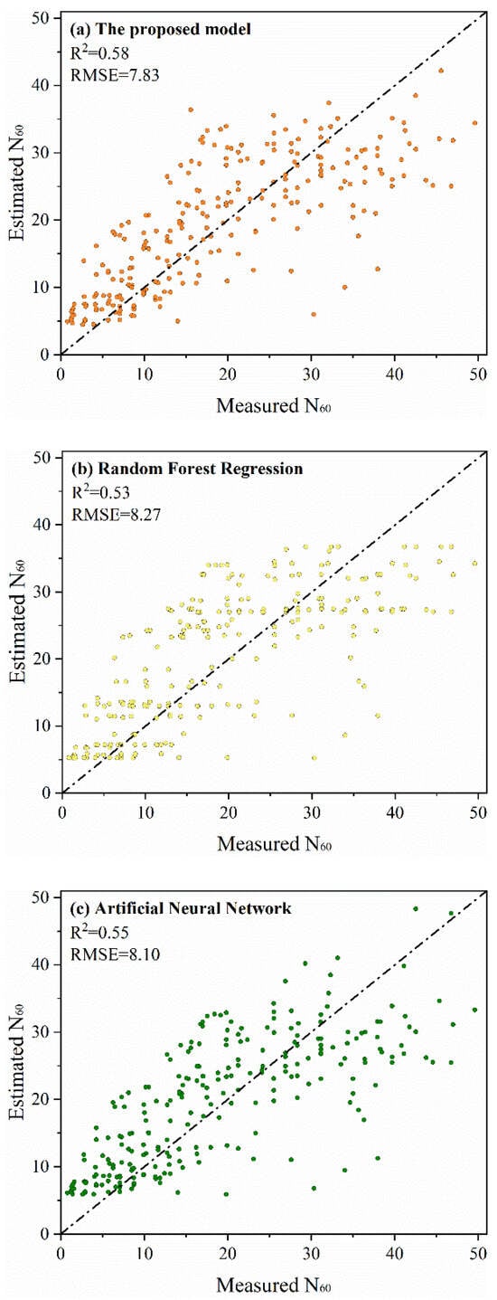
Figure 13. (a) Comparison between estimated and measured N₆₀ values of the proposed model. (b) Comparison between estimated and measured N₆₀ values of the RF model. (c) Comparison between estimated and measured N₆₀ values of the ANN model.

Figure 13 demonstrates the advantages of the proposed model compared with the above two AI-based models; utilizing only two core parameters (q_t and I_c), the proposed model achieves higher predictive accuracy. Specifically, an R² value of 0.58 was attained between estimated and measured N₆₀ values on the testing set of the proposed model, surpassing the RF model with R² = 0.53 and ANN model with R² = 0.55. In this study, the Diebold–Mariano (DM) test was also employed to compare the performance differences among models [40]. Specifically, the predictive accuracy of the proposed model was compared against the ANN and RF models. The results indicate that the DM statistic for the ANN model compared with the proposed model is 2.13, corresponding to a p-value of 0.033; the DM statistic for the RF model compared with the proposed model is 2.83, corresponding to a p-value of 0.005. Since both p-values are less than the conventional significance threshold of 0.05, the differences in prediction errors are statistically significant. This demonstrates that the proposed model developed exhibits significant differences in predictive performance compared to both the ANN and RF models. Moreover, as both DM statistics are positive, this indicates that the error of the ANN and RF exceeds that of the proposed model.

This may be because AI-based models typically possess the ability to uncover complex relationships, but this also means they are more susceptible to fitting random noise. Therefore, they may learn this noise as meaningful patterns, resulting in poor generalization capabilities. The efficient and transparent modeling approach in this study not only simplifies model complexity but also outperforms traditional black-box algorithms in terms of performance, highlighting its potential advantages in both practical applications and theoretical research. These AI models may not be the most advanced solutions, but they serve as key benchmarks to evaluate the practicality of our approach.

5.2. Comparison with Traditional Models

To comprehensively evaluate the performance and applicability of the proposed model, a systematic comparison was conducted with established models from the literature. Since the models developed by Lunne et al. (1997) and Robertson (2012) [21,22] can predict N₆₀ for all soil types and have been widely applied, they were selected for comparison. A comparison between the estimated and measured values for both methods is presented in Figure 14. The Lunne et al. (1997) [21] model yielded an R² of 0.45 and an RMSE of 9.46, while the Robertson (2012) [22] model yielded an R² of 0.37 and an RMSE of 10.11. Both traditional methods exhibit substantially greater dispersion compared to the proposed model, which achieves an R² of 0.60. Additionally, in comparison with the models proposed by Lunne et al. (1997) and Robertson (2012) [21,22], the DM statistics were 6.90 and 7.76, respectively, with corresponding p-values approaching 0 and significantly less than 0.05. These results indicate that the differences in prediction errors between the proposed model and the traditional models are statistically significant.

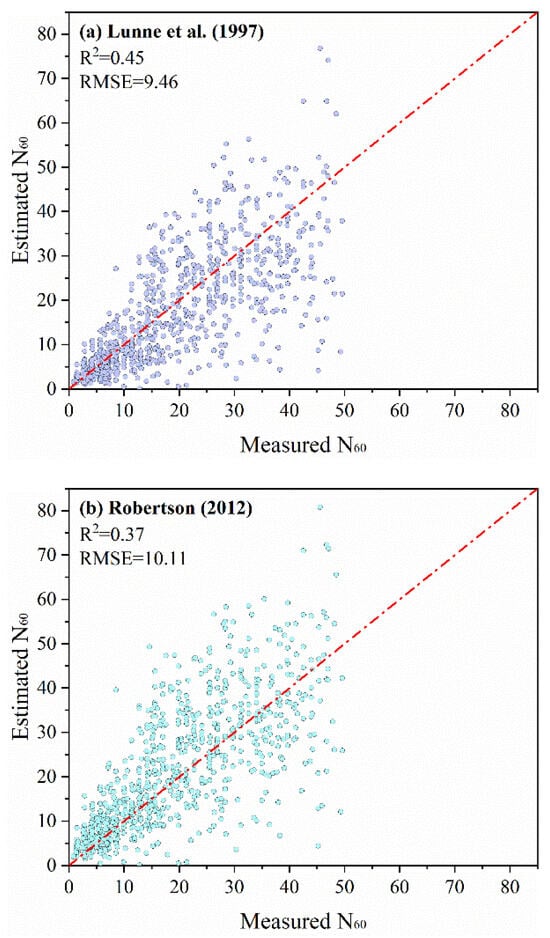
Figure 14. (a) Comparison between estimated and measured N₆₀ values of the Lunne et al. (1997) model [21]. (b) Comparison between estimated and measured N₆₀ values of the Robertson (2012) model [22].

The reasons for the poor performance of these two traditional models may be as follows: The Lunne et al. (1997) model [21] was developed by modifying the Jefferies and Davies (1993) model [19], which established a proportional relationship between q_c/N and I_c. This assumption of proportionality may represent an oversimplification, potentially neglecting nonlinearities between q_c/N and I_c. Lunne et al. (1997) [21] merely refined the coefficient of the Jefferies and Davies (1993) model [19] without making any fundamental changes. Consequently, the Lunne et al. (1997) model [21] may likewise fail to capture the complex interrelationships among N, q_c, and I_c. The Robertson (2012) model [22] also exhibited deviation in prediction of N₆₀. This deficiency may be attributed to its derivation process: the model was formulated through mathematical optimization of existing CPT-SPT correlations without subsequent independent validation.

From the above discussion, it can be concluded that the traditional methods exhibit significantly lower predictive performance on the current dataset compared with the linear models based on I_c interval division proposed in this study. Although the dispersion of the prediction results from the proposed model has not been completely eliminated, a substantial improvement in prediction accuracy has been achieved, indicating that complex relationships within the data have been effectively captured. Under complex geological conditions, the predictive results of the proposed model more closely align with measured values, providing a more reliable basis for future engineering applications.

5.3. Comparison of Different Models on Data from Other Regions

Further analyses are conducted using data from other regions mentioned in Table 3 of Section 4.3, in order to compare the model proposed in this study with other models in new scenarios. Figure 15 presents a comparison of the prediction results from three methods, including the Lunne et al. (1997) model, Robertson (2012) model, and proposed model [21,22].

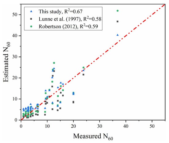
Figure 15. Comparison between estimated and measured N₆₀ values from the models of Lunne et al. (1997), Robertson (2012), and this study [21,22].

It can be observed that the model proposed in this study achieves a higher R² (0.67) compared to other traditional models (0.58 and 0.59), demonstrating its superior predictive accuracy. In conclusion, the proposed model exhibits better agreement between estimated and measured values, providing preliminary validation of its applicability in other regions. However, this model is based on the relationships within a specific regional dataset. It is essential that users conduct thorough evaluation and validation to ensure the reliability and applicability of the model in other regions.

6. Conclusions

The Cone Penetration Test (CPT) and Standard Penetration Test (SPT) are two widely utilized in situ testing methods in geotechnical engineering. Establishing correlations between them is important for engineering applications. This study aims to develop a novel method in this field. In this study, a GA-based simplified linear model between the CPT and SPT was proposed. The dataset was first divided into different I_c intervals using a GA, after which linear regression models between CPT-q_t and SPT-N₆₀ were developed for each interval. Practitioners can use the q_t and I_c data obtained from the CPT to calculate and apply SPT-based design methods through the proposed model. The conclusion of this study is given below:

• The novel Segmented Information Criterion (SIC) is introduced in this study for dual-objective optimization, in which predictive accuracy is balanced against model complexity. The SIC enables quantification of the equilibrium point between these objectives through a unified metric. The weighting coefficients within the SIC were determined by normalizing the South Island of New Zealand dataset, subsequently identifying four I_c intervals as optimal. The introduction of the SIC offers a fresh perspective for future research, enabling a balance between predictive accuracy and model complexity to mitigate the risk of overfitting.
• The powerful search capability of the GA was creatively combined with the simplicity of linear regression to establish a CPT-q_t-and-SPT-N₆₀ relationship. An R² value of 0.58 was achieved by the proposed model on the testing data, representing a 9% and 5% improvement compared with R² values of 0.53 and 0.55 obtained by the RF and ANN methods, respectively. This demonstrates the advantages of the proposed model in both N₆₀ prediction and application. Furthermore, on the dataset from the South Island of New Zealand, the proposed model achieved an R² of 0.60, representing at least a 33% improvement compared to the maximum R² of 0.45 yielded by the commonly used models. This result, combined with its 14% higher predictive accuracy on the dataset in other regions, confirms the higher reliability of the proposed model compared to traditional methods.

In summary, distinct CPT-SPT correlations may be observed under different soil types, and an efficient and practical solution for predicting N₆₀ with complex conditions is provided by the approach proposed in this study, through which a new perspective and methodology are introduced to the research field of CPT-SPT correlation. Compared to conventional black-box AI, the proposed model enhances explainability by being presented solely in the form of a simple linear model. Furthermore, while black-box AI faces operational complexities and practical limitations due to its difficulty in explanation, the proposed model is considered highly operational due to its high explainability. However, the uneven distribution of data across soil types in the development dataset, along with the limited number of validation data points, may limit the generalization capability of the proposed model. And the tuning of SIC parameters may also influence the division outcomes, warranting further investigation. In the future, more data will be collected under various geological conditions to validate the applicability of the proposed model in other regions and further optimize it. Furthermore, exploring the relationship between model parameters and soil properties within this framework will be a focus of future research.

References

- Bolton Seed, H.; Tokimatsu, K.; Harder, L.F.; Chung, R.M. Influence of SPT Procedures in Soil Liquefaction Resistance Evaluations. J. Geotech. Engrg. 1985, 111, 1425–1445. [Google Scholar] [CrossRef]
- Wazoh, H.N.; Mallo, S.J. Standard Penetration Test in Engineering Geological Site Investigations–A Review. Int. J. Eng. Sci. 2014, 3, 40–48. [Google Scholar]
- Akca, N. Correlation of SPT–CPT Data from the United Arab Emirates. Eng. Geol. 2003, 67, 219–231. [Google Scholar] [CrossRef]
- ASTM D5778-07; Standard Test Method for Electronic Friction Cone and Piezocone Penetration Testing of Soils. ASTM International: West Conshohocken, PA, USA, 2020.
- Bol, E. A New Approach to the Correlation of SPT-CPT Depending on the Soil Behavior Type Index. Eng. Geol. 2023, 314, 106996. [Google Scholar] [CrossRef]
- Shahien, M.M.; Albatal, A.H. SPT-CPT Correlations for Nile Delta Silty Sand Deposits in Egypt. In Proceedings of the 3rd International Symposium on Cone Penetration Testing, Las Vegas, NV, USA, 13–14 May 2014; pp. 699–708. [Google Scholar]
- Asef, I.A.; Mohiuddin, A.; Khondaker, S.A. SPT and CPT Correlations for Jolshiri Area of Dhaka Reclaimed by Dredged River Sediments. J. Geoengin. 2023, 18, 225–238. [Google Scholar] [CrossRef]
- Lu, Y.C.; Liu, L.W.; Khoshnevisan, S.; Ku, C.S.; Juang, C.H.; Xiao, S.H. A New Approach to Constructing SPT-CPT Correlation for Sandy Soils. Georisk Assess. Manag. Risk Eng. Syst. Geohazards 2023, 17, 406–422. [Google Scholar] [CrossRef]
- Meyerhof, G.G. Shallow Foundations. J. Soil Mech. Found. Div. 1965, 91, 21–31. [Google Scholar] [CrossRef]
- Schmertmann, J.H. Static Cone to Compute Static Settlement Over Sand. J. Soil Mech. Found. Div. 1970, 96, 1011–1043. [Google Scholar] [CrossRef]
- Danziger, B.; Velloso, D.A. Correlations between the CPT and the SPT for Some Brazilian Soils. Proc. CPT’95 1995, 2, 155–160. [Google Scholar]
- Kara, O.; Gündüz, Z. Correlation between CPT and SPT in Adapazari, Turkey. In Proceedings of the 2nd International Symposium on Cone Penetration Testing, Huntington Beach, CA, USA, 8–12 May 2010. [Google Scholar]
- Zhao, X.; Cai, G. SPT-CPT Correlation and Its Application for Liquefaction Evaluation in China. Mar. Georesources Geotechnol. 2015, 33, 272–281. [Google Scholar] [CrossRef]
- Alam, M.; Aaqib, M.; Sadiq, S.; Mandokhail, S.J.; Adeel, M.B.; Rehman, M.; Kakar, N.A. Empirical SPT-CPT Correlation for Soils from Lahore, Pakistan. IOP Conf. Ser. Mater. Sci. Eng. 2018, 414, 012015. [Google Scholar] [CrossRef]
- Shahri, A.; Juhlin, C.; Malemir, A. A Reliable Correlation of SPT-CPT Data for Southwest of Sweden. Electron. J. Geotech. Eng. 2014, 19, e1032. [Google Scholar]
- Jarushi, F.; AlKaabim, S.; Cosentino, P. A New Correlation between SPT and CPT for Various Soils. Int. J. Geol. Environ. Eng. 2015, 9, 101–107. [Google Scholar]
- Hossain, B.; Zahirul, M.M.; Rahman, A. Correlation Between SPT and CPT of Various Soil Types in Padma River at Mawa (Downstream Side) Near Padma Bridge. In Proceedings of the 7th International Conference on Advances in Civil Engineering, Chittagong University of Engineering and Technology (CUET), Chattogram, Bangladesh, 12–14 December 2024. [Google Scholar]
- Robertson, P.K.; Campanella, R.G.; Wightman, A. SPT-CPT Correlations. J. Geotech. Eng. 1983, 109, 1449–1459. [Google Scholar] [CrossRef]
- Jefferies, M.; Davies, M. Use of CPTu to Estimate Equivalent SPT N60. Geotech. Test. J. 1993, 16, 458–468. [Google Scholar] [CrossRef]
- Robertson, P.K.; Wride, C. (Fear) Evaluating Cyclic Liquefaction Potential Using the Cone Penetration Test. Can. Geotech. J. 1998, 35, 442–459. [Google Scholar] [CrossRef]
- Lunne, T.; Powell, J.J.M.; Robertson, P.K. Cone Penetration Testing in Geotechnical Practice; CRC Press: London, UK, 2014; ISBN 978-0-429-17780-4. [Google Scholar]
- Robertson, P.K. The James K. Mitchell Lecture: Interpretation of in-Situ Tests–Some Insights. In Proceedings of the 4th International Conference on Geotechnical and Geophysical Site Characterization–ISC, Pernambuco, Brazil, 18–21 September 2012; Volume 4, pp. 3–24. [Google Scholar]
- Chin, C.T.; Duann, S.W.; Kao, T.C. SPT-CPT Correlations for Granular Soils. In International Journal of Rock Mechanics and Mining Sciences and Geomechanics Abstracts; Elsevier Science: Amsterdam, The Netherlands, 1990; Volume 27, p. A91. [Google Scholar]
- Kulhawy, F.H.; Mayne, P.W. Manual on Estimating Soil Properties for Foundation Design; Geotechnical Engineering Group; Electric Power Research Inst.: Palo Alto, CA, USA; Cornell University: Ithaca, NY, USA, 1990. [Google Scholar]
- Idriss, I.M.; Boulanger, R.W. Semi-Empirical Procedures for Evaluating Liquefaction Potential during Earthquakes. Soil Dyn. Earthq. Eng. 2006, 26, 115–130. [Google Scholar] [CrossRef]
- Arifuzzaman; Anisuzzaman, M. An Initiative to Correlate the SPT and CPT Data for an Alluvial Deposit of Dhaka City. Int. J. Geo-Eng. 2022, 13, 5. [Google Scholar] [CrossRef]
- Cheng, X.; Liu, X.; Qiao, H.; Wu, Z.; Cai, G. A New SPT-CPT Correlation by Statistical Analysis Based on a Database from Anhui, China. Georisk Assess. Manag. Risk Eng. Syst. Geohazards 2024, 18, 838–853. [Google Scholar] [CrossRef]
- Tarawneh, B. Predicting Standard Penetration Test N-Value from Cone Penetration Test Data Using Artificial Neural Networks. Geosci. Front. 2017, 8, 199–204. [Google Scholar] [CrossRef]
- Al Bodour, W.; Tarawneh, B.; Murad, Y. A Model to Predict the Standard Penetration Test N60 Value from Cone Penetration Test Data. Soil Mech. Found. Eng. 2022, 59, 437–444. [Google Scholar] [CrossRef]
- Bai, R.; Shen, F.; Zhao, Z.; Zhang, Z.; Yu, Q. The Analysis of the Correlation between SPT and CPT Based on CNN-GA and Liquefaction Discrimination Research. CMES 2024, 138, 1159–1182. [Google Scholar] [CrossRef]
- Ansary, M.A.; Ansary, M. Use of CPT and Other Parameters for Estimating SPT-N Value Using Optimised Machine Learning Models. J. Geoengin. 2024, 19, 83–94. [Google Scholar] [CrossRef]
- Zhou, H.; Wotherspoon, L.M.; Hayden, C.P.; McGann, C.R.; Stolte, A.; Haycock, I. Assessment of Existing SPT–CPT Correlations Using a New Zealand Database. J. Geotech. Geoenviron. Eng. 2021, 147, 04021131. [Google Scholar] [CrossRef]
- Robertson, P.K. Guide to Cone Penetration Testing for Geotechnical Engineering. Available online: https://www.scribd.com/document/510873365/6th-Edition-of-Guide-to-Cone-Penetration-Testing-now-available-Gregg-Drilling-LLC (accessed on 24 December 2025).
- Williamson, D.F.; Parker, R.A.; Kendrick, J.S. The Box Plot: A Simple Visual Method to Interpret Data. Ann. Intern. Med. 1989, 110, 916–921. [Google Scholar] [CrossRef] [PubMed]
- Schober, P.; Boer, C.; Schwarte, L.A. Correlation Coefficients: Appropriate Use and Interpretation. Anesth. Analg. 2018, 126, 1763–1768. [Google Scholar] [CrossRef]
- Lambora, A.; Gupta, K.; Chopra, K. Genetic Algorithm-A Literature Review. In Proceedings of the 2019 International Conference on Machine Learning, Big Data, Cloud and Parallel Computing (COMITCon), Faridabad, India, 14–16 February 2019; IEEE: New York, NY, USA, 2019; pp. 380–384. [Google Scholar]
- Han, X.; Gong, W.; Juang, C.H.; Bowa, V.M.; Khoshnevisan, S. CPTu-SPT Correlation Analyses Based on Pairwise Data in Southwestern Taiwan. Georisk Assess. Manag. Risk Eng. Syst. Geohazards 2022, 16, 622–639. [Google Scholar] [CrossRef]
- Breiman, L. Random Forests. Mach. Learn. 2001, 45, 5–32. [Google Scholar] [CrossRef]
- Zupan, J. Introduction to Artificial Neural Network (ANN) Methods: What They Are and How to Use Them. Acta Chim. Slov. 1994, 41, 327. [Google Scholar]
- Chen, H.; Wan, Q.; Wang, Y. Refined Diebold-Mariano Test Methods for the Evaluation of Wind Power Forecasting Models. Energies 2014, 7, 4185–4198. [Google Scholar] [CrossRef]
Disclaimer/Publisher’s Note: The statements, opinions and data contained in all publications are solely those of the individual author(s) and contributor(s) and not of MDPI and/or the editor(s). MDPI and/or the editor(s) disclaim responsibility for any injury to people or property resulting from any ideas, methods, instructions or products referred to in the content. |
© 2025 by the authors. Licensee MDPI, Basel, Switzerland. This article is an open access article distributed under the terms and conditions of the Creative Commons Attribution (CC BY) license.