Snow Depth Estimation with Combined Terrain and Remote Sensing Information over High-Latitude Asia

Abstract

High-resolution snow depth monitoring is a crucial foundation for precise disaster early warning and optimal water resource management. Traditional snow depth estimation methods mainly rely on passive microwave remote sensing data, but due to their low spatial resolution, they have difficulties capturing the subtle changes in snow depth in complex terrain. Existing deep learning methods mostly adopt single-modal or simple band fusion, failing to fully utilize the complementarity among multi-source data and not considering that terrain factors can lead to misjudgment of the true snow signal. Therefore, this paper proposes a dual-branch intermediate fusion network (TACMF-Net) for high-latitude regions in Asia. By introducing terrain factors (DEM, slope, aspect) and conducting cross-modal feature interaction, it achieves efficient collaboration of multi-source remote sensing data. Research shows that our method has extremely high accuracy and robustness on the self-made multi-source snow depth terrain dataset.

1. Introduction

As one of the most common seasonal land cover types on the Earth’s surface, snow cover is widely distributed in mid-to-high latitudes and high-altitude regions, serving as a crucial variable in the global climate system and hydrological cycle [1,2]. The spatiotemporal distribution of snow has a profound impact on the regional climate regulation, ecosystem evolution, and carbon cycle [3,4]. Particularly in the high-latitude mountainous environments of Asia, such as the Tibetan Plateau, Altai Mountains, Tianshan Mountains, and the Himalayas, snowpack not only acts as a vital water resource reservoir but is also a key trigger for disasters like avalanches, landslides, and floods [5,6,7]. Moreover, snowpack stores a large volume of winter precipitation, which directly influences watershed hydrological processes during the spring melt, agricultural irrigation scheduling, and cross-seasonal water security [8,9]. Snow depth, as the most direct indicator of snow volume, thickness, and spatial distribution, is a critical parameter for perceiving snow status and predicting its evolutionary trends [10]. Consequently, research on high-precision, wide-coverage snow depth estimation has become a core interdisciplinary topic at the intersection of remote sensing, geographic information science, hydrology, and disaster prevention.

Traditional snow depth observation has primarily relied on ground-based meteorological stations, manual measurements, and snow ruler readings. Despite their high accuracy, these methods are hampered by high labor costs, sparse station distribution, and limited spatial coverage due to complex terrain and harsh weather conditions, posing significant challenges in high-altitude cold regions and uninhabited areas [11]. With the advancement of remote sensing technology, an increasing variety of high-resolution, multi-source remote sensing data—including optical, passive microwave, Synthetic Aperture Radar (SAR), and LiDAR—has been applied to snow retrieval. This has provided substantial informational support and technical assurance for monitoring snow’s spatial distribution, depth changes, and dynamics, enhancing the detection capabilities in complex terrain and remote cold regions [12,13,14,15]. Passive microwave remote sensing (e.g., AMSR-E) models the brightness temperature (BT) difference between snow and the ground surface to retrieve snow depth, offering all-weather capabilities and wide coverage. For instance, the Killy algorithm utilizes passive microwave scattering signals from spaceborne instruments to detect snowpack [16]. Active radar remote sensing, such as SAR, inverts snow depth through the propagation delay of radar waves and leverages SAR’s coherence and phase information to extract snow characteristics. It has high spatial resolution and can penetrate clouds. For example, Leinss et al. analyzed the anisotropic features of seasonal snow using polarimetric SAR phase differences, proposing a retrieval method based on polarimetric phase difference that offers new insights for snow depth estimation [17]. LiDAR, using airborne or satellite-based lasers (e.g., ICESat), determines the surface elevation difference before and after snowfall and is suitable for snow estimation in forests and mountains. Due to its high sensitivity to surface deformation and snow depth changes, LiDAR is progressively becoming a key tool in snow monitoring research [18]. Additionally, optical remote sensing acquires snow cover information via optical sensors and indirectly estimates snow depth by combining it with temperature and precipitation data. It is characterized by high spatial resolution. For instance, Parajka et al. improved snow cover information extraction through spatiotemporal fusion of MODIS imagery, providing an effective means for large-scale, high-frequency snow cover monitoring [19].

In addition to remote sensing retrieval, another traditional approach to snow depth estimation is numerical simulation. These methods are typically based on the principles of energy and mass conservation, integrating meteorological variables (e.g., temperature, precipitation, wind speed) and land surface attributes (e.g., soil, vegetation) to dynamically simulate the formation, evolution, and melting of snowpack. Such models are founded on robust physical mechanisms and can provide continuous outputs of snow depth or snow water equivalent in both time and space. The Crocus model, developed by Vionnet et al., can finely simulate snowpack thermal and moisture fluxes and is a primary tool for snow depth simulation in European mountainous regions [20]. The Noah-MP model, embedded in meteorological-hydrological coupled systems, is suitable for long-term snow process simulation at regional or global scales [21]. Although numerical simulations do not directly rely on image information, they are increasingly being coupled with remote sensing data to better investigate snow depth patterns. For example, Kumar et al. assimilated snow depth products from AMSR-E and MODIS into the Noah-MP model, which improved the spatial consistency of simulations and their accuracy in mountainous areas [22]. Xue et al. assimilated passive microwave brightness temperature observations from AMSR-E into NASA’s Catchment land surface model, using a Support Vector Machine (SVM) as the observation operator combined with a 1D Ensemble Kalman Filter (1D-EnKF) to estimate snow mass over North America [23].

However, numerical simulation methods for snow depth face certain challenges: their model structures are complex, they involve numerous parameters, and they are computationally expensive with long run times, which limits their widespread use in large-scale, real-time applications. Benefiting from advancements in artificial intelligence and hardware, a growing number of scholars are turning to data-driven approaches, employing machine learning and deep learning for end-to-end snow depth estimation. Hu et al. used various machine learning methods to fuse remote sensing data and ground observations, creating a high-precision snow depth product for the Northern Hemisphere that improved spatial resolution [24]. Yao et al. proposed a novel retrieval method based on a deep convolutional neural network (ConvNet) to extract snowpack thickness and temperature from passive microwave data, demonstrating higher accuracy and stronger noise resistance than traditional retrieval methods [25]. Although remote sensing data play a crucial role in snow depth estimation, especially in high-altitude cold regions where ground observations are scarce, a single remote sensing source often has limitations. For instance, optical remote sensing is susceptible to cloud cover, while SAR radar data can be noisy and require complex post-processing. Consequently, the development of snow depth estimation models based on multi-source remote sensing data is of great significance [26,27,28,29]. Daudt et al. proposed a model combining convolutional and recurrent neural networks to achieve weekly updated, 10-m spatial resolution snow depth estimates at a national scale from multi-source remote sensing data, without requiring ground station data [30]. Many other researchers have also proposed excellent deep learning models for snow depth estimation. For example, Xing et al. applied a deep residual network to snow depth estimation and were the first to propose a region-to-point estimation method, which significantly improved the spatial resolution and accuracy of snow depth estimates on the Tibetan Plateau [13]. Zhao et al. fused multispectral optical satellite images, SAR images, and land cover maps to create an 8-channel snow dataset, further enhancing the accuracy of snow depth estimation [28].

Nevertheless, most existing deep learning methods for snow depth estimation generally overlook the influence of terrain factors in their model architecture, failing to effectively incorporate key topographic variables such as elevation, slope, and aspect. In high-latitude mountainous areas, topographic conditions significantly regulate the spatial distribution and stability of snowpack. Specifically, higher elevations correspond to lower temperatures, making it easier for snow to form and persist. Areas with gentle slopes are more conducive to snow accumulation, whereas steep slopes often lead to snow sliding or avalanches. Aspect influences the intensity of solar radiation received by the surface; south-facing slopes (in the Northern Hemisphere) are typically warmer with faster snowmelt, while north-facing slopes are cooler and retain snow longer. Without considering these topographic constraints, models cannot accurately capture the spatial variations in snow depth in complex terrain, leading to systematic biases and estimation distortions.

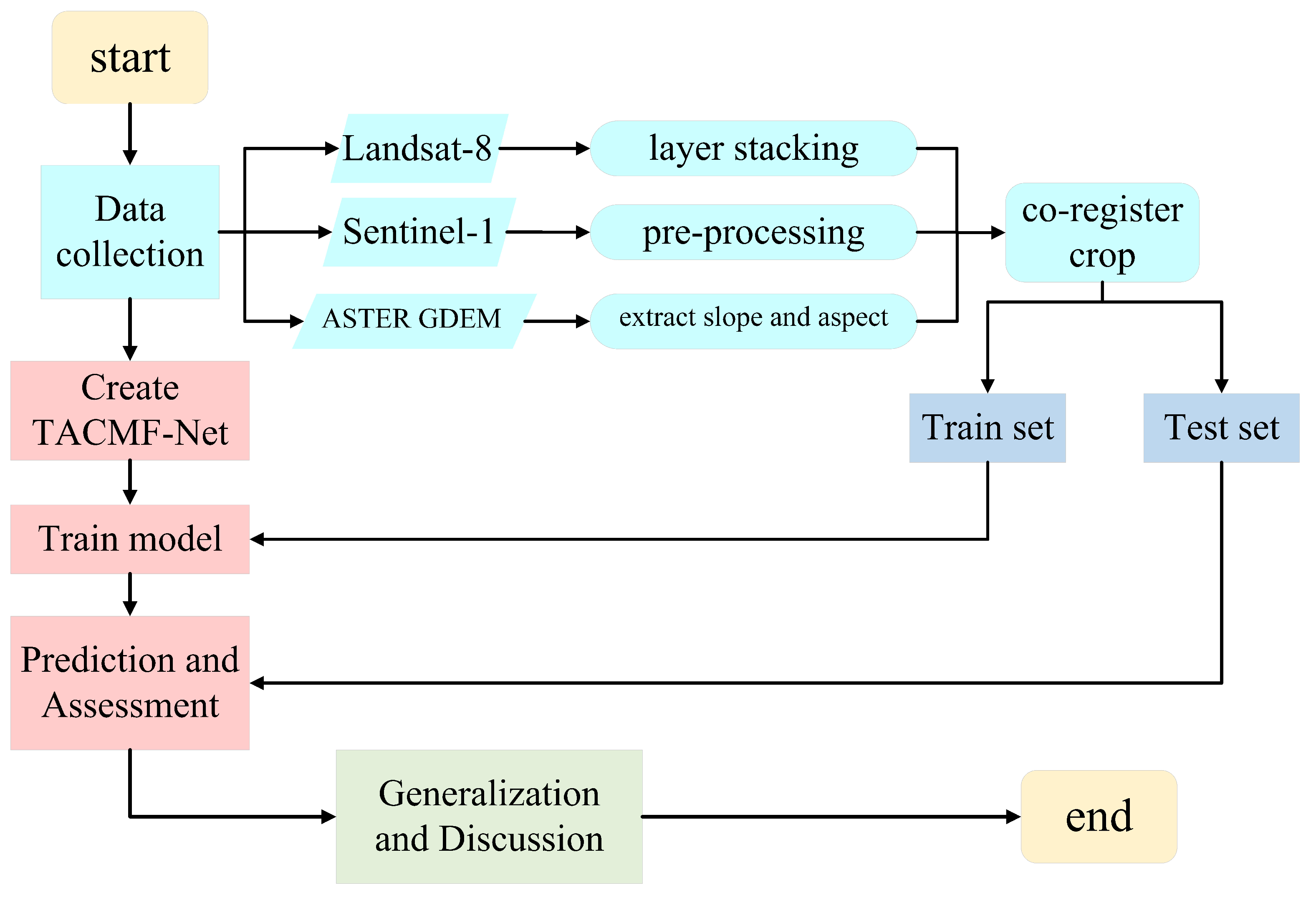
Existing snow depth estimation methods have limitations when applied to high latitudes in Asia, primarily concerning the neglect of complex topographic features and inadequate modeling of spatial heterogeneity in mountainous snowpack. Furthermore, although multi-source remote sensing data (such as active microwave and optical) are widely used, the interaction mechanisms between different modalities in existing models are often not fully exploited, which limits the depth and accuracy of the fused information. We conduct our research to address these issues. Our complete workflow is shown in Figure 1.

Figure 1. Overall flowchart of our work.

Our contributions are as follows:

• A multi-modal fusion snow depth estimation method for parts of high latitudes in Asia is proposed. By introducing a terrain-aware mechanism and a modality interaction module, our method effectively enhances the model’s ability to understand the relationship between topography and remote sensing modality features, thereby improving estimation accuracy and generalization in mountainous snow environments.
• We perform large-scale, high-resolution snow depth mapping at the 100-km scale using our model, enabling the observation of any region of interest and the monitoring of regional snow cover changes.
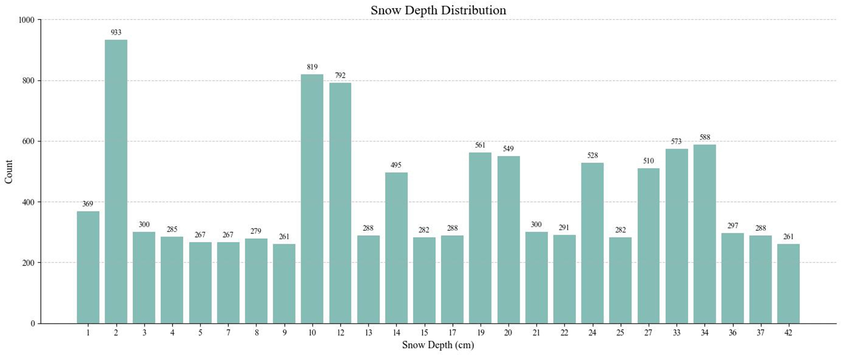
• By incorporating DEM and its derivatives (slope and aspect), we have constructed a multi-source snow depth terrain dataset for the high-latitude regions of Asia, providing data support for future research.

2. Datasets

2.1. Study Area

This study selects typical high-cold regions in western China as the research area, as shown in Figure 2, covering the Qinghai-Tibet Plateau, the Tianshan Mountains in Xinjiang, and the Qilian Mountains in Gansu. Specifically, our research and data collection focus on the high-altitude areas of these high-cold regions, mostly within the orange areas in Figure 2 (the blue areas correspond to low-altitude regions), with the red triangles representing ground snow measurement stations. The region features diverse landforms, including a complex terrain pattern of intertwined plateaus and mountains, with locally steep slopes and variable aspects. Winters are extremely cold, with precipitation primarily in the form of snow, leading to widespread seasonal snow cover [31]. Constrained by terrain obstruction and climatic conditions, conventional snow depth monitoring methods have insufficient coverage in this region. Simultaneously, remote sensing retrieval is susceptible to interference from topographic shadows and the complexity of the snowpack structure, which reduces accuracy. Therefore, this region provides significant experimental value for testing the model’s robustness and generalization capability under complex terrain and variable environmental conditions.

Figure 2. The figure uses distinct colors to differentiate elevation levels. The red triangles represent ground snow stations, all located in high-altitude areas, representing our study area.

2.2. Optical Imagery Data

The optical imagery data for this study were acquired from the Landsat-8 satellite via the official USGS EarthExplorer platform https://earthexplorer.usgs.gov/ (accessed on 1 June 2024). The time period selected was the 175 winter season from 2014 to 2017. To ensure image quality and subsequent co-registration with radar imagery, only images with minimal cloud cover and good visibility on the acquisition day were selected. We utilized the red, green, blue, and near-infrared (NIR) bands. Using the ENVI 5.3 software, we stacked these four bands into a multi-spectral composite and resampled them from 30 m to a 10-m resolution for spatial consistency with the SAR imagery.The resulting four-channel multispectral images provided a crucial optical perspective for the subsequent analysis.

2.3. SAR Imagery Data

The SAR data utilized were C-band data from Sentinel-1, featuring a 10-m spatial resolution. We selected the VV-polarized Ground Range Detected (GRD) products, acquired from the Copernicus Data Space Ecosystem https://dataspace.copernicus.eu/ (accessed on 1 June 2024).Take the same time corresponding to the optical image. We used the SNAP 8.0 toolbox to perform standardized processing on the raw imagery, including orbit correction, noise removal, radiometric calibration, and terrain correction. The final images were converted into intensity images in decibels (dB). As radar imaging is unaffected by cloud cover, precipitation, or illumination changes, these data provide more stable information for snow depth analysis.

2.4. DEM Elevation Data

To incorporate topographic information, this study utilized the ASTER Global Digital Elevation Model (GDEM) with a 30 m spatial resolution, sourced from the China Geoscience Data Cloud https://www.gscloud.cn/ (accessed on 1 June 2024). The time period selected was the winter season from 2014 to 2017. Within the ENVI software environment, we extracted slope and aspect from the raw elevation data and combined them with the original DEM raster to construct a three-channel terrain information image. Subsequently, this image was resampled to a 10 m spatial resolution to achieve resolution consistency with the optical and radar imagery.

2.5. Ground Station Data

To support model training and evaluation, we incorporated in-situ snow depth measurements from the National Meteorological Information Center http://data.cma.cn/ (accessed on 16 May 2020). We selected data from multiple meteorological observation stations covering the study area during the winter periods (primarily November to March) from 2014 to 2017. The observation frequency is once a day. The observation data included station ID, latitude and longitude coordinates, and the measured snow depth for the corresponding dates. The snow depth values ranged from 0 to 42 cm, covering various conditions from snow-free ground to deep snowpack.

2.6. Dataset Construction Pipeline

Currently, high-resolution remote sensing datasets suitable for snow depth retrieval in the high-altitude regions of Asia are still scarce, particularly those integrating radar and topographic information. To this end, we constructed a multi-source terrain-remote sensing snow depth dataset. It encompasses optical remote sensing (Landsat-8), radar remote sensing (Sentinel-1), and digital elevation data (ASTER GDEM) along with its derivatives, all labeled with ground station observations as ground truth for snow depth. All remote sensing images were co-registered and cropped through a unified pre-processing pipeline.

Specifically, we first selected cloud-free optical images and corresponding SAR data based on the meteorological station observation times. After completing image processing and co-registration using ENVI and SNAP tools, we incorporated the 30 m ASTER GDEM data to enhance the model’s understanding of topographic variations. We extracted slope and aspect to create a three-channel terrain feature image, which was also resampled to 10 m and co-registered. Finally, we extracted image patches of 32 × 32 pixels for high-resolution snow depth estimation. The final dataset contains 10,953 samples. For subsequent comparative experiments, we also processed each sample group into an 8-channel input.

Optical images in the visible and near-infrared bands are mainly used to ’see’ where the snow is and to initially assess the snow surface conditions; SAR radar images can penetrate shallow snow layers and detect the internal structure of the snow; elevation and terrain factors determine where snow is most likely to accumulate and persist. These three provide information based on different physical principles (reflection, scattering, terrain constraints), each with its own role, non-overlapping, and together enhance the accuracy of the model.

Figure 3 shows examples of the combined data sources, and Figure 4 presents the numerical distribution of the snow depth labels.

Figure 3. Examples of the multi-source data inputs for two different samples in the dataset.

Figure 4. The numerical distribution of snow depth labels (in cm) from the ground station data.

3. Methodology

In this study, snow depth estimation is modeled as a remote sensing regression problem. Confronted with challenges such as significant modality differences in multi-source remote sensing imagery and irregular terrain, traditional convolutional neural network architectures often struggle to balance comprehensive information representation with spatial context modeling. To address this, we propose the Terrain-Aware Cross-Modality Fusion Network (TACMF-Net), which aims to fully integrate remote sensing imagery while embedding topographic information. This network constructs a deep semantic interaction mechanism across modalities, leveraging the complementary characteristics of multi-source data and the regulatory role of terrain on snow distribution to enhance the accuracy and generalization capability of regional-scale snow depth estimation. While the model is broadly adaptable to snow depth estimation in various regions, it exhibits stronger feature perception and modeling capabilities, particularly in mountainous environments with drastic terrain variations and significant spatial heterogeneity. The core idea is to use terrain factors to guide the modality feature extraction process, thereby improving the accuracy of regional snow depth estimation.

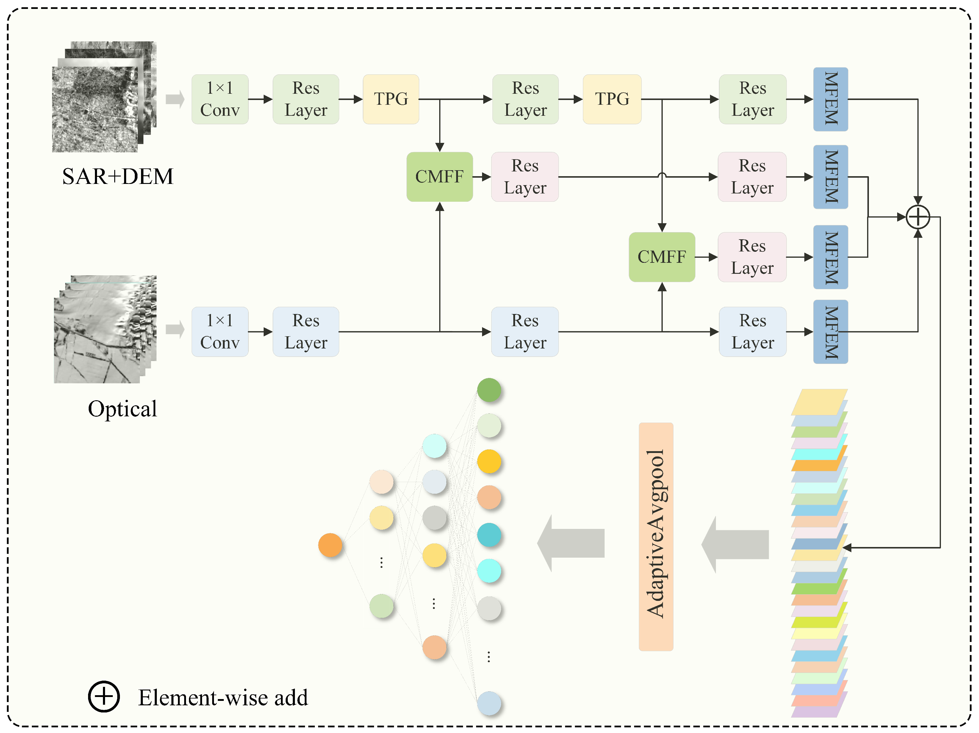
As depicted in Figure 5, TACMF-Net is primarily composed of several key modules: a two-branch residual feature extraction network (Optical Branch and SAR Branch), a Terrain-Aware Guidance (TPG) module, a Cross-Modality Feature Fusion (CMFF) module, and a Multi-scale Feature Perception (MFPM) module.

Figure 5. The overall architecture of the Terrain-Aware Cross-Modality Fusion Network (TACMF-Net), illustrating the main modules and data flow.

3.1. Two-Branch Residual Backbone

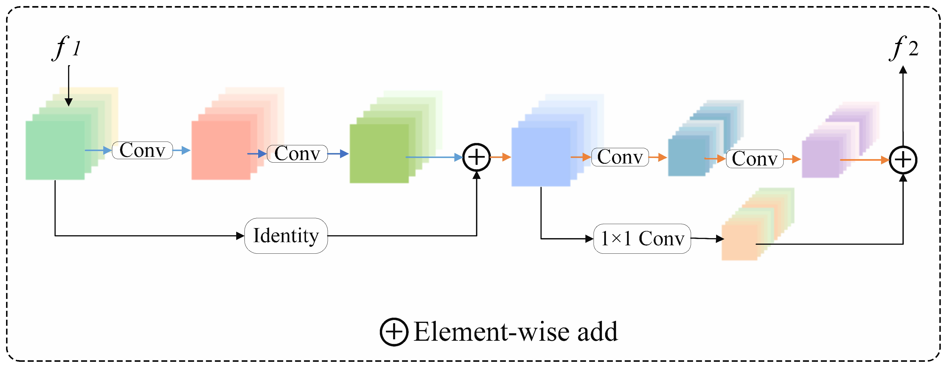
To more accurately estimate snow depth, we designed a two-branch residual network structure, as shown in Figure 6. Since optical and SAR data possess distinct physical properties, direct fusion could lead to information confounding. To fully extract snow-related semantic features from multi-source data, we constructed separate Optical and SAR branches, adopting a ResNet-style residual structure as the fundamental backbone. Its residual modules, through skip connections, pass input features directly to the output layer, which alleviates the training difficulty of deep networks and effectively prevents the problems of vanishing and exploding gradients [32]. Each level of the residual layers contains two residual blocks. The formula for a residual block is expressed as follows:

$${\mathbf{x}}_{i+1}={\mathbf{x}}_i+{\mathrm{Conv}}_{i+1}\left(\mathrm{ReLU}\left({\mathrm{Conv}}_i\left({\mathbf{x}}_i\right)\right)\right).$$

(1)

Figure 6. The two-branch residual backbone structure for feature extraction from optical and SAR data.

This design not only preserves the characteristics of each data type but also enables feature complementarity and enhancement in the subsequent fusion modules. The Optical Branch receives 4-channel optical images, and the SAR Branch receives 4-channel radar images. Upon entering the network, both the optical and SAR images first pass through a 1 × 1 convolution to increase the number of channels. They then undergo three levels of residual extraction modules, with channel dimensions of 32, 64, and 128, corresponding to low-level, mid-level, and high-level semantic representations, respectively. Each residual layer contains two BasicBlock units. The Optical Branch progressively extracts multispectral features through a downsampling sequence, while the SAR Branch employs a symmetric downsampling strategy and embeds the Terrain-Aware Guidance (TPG) module after the first and second residual layers to form a dual spatial-channel visual representation. The two-branch design, through differentiated receptive field expansion strategies, allows the Optical Branch to focus on land cover features and the SAR Branch to strengthen terrain structure information.

3.2. Terrain-Aware Guidance (TPG) Module

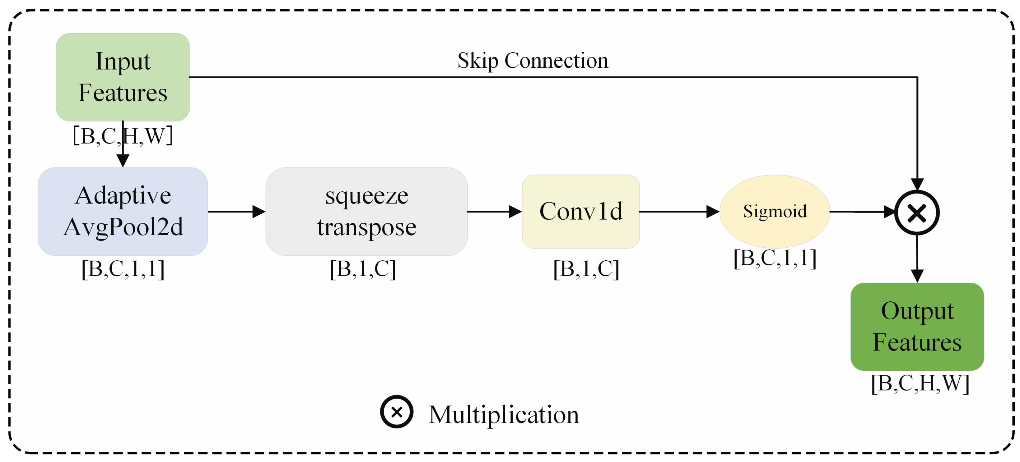
In remote sensing imagery, topographic factors such as elevation, slope, and aspect significantly influence the formation and distribution of snow. To enhance the model’s perception of this topographic information, we introduce the Terrain-Aware Guidance (TPG) module into the SAR branch as a lightweight yet efficient mechanism for terrain awareness, as shown in Figure 7. This module utilizes a channel attention mechanism to adaptively adjust the importance of different channel features, thereby strengthening the model’s responsiveness to topographically dominant regions.

Figure 7. The architecture of the Terrain-Aware Guidance (TPG) module.

Structurally, the TPG module first performs adaptive average pooling on the input feature map across the spatial dimensions to extract channel-level global statistical features. It then captures local dependencies among adjacent channels through a transpose operation and a 1D convolution. Subsequently, the channel weights are normalized using a Sigmoid activation function. Finally, the resulting weight vector is multiplied element-wise with the input feature map to produce an enhanced feature map of the same size as the input. This module is computationally simple and efficient, yet it effectively improves the model’s ability to discriminate terrain-sensitive areas, making it particularly suitable for snow depth estimation tasks in regions with complex and rugged terrain. The core idea is to achieve dynamic recalibration of features along the channel dimension while preserving spatial structure, enabling the model to focus more on semantic information that is closely related to topographic features.

3.3. Cross-Modality Feature Fusion (CMFF) Module

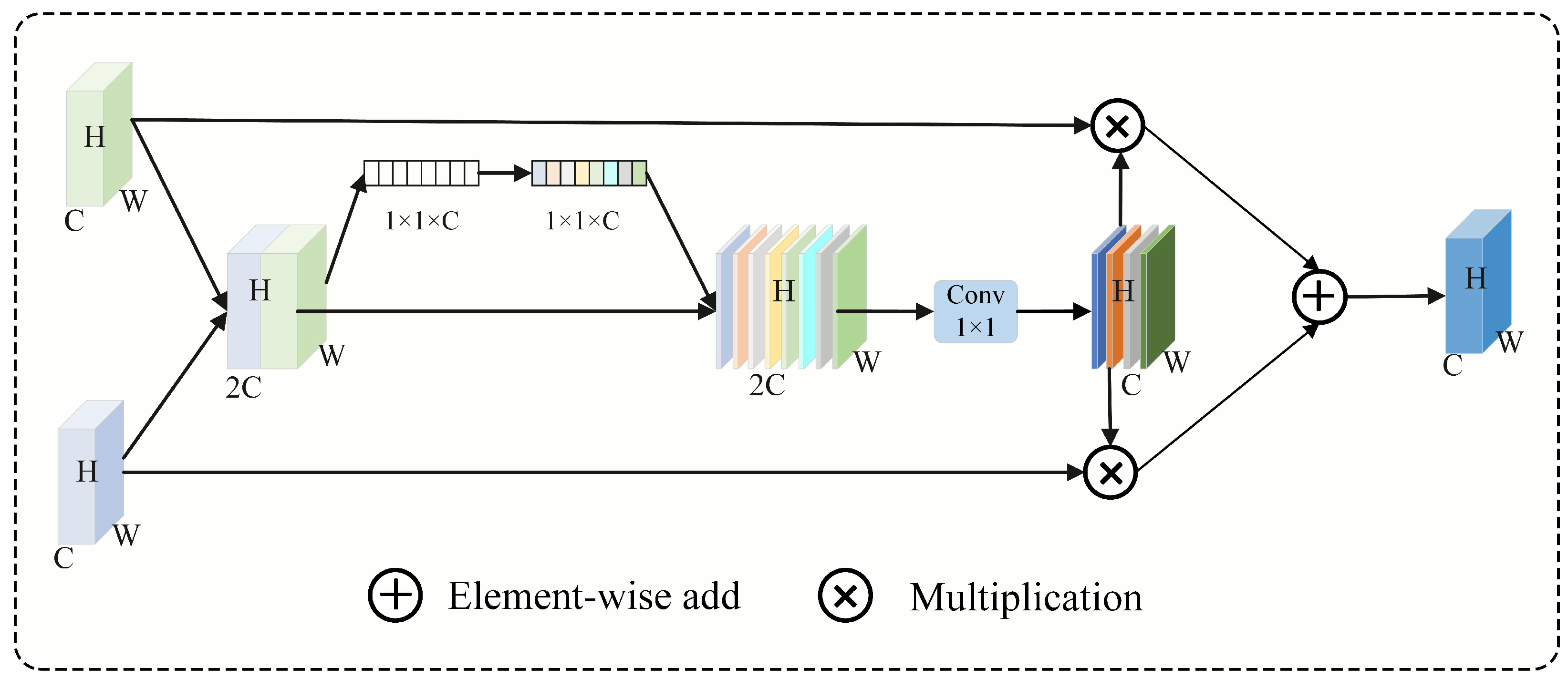
Optical and SAR images provide information from different perspectives: optical images offer stronger spectral and textural representations of the surface, while SAR images have the advantage of penetrating clouds and reflecting topographic variations. However, the feature disparities between these modalities also pose a fusion challenge—simply concatenating features from both modalities can introduce redundancy, potentially weakening key feature expressions and causing learning biases. Considering that the features extracted by the Optical and SAR branches are semantically complementary, we introduce the Cross-Modality Feature Fusion (CMFF) module to enhance the model’s collaborative modeling capabilities across different modalities, as shown in Figure 8. The CMFF module structurally borrows from the channel attention mechanism of SENet, proposed by Hu et al. (2018) [33], and combines it with a guided fusion strategy for optical-SAR feature pairs, ultimately achieving a deep fusion process characterized by mutual guidance, mutual enhancement, and structural alignment. As shown in its structural diagram, the core steps are as follows:

Figure 8. The architecture of the Cross-Modality Feature Fusion (CMFF) module.

First, features are concatenated to generate guided attention weights. Let the feature maps extracted from the optical and SAR images by their respective branches be ${\mathbf{f}}_{\mathrm{opt}},{\mathbf{f}}_{\mathrm{sar}}\in {\mathbb{R}}^{C\times H\times W}$, $\mathbf{C},\mathbf{H},\mathbf{W}$ represent the number of input channels, height, and width, respectively. A concatenated input feature is obtained through a channel-wise concatenation operation:

$${\mathbf{f}}_{\mathrm{cat}}=\mathrm{Concat}({\mathbf{f}}_{\mathrm{opt}},{\mathbf{f}}_{\mathrm{sar}})\in {\mathbb{R}}^{2C\times H\times W}.$$

(2)

Subsequently, to capture channel dependencies, the CMFF module employs a global average pooling operation to squeeze the concatenated feature map, yielding a global channel descriptor vector:

$${\mathbf{f}}_{\mathrm{sq}}={\displaystyle \frac{1}{H\times W}}\sum _{i=1}^H\sum _{j=1}^W{\mathbf{f}}_{\mathrm{cat}}(i,j)\in {\mathbb{R}}^{2C}.$$

(3)

Next, this channel descriptor vector passes through two fully connected (FC) layers, with a ReLU activation function for non-linear mapping in between. $\delta$ represents the activation function, and ${\mathbf{W}}_1$${\mathbf{W}}_2$ are the output features of the two fully connected layers. Finally, a Sigmoid function outputs the channel attention weights:

$${\mathbf{f}}_{\mathrm{ex}}=\sigma ({\mathbf{W}}_2·\delta ({\mathbf{W}}_1·{\mathbf{f}}_{\mathrm{sq}}))\in {\mathbb{R}}^{2C}.$$

(4)

After obtaining the attention weights, they are applied channel-wise to the original concatenated feature map to produce a weighted feature map:

$${\mathbf{f}}_{\mathrm{att}}={\mathbf{f}}_{\mathrm{ex}}\otimes {\mathbf{f}}_{\mathrm{cat}}.$$

(5)

Then, to compress the channel dimension, the CMFF uses a combination of a 1 × 1 convolution, BatchNorm, and ReLU to obtain a structurally aligned and informationally condensed fused feature map:

$${\mathbf{f}}_{\mathrm{refined}}=\mathrm{ReLU}\left(\mathrm{BN}\left({\mathrm{Conv}}_{1\times 1}\left({\mathbf{f}}_{\mathrm{att}}\right)\right)\right)\in {\mathbb{R}}^{C\times H\times W}.$$

(6)

To restore the divisibility between the modalities, the module uses the fused feature map to guide the modulation of the original features from each modality:

$$\begin{array}{cc}\hfill {\mathbf{f}}_{\mathrm{opt}}^{\prime }& ={\mathbf{f}}_{\mathrm{refined}}\otimes {\mathbf{f}}_{\mathrm{opt}},\hfill \end{array}$$

(7)

$$\begin{array}{cc}\hfill {\mathbf{f}}_{\mathrm{sar}}^{\prime }& ={\mathbf{f}}_{\mathrm{refined}}\otimes {\mathbf{f}}_{\mathrm{sar}}.\hfill \end{array}$$

(8)

Finally, the two weighted modality features are added channel-wise to produce the final cross-modality fused output:

$${\mathbf{f}}_{\mathrm{fused}}={\mathbf{f}}_{\mathrm{opt}}^{\prime }\oplus {\mathbf{f}}_{\mathrm{sar}}^{\prime }.$$

(9)

To enhance the model’s cross-modal perception at different feature levels, the CMFF module is deployed between the mid-level (64 channels) and high-level (128 channels) features of the branches. This facilitates multi-level, multi-scale joint modeling of optical and SAR features, significantly improving the model’s adaptability to spatial structures and its semantic alignment capabilities.

3.4. Multi-Scale Feature Perception (MFPM) Module

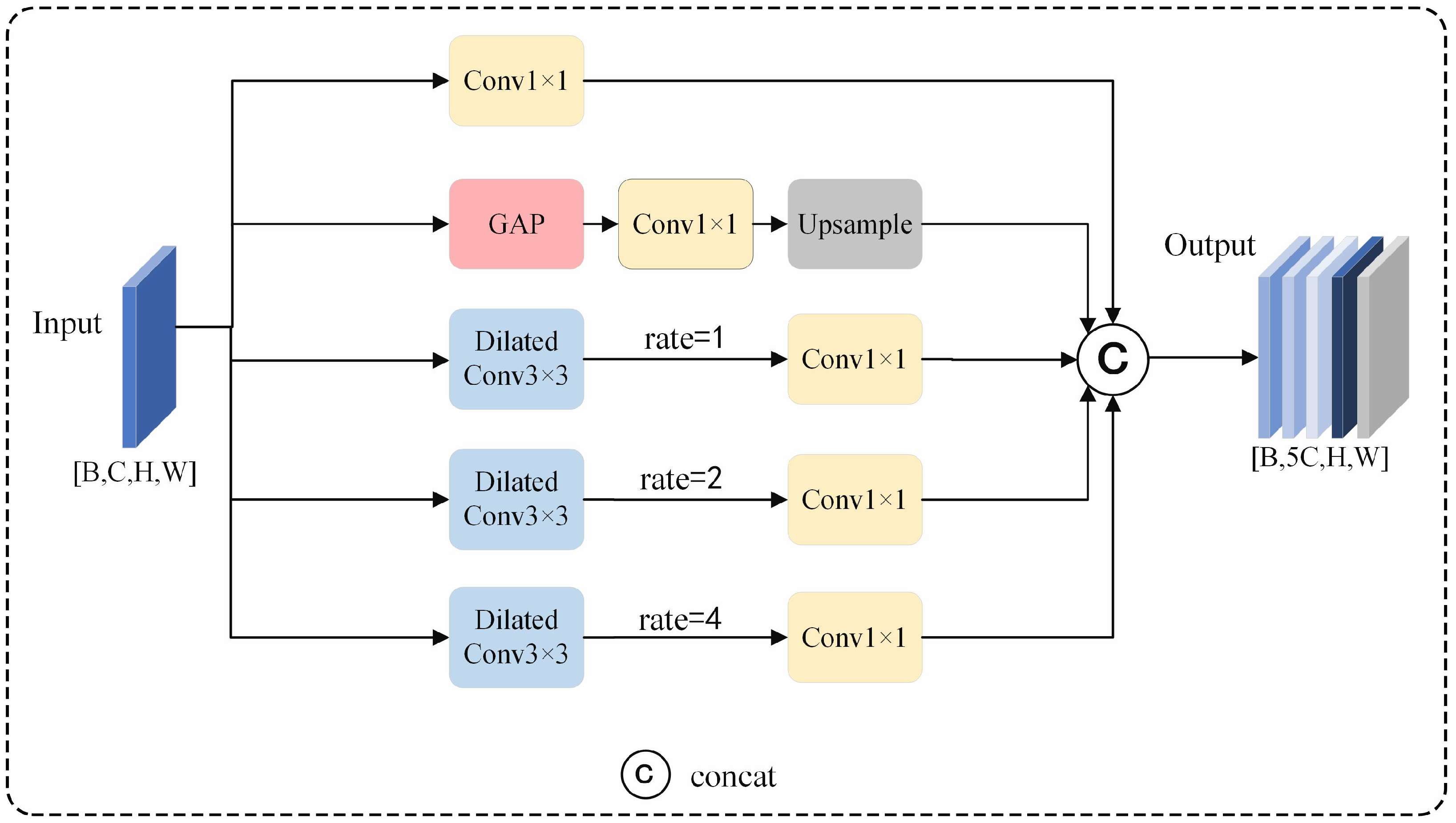
In remote sensing scenes characterized by complex terrain and highly heterogeneous snow distribution, snow depth estimation requires a strong capability to perceive features at multiple spatial scales. To effectively extract multi-scale contextual information from snow-covered areas and improve the model’s robustness in situations such as abrupt slope changes and patchy snow cover, we designed the Multi-scale Feature Perception Module (MFPM), whose architecture is shown in the Figure 9.

Figure 9. The architecture of the Multi-scale Feature Perception (MFPM) module.

The MFPM module enhances the model’s ability to represent multi-scale spatial features by fusing information streams from five different receptive fields. First, the module includes a 1 × 1 standard convolutional branch to extract local textures and edge features, preserving the most original spatial structure. Second, a global average pooling branch is designed to compress the input feature map into a global representation vector. This vector, processed through a 1 × 1 convolution and an upsampling operation, provides global-level semantic context, effectively enhancing global perception. Furthermore, the MFPM incorporates three dilated convolution branches, employing 3 × 3 dilated convolutions with dilation rates of 1, 2, and 4, respectively, each followed by a 1 × 1 convolutional layer. This design corresponds to modeling local edges, mid-scale structures, and large-scale contexts, constructing a multi-level feature representation from details to semantics.

Once the features extracted from the five parallel paths are consistent in their spatial dimensions, they are concatenated along the channel dimension to form a joint feature representation. This structure both maintains local detail and effectively integrates large-scale background semantics, demonstrating excellent adaptability across various complex snow distribution patterns.

4. Experiments

This section systematically validates the effectiveness and state-of-the-art performance of the proposed Terrain-Aware Cross-Modality Fusion Network (TACMF-Net) for snow depth estimation through a series of quantitative and qualitative experiments. Our evaluation is conducted from six perspectives: construction of the SAR branch and the introduction of terrain factors, dual-branch fusion, module ablation studies, data ablation analysis, multi-model comparative experiments, and in-situ visualizations.

4.1. Experimental Setup

All experiments in this study were conducted using the PyTorch2.1.0 deep learning framework on a workstation equipped with an NVIDIA GeForce RTX 4070 graphics card.We split all the sample data we have obtained into training and testing sets in a 4:1 ratio. We chose the Adam (Adaptive Moment Estimation) optimizer for its excellent convergence performance to improve training efficiency. We also employed data augmentation techniques, such as horizontal and vertical flipping, and batch normalization to prevent overfitting. The dataset was further divided for five-fold cross-validation, following the initial split into training and testing sets, to ensure the reliability of the experimental results.

Considering our computational resources and project requirements, we set the batch size to 64 and the maximum number of training epochs to 200. The initial learning rate was set to 0.0005 and was updated using a polynomial decay strategy, as described by the following formula:

$$\mathrm{lr}=\text{base\_lr}\times {\left(1-{\displaystyle \frac{\mathrm{epoch}}{\text{max\_epoch}}}\right)}^{\mathrm{power}},$$

(10)

where base_lr is the initial learning rate of 0.0005, max_epoch is the total number of training epochs (200), epoch is the current training epoch, and power, which controls the slope of the learning rate decay curve, is set to 0.9. For the loss function, we used Mean Squared Error (MSE) as the optimization target for the regression task. We also selected several other metrics to comprehensively evaluate the model’s performance, including Root Mean Squared Error (RMSE), Mean Absolute Error (MAE), Positive Mean Error (PME), Negative Mean Error (NME), coefficient of determination ($R^2$), and Mean Relative Error (MRE).

$$\begin{array}{cc}\hfill \mathrm{MSE}(y,\widehat{y})& ={\displaystyle \frac{1}{N}}\sum _{i=1}^N{({\widehat{y}}_i-y_i)}^2,\hfill \end{array}$$

(11)

$$\begin{array}{cc}\hfill \mathrm{MAE}(y,\widehat{y})& ={\displaystyle \frac{1}{N}}\sum _{i=1}^N|y_i-{\widehat{y}}_i|,\hfill \end{array}$$

(12)

$$\begin{array}{cc}\hfill \mathrm{RMSE}(y,\widehat{y})& =\sqrt{{\displaystyle \frac{1}{N}}\sum _{i=1}^N{(y_i-{\widehat{y}}_i)}^2},\hfill \end{array}$$

(13)

$$\begin{array}{cc}\hfill \mathrm{PME}& ={\displaystyle \frac{1}{p}}\sum _{i=1}^p({\widehat{y}}_i-y_i),\mathrm{for}{\widehat{y}}_i>y_i,\hfill \end{array}$$

(14)

$$\begin{array}{cc}\hfill \mathrm{NME}& ={\displaystyle \frac{1}{r}}\sum _{i=1}^r({\widehat{y}}_i-y_i),\mathrm{for}{\widehat{y}}_i<y_i,\hfill \end{array}$$

(15)

$$\begin{array}{cc}\hfill \mathrm{MRE}& ={\displaystyle \frac{1}{N}}\sum _{i=1}^N{\displaystyle \frac{|{\widehat{y}}_i-y_i|}{y_i}},\hfill \end{array}$$

(16)

$$\begin{array}{cc}\hfill R^2& ={\left[{\displaystyle \frac{N-1}{N}}\sum _{i=1}^n\left({\displaystyle \frac{y_i-\mu \left(y_i\right)}{\sigma \left(y_i\right)}}\right)\left({\displaystyle \frac{{\widehat{y}}_i-\mu \left({\widehat{y}}_i\right)}{\sigma \left({\widehat{y}}_i\right)}}\right)\right]}^2.\hfill \end{array}$$

(17)

Here, y represents the estimated snow depth value, while $\widehat{y}$ represents the actual snow depth value observed at the ground station, which serves as the label. N denotes the total number of data samples.

4.2. Single-Branch and Terrain Enhancement Experiments

To investigate the capability of SAR data in snow depth estimation and to validate the enhancing effects of terrain factors and the TPG module, we first constructed a single-branch SAR network and conducted experiments with the incremental introduction of variables. Initially, only single-channel SAR data was used. Subsequently, DEM (elevation), slope, and aspect were added in succession. Finally, two TPG modules were incorporated to model the terrain-guided attention mechanism.

The experimental results, as shown in Table 1, indicate that using SAR data alone resulted in significant errors (RMSE 9.891 cm, $R^2$ only 0.227). This suggests that although SAR possesses penetration capabilities, its ability to represent centimeter-level snowpack is limited, leading to large prediction errors and poor model fitting. After adding the DEM, the RMSE dropped significantly to 4.116 cm, and the $R^2$ increased to 0.862, demonstrating that elevation is a strong indicator for snow estimation. With the further addition of slope and aspect, the $R^2$ improved to 0.971, and the RMSE decreased to 1.876 cm. This enhanced the model’s ability to capture the terrain-dominated distribution of snow. The results show that terrain factors markedly improved the model’s performance in areas with complex topography, especially in regions with sharp slope changes and uneven local snow distribution, where the model’s snow depth perception was greatly enhanced. Finally, with the introduction of two TPG modules, the RMSE was further reduced to 1.622 cm, and the $R^2$ reached 0.975. The experiment proves that this module can improve prediction accuracy in high-altitude, steep-slope regions and enhance the network’s ability to express terrain-dominant factors. In this study, the TPG module was integrated into the low and mid-level layers of the SAR branch to modulate terrain-related feature channels. This mechanism, in synergy with residual blocks and fusion modules, helps build a more robust and generalizable snow depth estimation model.

Table 1. Starting from a single SAR channel and gradually adding channels, this table shows the performance evaluation of the single SAR branch with the incremental introduction of terrain factors. Arrows indicate whether lower (↓) or higher (↑) values are better.

Method	RMSE ↓	MAE ↓	${\mathit{R}}^2$ ↑
SAR	9.891	7.778	0.227
SAR+DEM	4.116	1.983	0.862
SAR+DEM+Slope	2.200	1.220	0.961
SAR+DEM+Slope+Aspect	1.876	0.940	0.971
SAR+DEM+Slope+Aspect+TPG	1.622	0.811	0.975

4.3. Branch Structure Experiments

We further compared the performance of the optical branch, the SAR branch, and the dual-branch fusion structure. Optical remote sensing provides richer spectral and textural information, while SAR remote sensing offers interference resistance and terrain penetration capabilities, making them clearly complementary. The experimental results show that the optical branch outperformed the SAR branch (RMSE of 0.649 vs. 1.622). However, the performance significantly improved after dual-branch fusion, with the RMSE dropping to 0.304 and the $R^2$ reaching 0.994, which validates the significant value of multi-modal synergistic modeling for snow depth estimation, as shown in Table 2.

Table 2. Performance comparison between single-branch (SAR, Optical) and dual-branch fusion structures. Arrows indicate whether lower (↓) or higher (↑) values are better.

Method	RMSE ↓	MAE↓	${\mathit{R}}^2$ ↑
SAR Branch	1.622	0.811	0.975
Optical Branch	0.649	0.347	0.988
Double Branches	0.304	0.213	0.994

4.4. Module Ablation Study

To systematically evaluate the contribution of each module within the dual-branch network, we incrementally added the Multi-scale Feature Perception (MFPM) and Cross-Modality Feature Fusion (CMFF) modules to the base model, designing four comparative experiments: the base dual-branch structure (Double Branches), introduction of two MFPM modules (Double+2MFPM), introduction of two CMFF modules with branch adjustment (Double+2CMFF), and the complete structure (Double+2CMFF+4MFPM, i.e., TACMF-Net). The results are presented in Table 3.

Table 3. Ablation study of different modules within the TACMF-Net architecture, showing the progressive improvement by adding MFEM, CMFF, and both modules combined. Arrows indicate whether lower (↓) or higher (↑) values are better.

Method	RMSE ↓	MAE ↓	${\mathit{R}}^2$ ↑	Params↓	FLOPs ↓
Double Branches	0.304	0.213	0.994	1.43 M	0.212 G
Double+2MFPM	0.282	0.191	0.995	1.65 M	0.221 G
Double+2CMFF	0.228	0.169	0.996	1.99 M	0.261 G
Double+2CMFF+4MFPM	0.216	0.154	0.997	2.35 M	0.279 G

The initial base model took optical and SAR images as input, extracted features using a symmetric residual structure, and finally fused them for regression. This structure, without any feature enhancement modules, already achieved high performance (RMSE = 0.304, $R^2$ = 0.994) but exhibited local overestimation or underestimation in complex terrain.

To enhance the model’s understanding of terrain semantics, we introduced one MFPM module at the end of each branch (total of 2), creating the Double+2MFPM model to fuse structural texture information from different receptive fields. After adding MFPM, the model’s RMSE decreased to 0.282, and the MAE dropped to 0.191, demonstrating the significant effect of multi-scale dilated convolutions in improving feature representation.

Furthermore, to enhance the cross-modality collaborative expression between the optical and SAR branches, we inserted one CMFF module after the first and second residual units in each branch to dynamically fuse local semantic features of the same scale from both modalities. This was followed by new residual structures to maintain feature dimension consistency, resulting in a four-branch collaborative structure (Double+2CMFF). This configuration, without the MFPM, reduced the RMSE to 0.228 and increased the $R^2$ to 0.996, indicating that the mid-level cross-modality fusion strategy effectively mitigated information inconsistency between modalities and improved the model’s discriminative ability.

Finally, by adding one MFPM module at the end of each of the four branches in the Double+2CMFF structure (total of 4), we obtained the complete TACMF-Net model. This architecture integrates mid-level cross-modal interaction with end-stage multi-scale feature aggregation, fully enhancing the model’s comprehensive perception of multi-source snow depth signals. The experiments showed that this model achieved optimal accuracy and robustness (RMSE = 0.216, MAE = 0.154, $R^2$ = 0.997), while its parameter count (2.35 M) and computational complexity (0.279 G FLOPs) remained within a manageable range, balancing high precision with practical efficiency.

4.5. Multi-Model Comparative Experiments

After the above model design, we obtained the final results. Compared with existing studies on snow depth estimation in high-latitude regions of Asia (such as MFPANet), the results are comparable, which validates the effectiveness of this model approach.

To comprehensively evaluate the practical performance of our proposed TACMF-Net in the task of snow depth estimation, we selected several representative deep learning models as a control group and conducted rigorous comparative experiments under a unified dataset and training strategy. The results are presented in Table 4. Key parameters (such as the initial learning rate and weight decay coefficient) are independently optimized through grid search on a unified validation set to ensure that each model reaches its optimal configuration. The compared models were mainly divided into two categories: (1) existing models in the field of snow depth estimation, including classics like DSDRNet [34] and ConvNet [25], as well as more recent models such as ResSD [13] and MFPANet [28]; and (2) general-purpose image recognition models, covering mainstream image classification and semantic segmentation networks like SENet [33], VGG-16 [35], ResNet series, DenseNet121 [36], MobileNetV2 [37], ShuffleNetV2 [38], Vision Transformer [39], and Inception [40]. To adapt these single-modality networks, we stacked all registered data to form an 8-channel image as input for the comparison models and replaced the output layer with a single-neuron regression head to predict the corresponding snow depth. During training, we used the same training set and tested on the same test set. Our evaluation metrics included RMSE, MAE, PME, NME, MRE, $R^2$, and the number of parameters.

Table 4. Performance Comparison of TACMF-Net Against 14 Benchmark Models on Our Dataset. Our model achieves state-of-the-art accuracy (RMSE: 0.216, MAE: 0.154) while maintaining parametric efficiency (2.36 M parameters), demonstrating significant superiority over comparative methods. Bold values indicate optimal performance. Arrows indicate whether lower (↓) or higher (↑) values are better.

Model	RMSE ↓	MAE ↓	PME ↓	NME ↑	MRE ↓	${\mathit{R}}^2$ ↑	Params ↓
DSDRNet	3.324	2.035	2.047	−2.024	0.199	0.914	164.50 k
ViT	0.999	0.508	0.489	−0.468	0.052	0.978	292.87 k
ConvNet	0.879	0.448	0.432	−0.422	0.048	0.979	26.64 k
DenseNet121	0.828	0.386	0.368	−0.385	0.044	0.981	7.04 M
VGG16	0.801	0.349	0.364	−0.369	0.046	0.983	14.79 M
ShuffleNetV2	0.718	0.385	0.386	−0.325	0.048	0.983	136.89 k
MobileNetV2	0.673	0.356	0.330	−0.312	0.042	0.985	2.31 M
Inception	0.513	0.293	0.312	−0.257	0.039	0.986	5.93 M
SENet	0.443	0.258	0.263	−0.253	0.030	0.988	0.69 M
Resnet34	0.411	0.236	0.253	−0.226	0.031	0.989	21.31 M
Resnet50	0.406	0.216	0.217	−0.225	0.031	0.989	23.64 M
ResSD	0.396	0.232	0.226	−0.248	0.029	0.990	689.60 k
Resnet18	0.374	0.222	0.184	−0.238	0.029	0.991	11.21 M
MFPANet	0.360	0.204	0.176	−0.230	0.026	0.992	13.61 M
Ours	0.216	0.154	0.146	−0.158	0.020	0.997	2.36 M

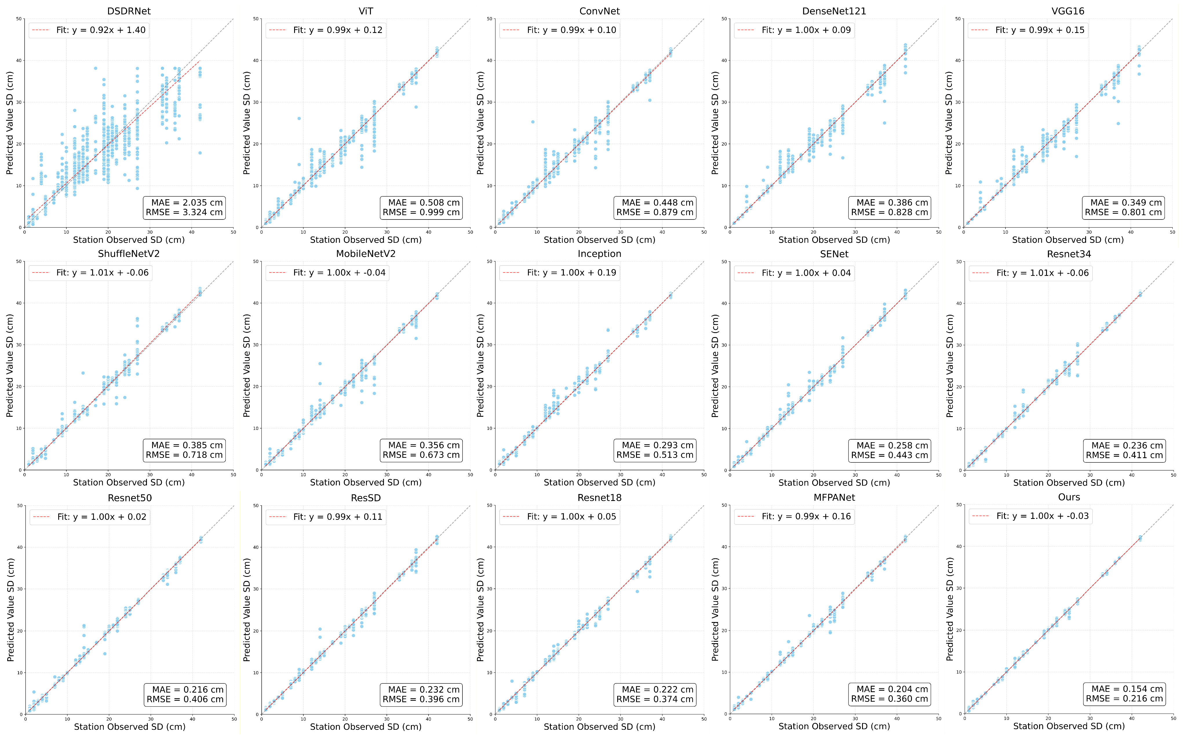
We performed regression fitting on the estimation results of each model on our terrain-remote sensing multi-source snow depth dataset. The experimental results, shown in Figure 10, indicate that different models performed variously. The prediction accuracy of some comparative models is poor, their robustness to data noise is insufficient, and they are prone to significant outlier errors. Models that perform poorly display more scattered points visually, whereas models that perform well have points concentrated near the line y = x, resulting in fewer visible points due to overlap. Traditional convolutional architectures (such as DSDRNet and ConvNet) possess a certain degree of generalization ability, but their relatively shallow network depth and limited receptive field constrain the extraction of deep semantic features in complex snow depth distributions in remote sensing imagery. Deep residual networks, represented by the ResNet series, effectively alleviate the vanishing gradient problem, enabling the construction of deeper networks and the extraction of richer features. However, they still exhibit significant bias in estimating medium snow depth ranges (20–30 cm), which may stem from their insufficient capacity to model multi-scale snow features and their nonlinear interactions with terrain. The latest snow depth estimation networks (such as ResSD and MFPANet) have made notable progress, yet their performance remains limited by two factors: first, they fail to leverage the modulating effect of key terrain factors (such as elevation and slope); second, there is still room for improvement in the efficiency of integrating multi-source remote sensing data. The experimental results clearly show that our model outperformed other algorithms across all metrics. As seen from the fitting plots, our predictions are highly accurate, with an RMSE of only 0.216 and an MAE of 0.154, and a parameter count of just 2.36 M. Its fusion of the terrain-aware module and cross-modality guidance mechanism enables the model to not only exhibit superior performance at a global scale but also provide stable estimations across different depth ranges.

Figure 10. Two-dimensional scatter plots comparing estimated versus measured snow depth across different models, with Root Mean Square Error (RMSE) and Mean Absolute Error (MAE) metrics annotated for each method. The gray dashed line denotes the ideal 1:1 reference line (y = x), while red solid lines represent actual regression trends of respective models. Results demonstrate that our method (marked with red pentagrams) exhibits the closest alignment with the reference line, showing statistically significant superiority over comparative models.

The reason such high accuracy can be achieved is that multi-source data collaboratively provide complementary information. Although single-source data has limited resolution, nonlinear fusion and cooperative interpretation of multi-source features through deep learning models can significantly reduce the uncertainty of a single sensor, thereby statistically constraining higher-precision snow depth estimates. It should be noted that the model does not directly ‘see’ centimeter-level changes from 10-m pixels; rather, it learns from a large number of training samples the complex mapping relationships between snow depth and features such as multispectral data and terrain. When these features exhibit regular combinations under specific terrain and weather conditions, the model can infer centimeter-level differences in snow depth.

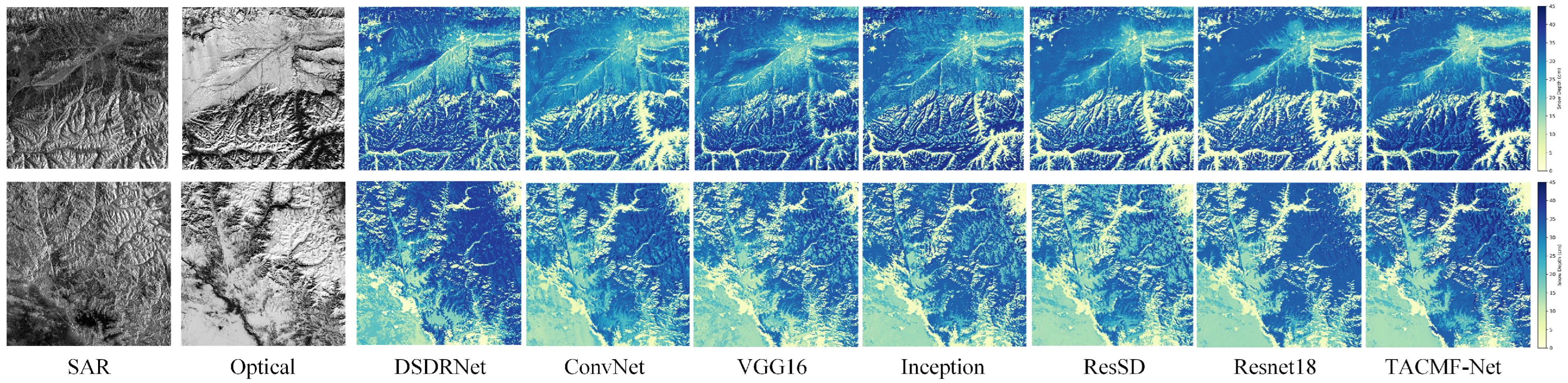
Subsequently, we selected multi-source remote sensing images and terrain data from the Zhaosu and Fuyun stations in Xinjiang. Based on the performance in the above comparative experiments, we chose six models—DSDRNet, ConvNet, VGG16, Inception, ResSD, and ResNet18—along with our model to perform large-scale, high-resolution snow depth mapping. As shown in Figure 11, the traditional model ConvNet exhibited a clear “snow depth collapse” phenomenon, where the prediction map appeared pale, and snow depth values were generally underestimated, especially in deep snow areas. The ResSD model, while showing a better overall trend, still had misjudgments in some edge areas and produced blurred predictions with abrupt spatial transitions in terrain-sensitive valleys. In contrast, our TACMF-Net demonstrated excellent spatial coherence in multiple regions. The estimated values showed a continuous transition between ridgelines and slope foots, and the color gradations in the map were distinct with high detail fidelity, accurately capturing the snow accumulation patterns controlled by topography. The model accurately depicted the fact that snow does not easily accumulate on ridges, and the resulting prediction map showed high consistency with the shape and boundaries of the terrain imagery.

Figure 11. Different models were used for snow depth mapping at Xinjiang’s Zhaosu Station and Fuyun Station. Based on the comparison of model performance, six models—DSDRNet, ConvNet, VGG16, Inception, ResSD, and ResNet18—were selected along with our proposed model for large-scale high-resolution snow depth mapping. In contrast, our model’s depiction of snow-covered scenes aligns more closely with the actual distribution, and the predicted maps exhibit highly consistent shape contours and boundaries with the topographic imagery.

To further evaluate the model’s prediction performance across different snow depths, we divided the samples into four depth intervals based on the ground station label values: 1–10 cm, 10–20 cm, 20–30 cm, and greater than 30 cm, and calculated the RMSE and MAE within each interval. The results are presented in Table 5. The results indicate that the model performed best in shallow snow regions (1–20 cm) with small estimation errors. The error increased slightly in the 20–30 cm range, primarily due to a smaller number of samples and a more patchy and heterogeneous snow distribution. In deep snow areas (>30 cm), TACMF-Net maintained stable performance, demonstrating its good generalization capability and strong response to high snow depths.

Table 5. Performance of TACMF-Net across different snow depth ranges. Arrows indicate that lower (↓) values are better.

Depth Range (cm)	RMSE ↓	MAE ↓
1–10	0.207	0.144
10–20	0.212	0.149
20–30	0.231	0.161
>30	0.220	0.157

4.6. Generalization Test

To test model generalization, we utilized a separate set of four meteorological stations that were completely independent of the training data. Specifically, the Zhaosu and Nilka stations are located in the high mountain and hilly zone on the periphery of the Ili River Valley, characterized by intense topographic relief and significant slope variations, representing typical complex terrain snow distribution areas. In contrast, the Tacheng and Habahe stations are situated in the low mountain-to-basin transition zone on the southern edge of the Altai Mountains, with relatively gentle overall topography and minor structural changes.

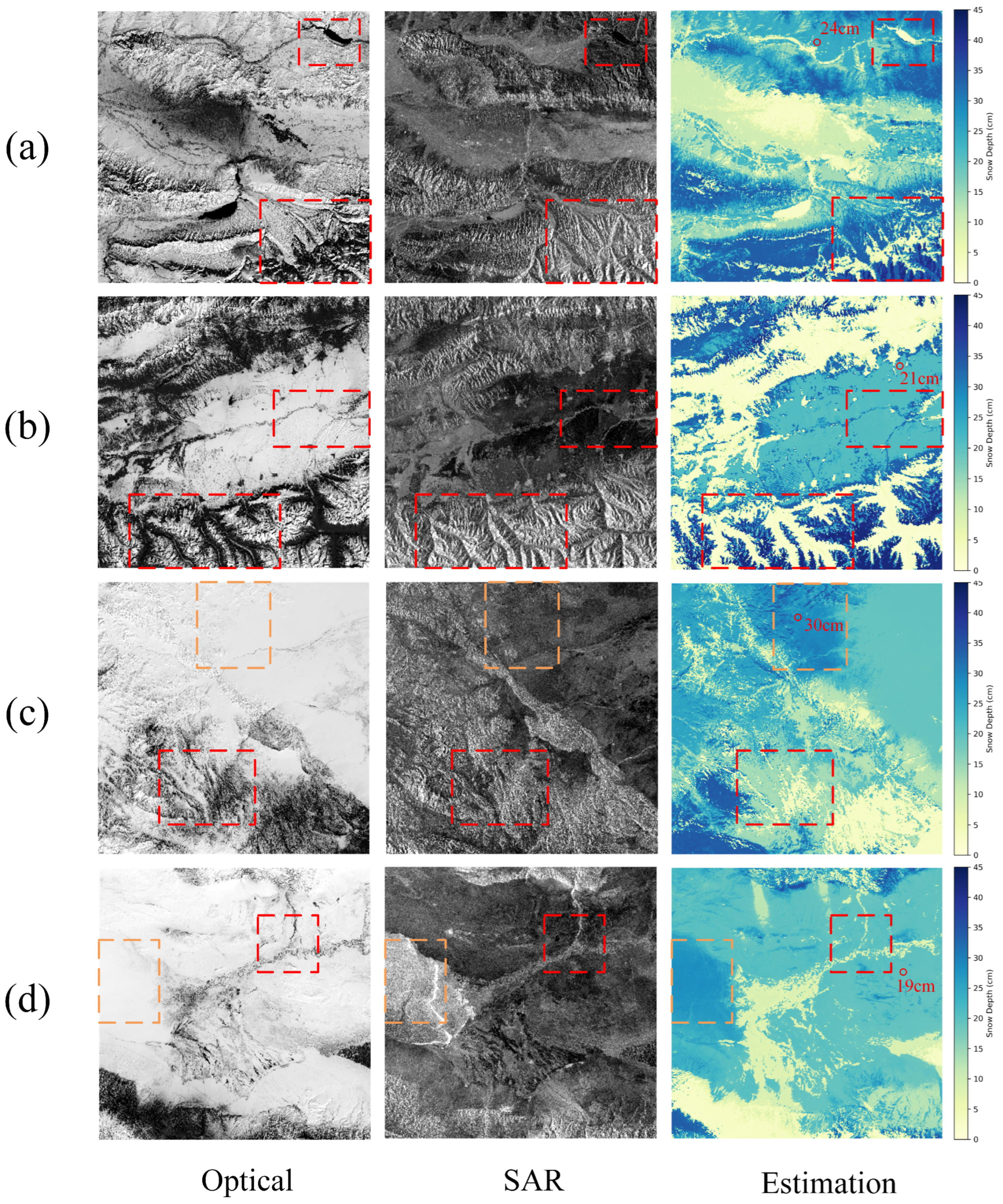
We can observe that in these complex terrain regions, the snow depth distribution maps generated by TACMF-Net exhibit extremely strong spatial awareness and detail-rendering capabilities. As highlighted by the red boxes in Figure 12a,b, the model is able to accurately identify variations in snow accumulation and sparseness caused by micro-topographic differences along ridges, valleys, and north-south facing slopes. For instance, in higher-elevation, steeper valley areas, the model predicted significantly deeper snow than on adjacent slopes, which is highly consistent with real-world snow distribution. The color bands also showed a natural top-to-bottom transitional hierarchy, without any “boundary fractures” or “blurred snow patches.”

Figure 12. Demonstration of TACMF-Net’s spatial generalization capability. (a) Zhaosu station; (b) Nilka station; (c) Tacheng station; (d) Habahe station. We use pixel color variations from light yellow to dark blue to represent snow depth ranging from 0–45 cm. The red circle represents the location of the station. The red value denotes the measured snow depth value of the station on the day.

In contrast, in flat areas with little terrain variation, the snow depth maps generated by TACMF-Net still maintained high consistency and stability. The areas around the Tacheng and Habahe stations are open with gentle slopes and weak surface texture information; as highlighted by the red boxes in Figure 12c,d, this environment often poses a greater challenge to a model’s feature recognition capabilities. Nevertheless, TACMF-Net was still able to clearly predict the edges of the snowpack, with results that were highly consistent with the measured values. In areas of generally uniform snow distribution within Figure 12c,d, such as the sections highlighted by the orange boxes, the model could still identify patchy structures with slightly deeper snow in local areas. This level of detail further confirms that TACMF-Net has a distinct advantage in resolving micro-scale surface differences.

In summary, TACMF-Net demonstrated excellent snow depth estimation capabilities in both types of typical terrain. In rugged mountainous areas, its structural understanding and multi-scale fusion abilities enabled it to accurately model snow distribution under complex topography. In flat regions, it showed good stability and consistency, avoiding the risk of misjudgment from “over-reliance on boundary information”.

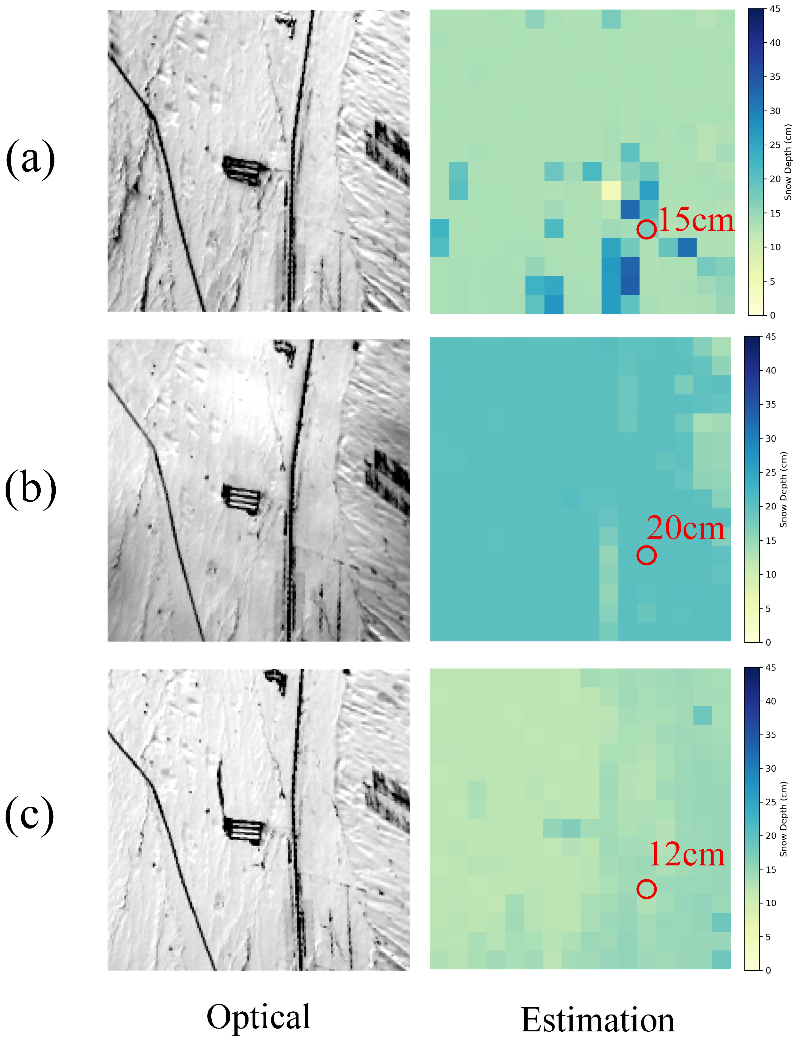
For the time dimension, we additionally reselected and downloaded three sets of remote sensing images from the Toli Station in Xinjiang, which represent the local snow depth at Toli Station on 3 January, 4 February, and 27 February 2015, from top to bottom. From the images, we can clearly see that within an interval of a month and a half, our model correctly measured different snow depths, indicating that our model can effectively detect snow of varying depths and its changing trends, as shown in Figure 13.

Figure 13. (a) Tori station on 3 January 2015; (b) Tori station on 4 February 2015; (c) Tori station on 27 February 2015. The red circle represents the location of the station, and the red value denotes the measured snow depth value of the station on the day.

4.7. Data Ablation Analysis

To systematically verify the specific contributions of various remote sensing data sources to the snow depth estimation task, we conducted data ablation experiments. By selecting a representative model architecture, ResNet18, and constructing different combinations of input channels, we evaluated the impact of single or partial data sources on model performance. The specific setups included: (1) using only SAR images and terrain features extracted from DEM (denoted as SAR+DEMect); (2) using optical images and DEMect; (3) using optical and SAR images; and (4) using all three data types to form an 8-channel input (Optical+SAR+DEMect).

As shown in Table 6, the combination of SAR+DEMect alone yielded a high RMSE of 3.768 and an $R^2$ of only 0.884, indicating that even with the inclusion of terrain factors, the lack of optical information made it difficult for the model to fully perceive the details of snow distribution. The Optical+DEMect combination reduced the RMSE to 0.445, demonstrating the strong advantage of optical information in representing surface texture and spatial structure. Further combining SAR and optical images (Optical+SAR), the RMSE decreased to 0.413 and the $R^2$ increased to 0.988, which shows that different remote sensing modalities have good complementarity and can improve the model’s understanding and modeling of snow depth information. Notably, when all three data types were fused into an 8-channel input (Optical+SAR+DEMect), the model performance reached its optimum (RMSE = 0.374, $R^2$ = 0.991), significantly outperforming other combinations. This validates the importance of terrain information for model detail optimization and snow depth transition perception and further supports the rationale behind introducing the Terrain-Aware Guidance (TPG) module and the Cross-Modality Feature Fusion (CMFF) structure in our backbone network design.

Table 6. Performance evaluation of different data source combinations using the ResNet18 backbone. Arrows indicate whether lower (↓) or higher (↑) values are better.

Data Combination	RMSE ↓	MAE ↓	${\mathit{R}}^2$ ↑	Channels
SAR+DEMect	3.768	1.731	0.884	4
Optical+DEMect	0.445	0.258	0.986	7
Optical+SAR	0.413	0.239	0.988	5
Optical+SAR+DEMect	0.374	0.222	0.991	8

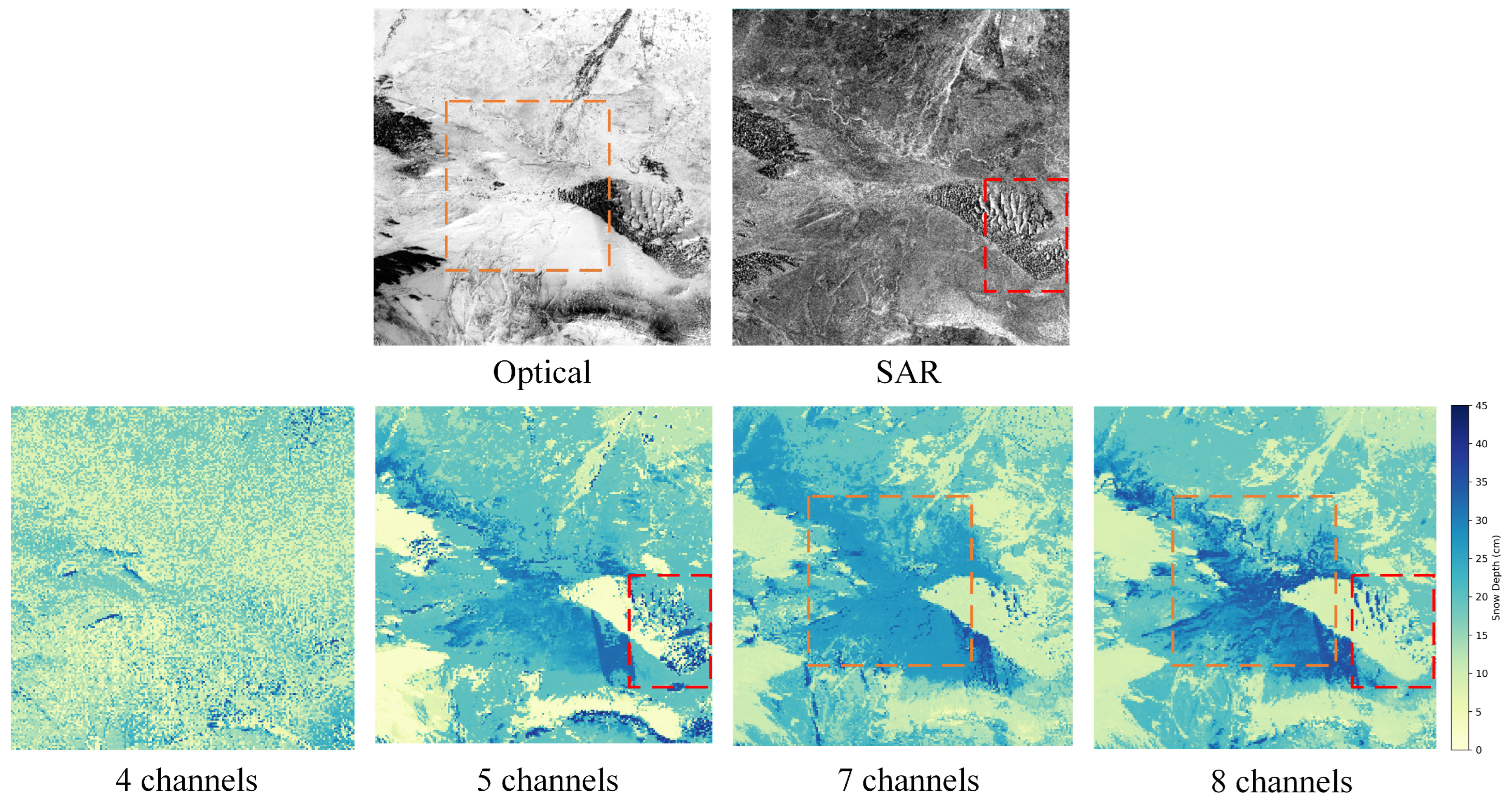
To intuitively demonstrate the impact of different data combinations on the spatial estimation results, Figure 14 presents the snow depth estimation maps for the four input combinations in the same region. The figure clearly shows that with only SAR+DEMect input, the model’s prediction map exhibits large areas of “blurry, clumpy” snow distribution, lacking clear edges and spatial structure, which results in significant misjudgments; this indicates that a lack of optical spatial features hinders the model’s ability to identify the actual snow pack outline. The Optical+DEMect combination preserved edge structures to some extent but showed significant overestimation or underestimation in several key areas, as highlighted by the orange boxes in Figure 14. Especially in valley regions, the snow depth values widely deviated from the measured values. This suggests that relying solely on optical reflectance properties without support from internal structural features can easily lead to estimation biases and weak generalization, and although the $R^2$ increased to 0.986, the local performance was unstable. In the Optical+SAR combination’s prediction results, spatial coherence was markedly improved, and the structure and distribution of snowpack were more realistic. However, the expression of snow depth gradients is insufficient in areas of intense topographic relief, as highlighted by the red boxes in Figure 14, where local terrain-controlled features are somewhat missing, reflecting a lack of additional spatial constraints for complex terrain. Finally, the image produced by fusing Optical, SAR, and DEMect most closely resembled the actual terrain variations; the model could not only accurately delineate the snow depth gradients corresponding to micro-topographic features such as ridges and valleys but also distinguish between high-snow-depth accumulation zones and sparse areas, with sharp edges and natural transitions, demonstrating extremely strong spatial representation capabilities.

Figure 14. Visual comparison of snow depth maps generated from different data source combinations.

From Table 6, it can be seen that for our research on snow depth estimation, the most important features are optical features, followed by SAR features and DEM-related features. The introduction of terrain factors not only enhanced the model’s sensitivity to spatial distribution structures but also improved its robustness in complex terrain. The complementarity of SAR and Optical data provided dual support in both semantics and structure, ensuring a reliable basis for high-precision snow depth estimation.

5. Conclusions and Future Work

This paper has focused on the problem of snow depth estimation in high-altitude, complex terrain regions, proposing a deep learning model that fuses multi-source remote sensing information with terrain-based prior knowledge—TACMF-Net (Terrain-Aware Cross-Modality Fusion Network). The model fully leverages the complementary strengths of optical and SAR remote sensing data in terms of textural features and structural penetration. It enhances its expressive capability for different snow depth levels through the Terrain-Aware Guidance (TPG) module and the Multi-scale Feature Perception (MFPM) module. Furthermore, the proposed Cross-Modality Feature Fusion (CMFF) module effectively coordinates the semantic information between the optical and SAR branches, achieving a deep level of information guidance and reconstruction. In a series of ablation studies, visual analyses, and comparative experiments, TACMF-Net outperformed existing methods on key metrics such as RMSE, MAE, and $R^2$, particularly demonstrating superior stability and generalization capability in regions characterized by high mountains, hills, and complex patchy snow distributions. Through comparisons with several mainstream snow depth estimation networks and image recognition architectures, we have verified that TACMF-Net achieves an excellent balance between accuracy, robustness, and model complexity, possessing strong potential for practical deployment. Concurrently, the data-level ablation studies clearly demonstrate that optical, SAR, and terrain factors are all indispensable; only with the thorough fusion of this information can the model comprehensively and precisely perceive the spatial patterns of snow depth.

However, it should be noted that due to the difficulty of data production, our study only focuses on certain high-latitude regions in Asia, and the snow depth values in these areas are generally below 50 cm. Therefore, our experimental results only represent our study regions. In the future, we need to continuously expand our dataset, introduce more regions, and include data samples with greater snow depth values, as well as adjust our model to accommodate more regions and deeper snow, thereby enhancing generalization capability and making our research more comprehensive. Although TACMF-Net has achieved leading performance on multiple metrics, we still need to be cautious of the risk of overfitting. Additionally, the current model primarily performs snow depth estimation based on static remote sensing images. Future work could consider incorporating time-series modeling structures (such as ConvLSTM or Transformers) to achieve dynamic modeling and prediction of snowpack evolution. Then, with regard to spatial resolution, as the availability of high-resolution optical and SAR data improves, future research could focus on designing finer-grained feature extraction modules to address the demands of sub-meter-level snow depth estimation. At the deployment level, lightweight model modifications, model distillation, and adaptation for edge computing will be crucial directions for transitioning this method to operational use at in-field snow monitoring stations. In summary, TACMF-Net not only provides an innovative solution for snow depth estimation under complex terrain conditions but also offers a methodological paradigm for multi-modal remote sensing fusion research, possessing significant scientific value and practical application prospects.