Non-Linear Method of Vehicle Velocity Determination Based on Tensor Product B-Spline Approximation with Probabilistic Weights for NHTSA Database of Compact Vehicle Class

Abstract

This research article focuses on the method of vehicle crash velocity evaluation based on the tensor product approximation by B-splines. Weights associated with each observation are introduced in the least square method, which is based on probabilistic reasoning. The presented calculation algorithm is built based on the Compact vehicle class from the NHTSA database, which consists of 338 records of frontal crashes with stationary obstacles. The presented model is restricted to velocities in the range between 43 and 93.5 km/h. The relative error obtained for the presented calculation method is 5.2%. Hence, improvement has been observed in comparison with the linear model with the same probabilistic weights approach, for which relative error is equal to 5.47%.

1. Introduction

In order to perform a crash reconstruction, it is necessary to estimate pre-impact conditions as reliably as possible. This is usually accomplished on the basis of both physical evidence and experimental or numerical crash data. Over the last decades a wide range of reconstruction methodologies have been developed, including approaches based on full scale crash tests, numerical simulation, and statistical analysis of accident databases [1,2,3]. Large experimental programs and case studies have provided reference data for different vehicle classes and impact configurations and have shaped current practice in road accident reconstruction [4,5,6]. These works emphasize that any realistic reconstruction must take into account vehicle structure, impact configuration, and post-impact motion, and that systematic methods are needed to relate measured deformations to pre-crash velocity [7,8,9].

In cases where a stationary obstacle is involved, as in this research, the deformation work is equal to the kinetic energy loss during the collision. Thus, it can be concluded that the theoretical velocity before impact is equal to (1):

$$V_r=\sqrt{{\displaystyle \frac{2W}{m}}} [\mathrm{m}/\mathrm{s}]$$

(1)

whereas

• $V_r$ denotes the vehicle velocity in the moment of the impact,
• $W$ is the work of deformation $\left[\mathrm{J}\right]$,
• $m$ denotes the car mass $\left[\mathrm{k}\mathrm{g}\right]$.

A commonly used framework for this purpose is the energy-based approach, in which the concept of equivalent energy speed (EES) is employed to link the energy absorbed in deformation to the change in vehicle kinetic energy [10,11,12], yielding $V_r\simeq V_t$, the observable pre-crash velocity, thus linking the vehicle deformation to its observable speed. Within this framework a number of authors have proposed procedures for estimating energy loss in frontal and oblique collisions, as well as for deriving impact velocity from residual crush [13,14,15]. In many practical implementations the relationship between EES and a chosen deformation measure is assumed to be linear, which simplifies calculations and allows one to calibrate models directly from crash test data [16,17,18]. The deformation coefficient $C_s$, defined on the basis of several measurement points distributed over the vehicle front, is one of the key quantities used in such models and has been discussed in detail in the context of reconstruction practice [19,20,21]. At the same time, studies of vehicle motion and impact dynamics show that local stiffness variations, structural non-linearity and post-impact kinematics can introduce significant deviations from simple linear relationships [22,23,24].

Beyond the standard stiffness-based calibration framework, additional deformation-driven estimators have been proposed that exploit richer information extracted from the damaged vehicle front. In particular, the deformation work has been modeled directly as a function of the deformation ratio using class-specific correlation schemes, and impact speed has been inferred from a geometric approximation of the deformed vehicle-body plane constructed from multiple measurement points [25,26]. These contributions underline that the accuracy of EES-based reconstruction depends critically on how residual crush is parameterized and motivates the use of flexible non-linear models when the linear assumption becomes insufficient.

In response to these limitations, more advanced modeling strategies have been explored. These include inverse system formulations, in which the mapping from deformation to velocity is treated as the inverse of a dynamic model [27,28,29]. Other authors have investigated polynomial and related functional approximations that attempt to capture non-linear crash behavior beyond simple straight-line fits [30,31,32]. More recently, further extensions and refinements of these ideas have been proposed, including higher order representations and variants tailored to specific impact configurations [33,34,35]. Related contributions, including the authors’ own previous work and independent studies, demonstrate that combining detailed crash test data with more flexible mathematical models can lead to a noticeable reduction in reconstruction errors and provide a better description of complex impact scenarios [36,37,38,39,40]. These developments highlight the potential of non-linear models, but they also show that many existing approaches still treat all observations as equally dependable, which makes them sensitive to outliers and biased sampling.

The methodological aim of this paper is to construct a precise and robust non-linear model for pre-crash velocity that accounts for the varying credibility of tests. This addresses a narrow research gap, as most existing Equivalent Energy Speed (EES)-based reconstruction methods rely on simple linear relationships between EES and deformation ratio, or on unweighted polynomial and inverse system approximations. Such conventional approaches treat all observations equally and are therefore sensitive to outliers and biased sampling. In this paper, another method is proposed, which enables determining vehicle velocity just before the collision. This method is based on the tensor product approximation, which furthermore incorporates probabilistic weights. The latter are included to explicitly account for test typicality and improve robustness to outliers. By integrating tensor product B-splines with a data-driven measure of observation typicality, the proposed approach offers a flexible yet interpretable alternative that improves predictive accuracy and robustness. As a result, the article contributes to the development of more reliable tools for accident reconstruction and forensic engineering and provides a methodological framework that can be transferred to other vehicle classes and crash configurations.

2. Materials and Methods

Before proceeding with the general method description, the most prominent features of the considered dataset are described. Therefore, in Section 2, we discuss the NHTSA Compact class crash test database that forms the empirical basis of the study. Basic descriptive statistics are provided for vehicle mass, deformation coefficient $C_{s,}$ and impact velocity $V_t$, as well as the practical limitations it imposes on the admissible velocity range. The uneven and partially clustered structure of the data is highlighted, along with the presence of outliers, which motivates the use of methods that are robust to non-uniform sampling and atypical observations. Next, the main definitions and properties of univariate B-splines are recalled. What follows is an explanation why their local support, smoothness, and partition of unity properties make them particularly suitable for approximating the non-linear relationship between deformation and pre-crash velocity. Finally, introduction of the tensor product B-spline approximation with probabilistic weights is in order. Each crash test is assigned a weight reflecting how typical it is with respect to the empirical distribution. Subsequently the corresponding weighted least squares problem is formulated, that will be used to estimate the model parameters.

2.1. Dataset Description

Our model is restricted to velocities in the range between $12$ and $26 \mathrm{m}/\mathrm{s}$. These limitations are a direct outcome of the utilized dataset limitations. As previously mentioned, the dataset used in this paper consists of 338 records. $20\mathrm{\%}$ of them were set aside for validation/test purposes. A brief description of the dataset along with its base characteristics is included in Table 1.

Table 1. Basic statistical characteristics of data.

$\mathit{S}\mathit{t}\mathit{a}\mathit{t}\mathit{i}\mathit{s}\mathit{t}\mathit{i}\mathit{c}$	$\mathit{M}\mathit{a}\mathit{s}\mathit{s}$ [kg]	${\mathit{C}}_{\mathit{s}} \left[\mathbf{m}\right]$	${\mathit{V}}_{\mathit{t}} [\mathbf{m}/\mathbf{s}]$
$mean$	1364.729	0.456	14.679
$standard$ $deviation$	61.090	0.142	2.574
$min$	1251	0.103	4.472
$Q_{25\%}$	1324	0.362	13.222
$Q_{50\%}$	1363	0.455	15.500
$Q_{75\%}$	1410.5	0.543	15.694
$max$	1478	1.328	26.861

The structure of the dataset indicates quite uneven distribution, which can be seen in Figure 1 and Figure 2. We can clearly see some deviating observations outside of the general surface. This plot shows the three-dimensional distribution of the impact velocity $V_t$ as a function of the vehicle mass and the deformation coefficient $C_s$. Most of the points are concentrated in a relatively narrow region of the space: masses of about $1300\text{–}1450 \mathrm{k}\mathrm{g}$, $C_s$ values roughly in the range $0.4\text{–}1.2 \mathrm{m}$, and impact velocities of about $15\text{–}20 \mathrm{m}/\mathrm{s}$. This means that the test database is richest precisely in this typical range of parameters, while there are considerably fewer observations corresponding to smaller or larger vehicle masses, extreme $C_s$ values, or very low and very high $V_t$ values. The cloud of points takes the form of a slightly inclined “band”, which suggests the existence of a relatively smooth, almost linear relationship between the impact velocity and the remaining variables $\left(Mass, C_s\right).$ The influence of mass appears rather small, whereas changes in the coefficient $C_s$ are associated with a more pronounced trend in $V_t$. At the same time, several tests lie clearly outside the main data cloud—they correspond both to unusually low (below about 10 m/s) and very high (above about 25 m/s) impact velocities. Such outlying observations confirm the uneven distribution of the data and may significantly affect the fit of classical regression models, which justifies the use of methods that are more robust to the presence of outliers and to the non-uniform sampling of the input space.

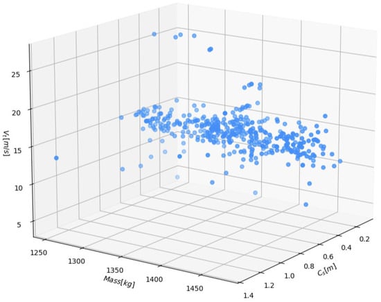
Figure 1. A scatterplot of observations within the dataset.

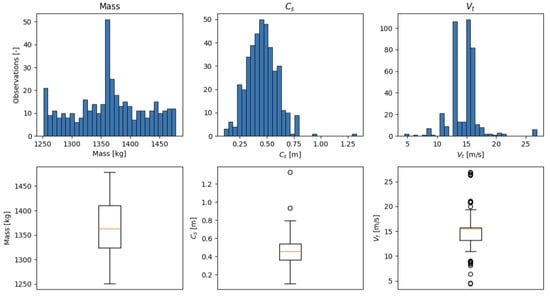
Figure 2. Distribution characteristics for each variable.

In summary, the available crash tests cover a relatively narrow and unevenly sampled region of the input space, with most cases corresponding to medium vehicle masses, moderate deformation coefficients, and impact velocities between $15$ and $20 \mathrm{m}/\mathrm{s}$. Only a small fraction of the data represents exceptionally low or remarkably high velocities and extreme $C_s$ values, and several clearly outlying observations are present. Consequently, the proposed model is calibrated and valid only within the velocity range of $12\text{–}26 \mathrm{m}/\mathrm{s}$, and any regression procedure must account for both the nonuniform density of the data and the influence of outliers, motivating the use of weighted and more robust modeling techniques in the subsequent sections. More detailed visual exposure for each variable is presented in Figure 2.

2.2. B-Splines and Their Properties

In the proposed approach, the relationship between the considered variables is modeled by means of B-splines. B-splines constitute a flexible family of piecewise polynomial basis functions that are widely used in approximation theory, numerical analysis, and computer-aided geometric design. Their main advantages include local support, good smoothness properties, and numerical stability, which make them particularly suitable for approximating non-linear dependencies observed in experimental data. In contrast to global polynomial bases, a local modification of the data affects only a limited number of neighboring basis functions, which is an important feature when working with measurement noise and outliers. Let ${\left({\mathit{x}}_{\mathit{i}}\right)}_{\mathit{i}=1}^{\mathit{l}}$ be a set of nodes. First, we define a B-spline of order 0 as follows (2):

$${\mathit{B}}_{\mathit{i}}^0(\mathit{x})=\left\{\begin{array}{c}1 \mathbf{if} x\in \left[{\mathit{x}}_{\mathit{i}},{\mathit{x}}_{\mathit{i}+1}\right),\\ 0 \mathbf{otherwise.} \end{array}\right.$$

(2)

From the mathematical viewpoint, these can be perceived as a characteristic function of respective intervals $[{\mathit{x}}_{\mathit{i}},{\mathit{x}}_{\mathit{i}+1})$. The recursive formula (see [41], p. 90), which is credited to Cox de Boor, allows us to construct B-splines of a higher order (3):

$${\mathit{B}}_{\mathit{i}}^{\mathit{d}}\left(\mathit{x}\right)={\displaystyle \frac{\mathit{x}-{\mathit{x}}_{\mathit{i}}}{{\mathit{x}}_{\mathit{i}+\mathit{d}}-{\mathit{x}}_{\mathit{i}}}}{\mathit{B}}_{\mathit{i}}^{\mathit{d}-1}\left(\mathit{x}\right)+{\displaystyle \frac{{\mathit{x}}_{\mathit{i}+\mathit{d}+1}-\mathit{x}}{{\mathit{x}}_{\mathit{i}+\mathit{d}+1}-{\mathit{x}}_{\mathit{i}+1}}}{\mathit{B}}_{\mathit{i}+1}^{\mathit{d}-1}\left(\mathit{x}\right), \mathit{d}\ge 1$$

(3)

There are several important properties of B-splines, which are worth mentioning. For instance, ${\mathit{B}}_{\mathit{i}}^{\mathit{d}}\left(\mathit{x}\right)>0$ for all $\mathit{x}\in [{\mathit{x}}_{\mathit{i}},{\mathit{x}}_{\mathit{i}+\mathit{d}+1})$. Simultaneously, ${\mathit{B}}_{\mathit{i}}^{\mathit{d}}\equiv 0$ outside of this interval.

Moreover, the set of all B-splines of order $\mathit{d}$ form a partition of unity [41] on the interval $[{\mathit{x}}_{\mathit{d}},{\mathit{x}}_{\mathit{l}-\mathit{d}})$, i.e., (4)

$${\sum }_{\mathit{i}}{\mathit{B}}_{\mathit{i}}^{\mathit{d}}\left(\mathit{x}\right)=1 \mathbf{f}\mathbf{o}\mathbf{r} \mathit{x}\in [{\mathit{x}}_{\mathit{d}},{\mathit{x}}_{\mathit{l}-\mathit{d}})$$

(4)

It is also noteworthy that there is a close relationship between the number of knots, the degree of B-splines, and their number, which can be formulated as (5):

$$\mathit{n}\mathit{r}\_\mathit{o}\mathit{f}\_\mathit{s}\mathit{p}\mathit{l}\mathit{i}\mathit{n}\mathit{e}\mathit{s}=\mathit{n}\mathit{r}\_\mathit{o}\mathit{f}\_\mathit{k}\mathit{n}\mathit{o}\mathit{t}\mathit{s}-\mathit{d}\mathit{e}\mathit{g}\mathit{r}\mathit{e}\mathit{e}\_\mathit{o}\mathit{f}\_\mathit{s}\mathit{p}\mathit{l}\mathit{i}\mathit{n}\mathit{e}\mathit{s}.$$

(5)

For example, if we require $7$ splines of degree $3$, then we need exactly $10$ nodes. To summarize, in this subsection we recalled the basic definitions and properties of univariate B-splines that will be used in the subsequent modeling. Starting from characteristic functions of consecutive intervals, higher-order B-splines are constructed by the means of Cox de Boor recursion, which yields non-negative basis functions with compact support. These functions form a partition of unity on the considered interval, which guarantees good numerical behavior and facilitates interpretation of the resulting approximation. We also emphasized the simple relationship between the number of knots, the spline degree, and the number of basis functions, which is essential when selecting an appropriate spline configuration for a given dataset.

2.3. Approximation Using Tensor B-Spline Products with Probabilistic Weights

We assume to have a given set of points ${\left(x_i,y_i,z_i\right)}_{i=1}^N$ and for each one of them we have defined the weight $w_i\in \left[\mathrm{0,1}\right]$, which determines its importance. Lower values of weight $w_i$ correspond to lower importance and zero value suggests that the point is discarded throughout the training process. Suppose that we also have a family of $M$ distinct functions $h_k:{\mathbb{R}}^2\to \mathbb{R}$, $k=1,\dots , M$ that we want to use to approximate our data points with. We want to utilize weighted least squares method, which is defined as minimizing the following loss function via modifying the coefficients ${\alpha }_k$ (6):

$${\sum }_{i=1}^N{w}_i{\left(z_n-{\sum }_{k=1}^M{\alpha }_k{h}_k\left(x_i,y_i\right)\right)}^2.$$

(6)

The problem of assigning weights is actually the easiest part of the entire process. The assumption that we will follow is that more typical observations are surrounded by other observations. Therefore, we can put (7):

$$w_i≔{\displaystyle \frac{\left|\left\{\left(x_j,y_j,z_j\right):\left|z_i-z_j\right|<\frac{Var\left(z\right)}{4} \right\}\right|}{N}}.$$

(7)

In simpler terms, the weight $w_i$ corresponds to the percentage of points within the dataset, for which their target value $z_j$ is closer to the considered $z_i$ than ${\displaystyle \frac{Var\left(z\right)}{4}}$. This approach allows us to avoid giving too much attention to outliers, which often tend to deregulate the regression coefficients. Adjusting the coefficients ${\alpha }_k$ can be done by solving the linear equation system below [41] (8):

$$\begin{array}{c}\left[\begin{array}{ccc}{\sum }_{k=1}^N{w}_k{z}_k{h}_1(x_k,y_k)h_1(x_k,y_k)& \dots & {\sum }_{k=1}^N{w}_k{z}_k{h}_1(x_k,y_k)h_M(x_k,y_k)\\ ⋮& \ddots & ⋮\\ {\sum }_{k=1}^N{w}_k{z}_k{h}_M(x_k,y_k)h_1(x_k,y_k)& \dots & {\sum }_{k=1}^N{w}_k{z}_k{h}_M(x_k,y_k)h_M(x_k,y_k)\end{array}\right]\cdot \left[\begin{array}{c}{\alpha }_1\\ ⋮\\ {\alpha }_M\end{array}\right]=\hfill \\ \left[\begin{array}{c}{\sum }_{k=1}^N{w}_k{z}_k{h}_1(x_k,y_k)\\ ⋮\\ {\sum }_{k=1}^N{w}_k{z}_k{h}_M(x_k,y_k) \end{array}\right]\hfill \end{array}$$

(8)

In our case, the role of functions $h_k$ will be played by the tensor products of five B-splines of order 4, say ${\left(f_i\right)}_{i=1}^5$ and ${\left(g_j\right)}_{j=1}^5$. Now, for $k=5(i-1)+j$, $1\le i,j\le 5$, we let

$$h_k=h_{5(i-1)+j}=f_{i-1}\odot g_j,$$

(9)

where $\odot$ denotes the tensor product.

It is time to introduce a weighted least squares approximation method based on tensor products of B-splines. Each data point is assigned a weight between 0 and 1 that reflects how typical it is in the dataset; observations whose target values are surrounded by many similar values receive higher weights, while isolated points, which are likely to be outliers, receive lower weights and therefore have less influence on the model. The approximation itself is built in a space spanned by tensor products of univariate B-splines in two variables, which play the role of basis functions. The model parameters are subsequently obtained by minimizing a weighted sum of squared differences between the observed and predicted values, which is equivalent to solving an appropriate linear system. In effect, the proposed approach combines the flexibility of tensor-product B-splines with a data-driven weighting scheme that improves robustness to outliers and to the uneven distribution of observations in the input space.

The B-splines that were used in the non-linear model are depicted below. The first set, i.e., the functions $f_1$ to $f_5$ are related to mass, while the functions ${\left(g_j\right)}_{j=1}^5$ refer to the deformation coefficient $C_s$.

The presented plots illustrate the sets of B-spline basis functions used in the non-linear part of the model. In both cases five cubic spline functions are employed, denoted by $f$₁, …, $f$₅ for the variable mass and $g$₁, …, $g$₅ for the deformation coefficient $C_s$. Each panel contains a single basis function, which makes it possible to analyze its shape and the region where it takes non-zero values in detail.

In Figure 3 the horizontal axis represents mass, whereas the vertical axis shows the values of the individual B-spline functions. The first function $f$₁ takes the value equal to one for the smallest mass and then decreases monotonically to zero as mass increases. The interior functions $f$₂, $f$₃, and $f$₄ have a characteristic bell-shaped form, they attain a single maximum in different parts of the mass domain and vanish near its boundaries. The last function $f$₅ is a symmetric counterpart of the first one, for small values of mass it is close to zero and then it increases and reaches the value one at the upper end of the considered interval. The five functions described above form a smooth partition of unity, which means that for any admissible value of mass the sum of their values is equal to one, while each individual function is significant only on a limited subinterval. This property ensures local control of the model response, because a change of the coefficient associated with a given basis function affects the model only in the region where that function takes non-zero values.

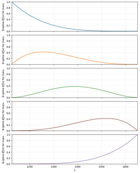
Figure 3. B-spline basis functions (of order 4) used to model the effect of vehicle mass. Each curve represents one basis function over the range of observed mass values; their weighted linear combination yields a smooth, non-linear approximation of the mass–energy relationship employed in the EES-based velocity estimation.

Figure 4 shows an analogous set of basis functions for the deformation coefficient $C_s$. The independent variable on the horizontal axis has been rescaled to the interval from 0 to 1, which simplifies both the numerical computations and the interpretation. The shapes of the functions $g$₁, …, $g$₅ are qualitatively consistent with the corresponding functions for mass. The function g₁ decreases from the value one at the starting point to zero close to the end of the interval, the function g₅ increases in the opposite direction, whereas g₂, g_3, and $g_4$ have bell shaped profiles with maxima appearing successively in more distant parts of the domain. As before, these functions are non-negative, have compact support and together they constitute a smooth partition of unity on the domain of the coefficient $C_s$.

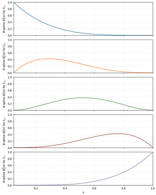
Figure 4. B-spline basis functions (of order 4) used to model the effect of vehicle deformation coefficient $C_s$. Each curve represents one basis function over the range of observed $C_s$ values.

From the modeling perspective both families of B-spline functions define flexible, yet well controlled functional bases used to approximate the unknown dependence of the response on mass and on the deformation coefficient. The model represents the effect of each of these variables as a linear combination of the corresponding basis functions, with parameters estimated from experimental data. The compact support of individual B-splines guarantees that the influence of the associated coefficients is local, which limits the risk of overfitting and facilitates interpretation of the results, whereas the smoothness of the basis ensures differentiability of the resulting functions and removes artificial oscillations. The use of separate but structurally identical bases for mass and for $C_s$ additionally allows a direct comparison of the sensitivity of the model response to changes in each of these variables.

In summary, Figure 3 and Figure 4 present the elementary components of the non-linear part of the model. The five B-spline functions for mass and the five functions for the deformation coefficient, defined on their respective intervals, span low-dimensional, smooth-function spaces in which the effects of both predictors are represented. The overlapping bell-shaped profiles of the interior functions, together with the monotonic boundary functions, provide numerical stability and a transparent interpretation of the relationships between the response of the system, mass, and the coefficient $C_s$.

The tensor products that correspond to the functions $h_k$, $k=1,\dots ,25$ can be seen in Figure 5. The Figure presents the two-dimensional basis functions obtained as tensor products of the one-dimensional B-spline functions describing the dependence on mass and on the deformation coefficient $C_s$. Each surface denoted by $h_k$, for $k$ from $1$ to $25$, is constructed as the product of an appropriate pair of functions $f_i$ and $g_j$ that were introduced earlier in Figure 3 and Figure 4. As a result, five times five equals twenty five, and local basis functions are obtained. They span a smooth function space of two variables and make it possible to represent a non-linear, non-stationary interaction between mass and the deformation coefficient $C_s$.

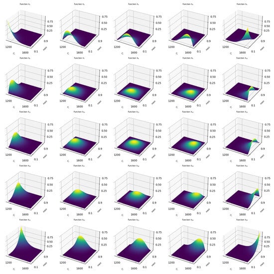
Figure 5. Tensor products of B-splines used for approximation (functions $h_k$).

In the upper left panel of Figure 5 one can observe the function h₁, which is the product of the boundary functions f₁ and g₁. Both of these functions take their largest values near the lower ends of their domains, that is, for the smallest values of mass and of C_s. Consequently, the surface h₁ attains its maximum in the corner corresponding to low mass and low deformation and then rapidly decays in the direction of growing arguments. From the interpretative point of view, h₁ represents a local component of the model that describes the behavior of the response only in this specific region of the parameter space and does not influence the result elsewhere.

In the remaining panels of the first row there are functions $h_2$, $h_3$, $h_4$, and $h_5$. In each case the factor related to mass is the same, namely f₁, whereas the factor associated with $C_s$ is changed successively from $g_2$ to $g_5$. The resulting surfaces share a similar profile in the mass direction, but their maxima move gradually toward larger values of $C_s$. Thus, the whole top row of Figure 5 corresponds to local components of the model associated with small values of mass and with a wide range of deformation levels, from low to high. An analogous interpretation holds for the last row, where the functions contain the factor $f_5$ and are therefore concentrated at the upper end of the mass range. In that case the maxima again move along the $C_s$ axis, but the support of the functions is restricted to the region of large mass.

The middle rows of the figure contain the functions $h_k$ that are obtained as products of the interior basis functions $f$₂, $f$₃, $f$₄ and $g$₂, $g$₃, $g$₄. Their profiles have the form of smooth hills located in different parts of the two-dimensional domain. The functions h₇ to h₉, which correspond to the products of f₂ with successive functions $g_j$, represent regions of low to medium mass combined with increasing values of $C_s$. The third row, containing functions with indices from 11 to 15, covers the central part of the domain with respect to both mass and deformation. These basis functions are particularly important when experimental observations are concentrated around intermediate values of the predictors, because they allow one to capture subtle changes of the response in the most typical range of parameters.

It is worth noting that each function $h_k$ is non-negative and has compact support, which means that it takes non-trivial values only in a limited region of the plane spanned by mass and $C_s$. In this way the tensor products preserve the key advantages of the one-dimensional B-spline bases. First, they provide local control over the shape of the estimated surface. A change in the coefficient associated with one basis function $t{h}_k$ affects the model only in the region where this function differs from zero. Second, the family $no\left\{h_k\right\}$ inherits the property of forming a smooth partition of unity. For any admissible pair of arguments, the sum of all basis functions is constant, which promotes numerical stability and facilitates interpretation of the estimated coefficients.

From the point of view of result analysis, it is important that the constructed system of tensor product basis functions makes it possible to describe in detail both the main effects and the interaction between mass and the deformation coefficient. If any model parameter attached to $h_k$ differs significantly from zero, this indicates that in the corresponding region of the two-dimensional parameter space the response exhibits a specific behavior that cannot be explained solely by additive one dimensional effects. In particular, a positive coefficient associated with a function localized in the corner of large mass and large $C_s$ points to an increase of the response in this area, whereas a negative coefficient would signal its decrease relative to what could be expected on the basis of a simple sum of the separate effects of mass and $C_s$.

Figure 5 also reveals the high regularity and symmetry of the constructed basis. The maxima of individual functions form an almost regular grid that covers the entire range of parameters. This guarantees a comparable ability to approximate the investigated phenomenon in all regions of the domain, rather than concentrating the flexibility of the model in only one part of the parameter space. In practice, the model can thus capture, with similar precision, for example an increased sensitivity of the response at low mass and medium deformation as well as non-linear effects that arise at high mass and low values of $C_s$.

In summary, the functions $h_k$ displayed in Figure 5 form a complete and well-conditioned basis of functions of two variables that forms the foundation of the non-linear part of the model. The tensor products of B-spline functions provide at the same time smoothness of the estimated surface, locality of the influence of individual coefficients, and a regular coverage of the entire parameter space. Such a construction allows for a transparent interpretation of the joint effect of mass and the coefficient $C_s$ on the response, and in particular facilitates the identification of those regions, where non-linear interactions between the two predictors are present.

2.4. Software

For the numerical analysis we utilized Python (ver. 3.10), along with the numpy (ver. 1.26.4) for array-oriented computations and model optimization, and scipy (ver. 1.15.3) for statistical tests. Visualization was conducted with matplotlib Python module (ver. 3.10.5).

3. Results

Let us begin with a plot depicting the weights that were used during the model training. The figure shows that velocities slightly above $13$ and just below $16\mathrm{m}/\mathrm{s}$ are the most crucial. The points with their weight above 0.5 can be considered quite typical. The ones between 0.3 and 0.4 can be perceived as moderately dependable, with some possible measurement error present. Points for which the weight drops below 0.1 are generally considered unreliable. This is shown in the following Figure 6.

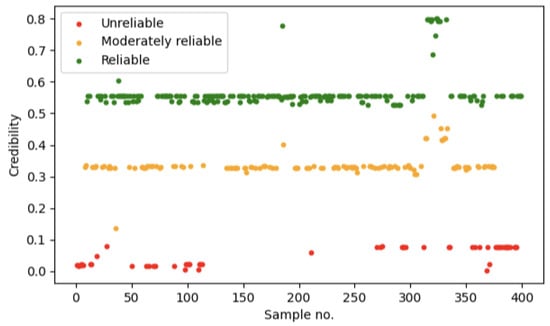
Figure 6. Weights/credibility of every observation. Green, orange, and red colors are used to distinguish reliable observations from unreliable ones.

The presented plot shows the distribution of weights assigned to individual observations used in the model training process. The horizontal axis represents successive observations corresponding to measured velocities, whereas the vertical axis shows the numerical values of the weights, which vary between 0 and 0.82. These weights are interpreted as a quantitative measure of the reliability of the data and of their importance for the estimation of the model parameters. In addition, each observation is marked with one of three colors, green, orange, or red, which qualitatively reflects the level of confidence in a given data point.

According to the accompanying description, observations corresponding to velocities slightly above $13 \mathrm{m}/\mathrm{s}$ and just below $16 \mathrm{m}/\mathrm{s}$ are of particular importance for the model. In this range the assigned weights attain the highest values, which means that these observations have the greatest influence on the fit of the model to the data. Observations with weights exceeding $0.5$ are treated as typical and highly reliable, and on the plot, they are represented mainly by green points concentrated in the upper part of the panel. Data with weights in the interval from 0.3 to 0.4 are regarded as moderately reliable, which suggests the presence of a non-negligible measurement noise, although these observations still provide useful statistical information. In contrast, observations with weights below 0.1, colored in red, should be considered as having low reliability, potentially affected by substantial measurement error or representing outliers.

Inspection of the spatial arrangement of the points reveals three characteristic levels of weights. The highest level is formed predominantly by green observations with weights around 0.55 and higher, which constitute the most numerous group, and indicate that the majority of the data is of generally good quality. Below this, one can identify a band of orange points with weights close to 0.3. Their number is smaller, but they are present across the entire range of the horizontal axis and therefore complement the most reliable part of the dataset. The lowest level corresponds to weight values close to zero, up to about 0.1, and contains a limited subset of the least reliable observations. This structure clearly shows that the dataset has been intentionally reweighted using several discrete levels of importance rather than through a completely continuous scheme.

The distribution of colors along the horizontal axis additionally reflects the variation in data quality across the velocity range. Green and orange observations occur throughout the analyzed domain, which indicates that in each segment there exist data points of at least moderate quality. Red points appear more frequently at the extremes of the range, both at the beginning and at the end of the axis. This pattern can be interpreted as increased uncertainty of measurements for very low or very high velocities, or as a consequence of a smaller number of experimental repetitions in those regions. As a result, the central part of the considered interval seems to be better represented and more trustworthy than its boundaries.

From a methodological perspective, the use of differentiated weights for the observations is a tool for increasing the robustness of the model with respect to noise and outliers. High weights assigned to observations regarded as typical ensure that these data dominate in the estimation of the parameters and in shaping the functional form that describes the investigated phenomenon. Observations with intermediate weights play a supporting role, allowing additional variability of the data to be captured while limiting their influence in the presence of stronger noise. Very low weights associated with red observations strongly reduce their contribution to the estimation, which prevents potential errors or extreme values from distorting the global fit of the model.

In summary, the analyzed plot provides a clear graphical representation of the weighting procedure applied in the study. It explicitly displays the hierarchy of reliability among individual observations and indicates which of them have been considered crucial for the training of the model and that have been treated with greater caution. This form of presentation facilitates the interpretation of subsequent modeling results, in particular by identifying those velocity ranges for which the model predictions can be regarded as most reliable and those regions where greater care is required when drawing substantive conclusions.

In the next step the parameters of the non-linear model were identified. For this purpose, the experimental data were substituted into the representation based on the tensor product B-spline basis functions (discussed in the previous Section), which led to a system of linear equations for the unknown coefficients α₁ to α₂₅. The system was solved via the least squares approach, so that the resulting set of coefficients minimizes the difference between the model predictions and the measured values. Solving this system to obtain coefficients ${\alpha }_k$, $k$ from 1 to 25 yields (10):

$$\begin{gathered} {\alpha }_1 = -644.967348, {\alpha }_2 = 766.121959, {\alpha }_3=-821.993890, {\alpha }_4 = 937.348043, {\alpha }_5 = -877.417981, \\ {\alpha }_6 = 789.037944, {\alpha }_7 = -855.774719, {\alpha }_8=936.563067, {\alpha }_9 = -991.676911, {\alpha }_{10} = 996.067530, \\ {\alpha }_{11} = -798.287292, {\alpha }_{12} = 885.389103, {\alpha }_{13}=-864.419542, {\alpha }_{14} = 997.692739, {\alpha }_{15} = -954.878218, \\ {\alpha }_{16} = 783.205530, {\alpha }_{17} = -766.462464, {\alpha }_{18}=767.388902, {\alpha }_{19} = -860.215549, {\alpha }_{20} = 905.916970, \\ {\alpha }_{21} = -633.912292, {\alpha }_{22} = 638.082846, {\alpha }_{23} = -579.225438, {\alpha }_{24} = 758.892584, {\alpha }_{25} = -763.166234. \end{gathered}$$

(10)

In Figure 7 the response surface obtained from the B-spline tensor product model is shown together with the experimental data points. The horizontal axes represent mass and the deformation coefficient C_s, whereas the vertical axis shows the corresponding values of V_t.

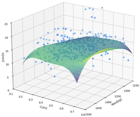
Figure 7. B-spline approximation of $V_t$, blue dots denote the observations from training part of the dataset.

The blue markers indicate individual observations, while the smooth-colored surface represents the non-linear prediction of the model. Visually, the surface follows the cloud of points quite closely. It bends in both directions and exhibits a gentle curvature that reflects the fact that the dependence of V_t on mass and C_s is not purely linear. In particular, for intermediate values of C_s the surface reaches a moderately elevated plateau, while toward the edges of the domain, especially for lower C_s and extreme masses, the predicted values of V_t decrease. This behavior suggests the presence of a non-linear interaction between the two predictors, which the tensor product of B-splines is able to capture.

Another important feature of Figure 7 is that the fitted surface smoothly interpolates between regions with different densities of data points. Where observations are more frequent, the surface visibly adapts to their local pattern, whereas in sparser regions it provides a reasonable extrapolation without unrealistic oscillations. The smooth shape of the surface indicates that the penalization and the choice of basis functions gave a stable estimator. The vertical separation between the data cloud and the surface is relatively small over most of the domain, which points to a satisfactory quality of fit, although some scatter of the points is clearly present and reflects the intrinsic variability of the measurements and the influence of unobserved factors.

For comparison, the linear least square approximation given by the following mapping (11):

$$\left(x, y\right)\to 1.943747 + 26.952362 · y + 0.007993 · x - 0.016550 · xy.$$

(11)

Figure 8 presents the corresponding approximation obtained from the linear least squares model defined by mapping (11). Here the surface is almost planar, with only a slight tilt introduced by the interaction term in the regression equation. In comparison with the B-spline surface, this plane is much less flexible. It cannot reproduce any local curvature in the relationship between $V_t$, mass and $C_s$. As a result, the linear surface intersects the point cloud in only a global, average sense. In some regions, especially where the B-spline surface bends upward or downward, the linear approximation either systematically overestimates or underestimates the observed values. This is visible in Figure 8 as larger vertical gaps between the plane and groups of points, particularly at combinations of mass and $C_s$, where the true response appears to deviate from a simple linear trend.

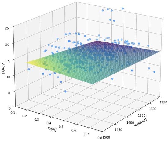
Figure 8. Linear approximation of $V_t$, blue dots denote the observations from training part of the dataset.

The comparison of the two figures clearly highlights the advantage of the non-linear B-spline approach for the present data set. The tensor product surface in Figure 7 adapts to the curved structure of the point cloud, so the fitted response increases or decreases at different rates depending on the region of the predictor space. This flexibility allows the model to represent, for example, a stronger influence of C_s for certain mass ranges and a weaker influence in others, which is consistent with the physical expectation that the effect of deformation may depend on the mass of the system. The linear model in Figure 8 imposes a much more restrictive structure. It assumes that the marginal effects of both mass and C_s are constant over the whole domain and that their interaction can be represented by a single bilinear term. Such a specification is too rigid to describe the subtle changes of slope that are visible in the experimental data.

From a modeling perspective the plots suggest that the B-spline tensor product model provides a more realistic description of the dependence of V_t on mass and C_s. It preserves smoothness and avoids abrupt changes, yet it allows for non-linear patterns and spatially varying interactions. The linear model is easier to interpret and requires fewer parameters, but at the cost of a poorer fit and a higher risk of systematic bias in regions where the true relationship departs from linearity. Therefore, for prediction purposes and for a detailed analysis of how mass and the deformation coefficient jointly influence V_t, the non-linear B-spline approximation shown in Figure 7 is clearly preferable to the simple plane shown in Figure 8.

The results presented in this chapter demonstrate that the quality and structure of the data have a decisive impact on the shape and performance of the proposed model. The initial analysis of observation weights shows that velocities slightly above 13 m/s and just below 16 m/s carry the highest credibility and therefore play the dominant role in parameter estimation. Observations with medium weights still contribute useful information but are treated with caution, while low weight observations are effectively down weighted, which limits the influence of outliers and measurement errors. This weighting scheme increases the robustness of the inference and clarifies in which regions of the velocity range the model predictions are most trustworthy.

Subsequent figures document the construction of the non-linear approximation based on B-spline functions. Univariate bases in mass and in the deformation coefficient $C_s$ provide smooth, locally supported components that span low dimensional function spaces. Their tensor products form a regular grid of two-dimensional basis functions $h_k$, which together describe both main effects and non-linear interactions between mass and $C_s$. The estimated coefficients attached to these functions define a flexible yet well-conditioned response surface that adapts to local patterns in the data while preserving smoothness and numerical stability.

The comparison of the B-spline tensor product model with the linear least squares approximation highlights the benefits of the non-linear approach. The B-spline surface follows the cloud of experimental points more closely, captures curvature and spatially varying interactions, and provides credible extrapolation in regions with fewer observations. The linear plane, although simple and easy to interpret, proves too restrictive and systematically misrepresents the response in areas where the true relationship departs from linearity. Overall, the analyses in this chapter indicate that the B-spline based model offers a more accurate and physically plausible description of the dependence of V_t on mass and $C_s$ than the corresponding linear alternative and therefore constitutes a more appropriate tool for both prediction and interpretation.

4. Discussion

To quantitatively compare the predictive performance of the linear and the B-spline based model, a single summary measure of prediction error was introduced. Since the observations in the data set carry different weights that reflect their credibility, and since the magnitude of the response varies across the domain, the error criterion had to take both of these aspects into account. For this reason, a weighted mean relative error was used, which expresses the absolute prediction error at each point in relation to the observed value and then aggregates these quantities with the same weights that were employed during model estimation. The weighted relative error was calculated according to the following Formula (12):

$$w_{r_{error}}:={\displaystyle \frac{{\sum }_{j=1}^N{w}_n\left|\frac{{B(x_n,y_n)-z}_n}{z_n}\right|}{{\sum }_{j=1}^N{w}_n}}$$

(12)

where $B$ denotes the B-spline approximating the data points. This weighted mean relative error is ≈5.20%. For comparison, the weighted mean relative error for the linear model is ≈5.47%.

Last but not least, in order to illustrate these numerical differences in a more direct way, 23 records were randomly selected from the test portion of the data set containing 338 observations. For this subset, a comparison of the predictions of the linear and non-linear models side by side was performed. The relevant results are reported in Table 2.

Table 2. A comparison of linear and B-spline approximations on the test set.

$\mathit{M}\mathit{a}\mathit{s}\mathit{s} \left[\mathbf{k}\mathbf{g}\right]$	${\mathit{C}}_{\mathit{s}} \left[\mathbf{m}\right]$	${\mathit{V}}_{\mathit{t}} [\mathbf{m}/\mathbf{s}]$	Linear Prediction $[\mathbf{m}/\mathbf{s}]$	B-Spline Prediction $[\mathbf{m}/\mathbf{s}]$	Linear Method Absolute Error $[\mathbf{m}/\mathbf{s}]$	B-Spline Method Absolute Error $[\mathbf{m}/\mathbf{s}]$	Linear Method Relative Error $\left[\mathit{\%}\right]$	B-Spline Method Relative Error $\left[\mathit{\%}\right]$
1300	0.533025	13.222222	15.232985	15.357379	2.010763	2.135157	15.2075	16.1482
1337	0.5894	15.611111	15.474367	15.557179	0.136744	0.053932	0.8759	0.3455
1358	0.6043	15.638889	15.504097	15.559296	0.134792	0.079593	0. 8619	0.5089
1439	0.43405	13.222222	14.8073	14.457246	1.585078	1.235024	0.11988	0.093405
1252	0.534	15.722222	15.27883	15.49253	0.443392	0.229692	0.028202	0.014609
1438	0.5805	15.777778	15.268387	15.329107	0.509391	0.448671	0.032285	0.028437
1335	0.4652	15.638889	14.874456	15.054556	0.764433	0.584333	0.04888	0.037364
1411	0.6209	13.111111	15.457442	15.489724	2.346331	2.378613	0.178957	0.18142
1465	0.6359	15.722222	15.374778	15.707607	0.347444	0.014615	0.022099	0.00093
1391	0.4235	13.194444	14.726963	14.64385	1.532519	1.449406	0.116149	0.10985
1308	0.4449	15.833333	14.758818	14.845378	1.074515	0.987955	0.067864	0.062397
1369	0.4667	15.75	14.890895	14.966149	0.859105	0.783851	0.054546	0.049768
1456	0.6305	16.138889	15.382135	15.650328	0.756754	0.488561	0.04689	0.030272
1379	0.4811	15.638889	14.953064	14.970964	0.685825	0.667925	0.043854	0.042709
1394	0.4677	15.722222	14.901506	14.808045	0.820716	0.914177	0.052201	0.058146
1382	0.581	15.527778	15.360822	15.397854	0.166956	0.129924	0.010752	0.008367
1453	0.3681	13.25	14.627001	14.190058	1.377001	0.940058	0.103925	0.070948
1419	0.4165	16.888889	14.730239	14.439901	2.15865	2.448988	0.127815	0.145006
1432	0.46958	13.388889	14.917221	14.643239	1.528332	1.25435	0.114149	0.093686
1368	0.1912	14.75	13.702551	13.936378	1.047449	0.813622	0.071013	0.055161
1353	0.3863	13.333333	14.51991	14.61641	1.186577	1.283077	0.088993	0.096231
1329	0.3433	15.552778	14.268328	14.277156	1.28445	1.275622	0.082587	0.082019
1379	0.3531	15.694444	14.424375	14.447877	1.270069	1.246567	0.080925	0.079427

Table 2 provides a pointwise comparison of the predictive performance of the linear model and the non-linear B-spline model on a randomly selected subset of 23 observations from the test set. For each record the table lists the input variables, that is, mass and the deformation coefficient $C_s$, the measured terminal velocity $V_t$, the corresponding predictions of both models, and the absolute and relative prediction errors. In this way the table complements the global error measures by showing how the two approaches behave across different regions of the predictor space.

Looking first at the absolute errors, one can see that in the majority of cases the B-spline approximation is more accurate. For 18 out of the 23 test points the absolute error of the B-spline model is smaller than the error of the linear model, while in five cases the linear model performs slightly better. The typical magnitude of the absolute error for both models lies between about 0.2 and 1.3 m/s. The mean absolute error over this subset is roughly 1.05 m/s for the linear model, compared with about 0.95 m/s for the B-spline model, which corresponds to an improvement of the order of several percent.

Several rows illustrate particularly large gains obtained with the non-linear model. For the observation with mass equal to 1465 kg and $C_s$ equal to 0.6359, both models predict a terminal velocity close to the measured value of $15.72 \mathrm{m}/\mathrm{s}$, but the linear model still exhibits an absolute error of about $0.35\mathrm{m}/\mathrm{s}$, whereas the B-spline model almost perfectly reproduces the measurement, with an error close to zero. A similar improvement is visible for mass 1456 kg and $C_s$ 0.6305, where the error decreases from approximately $0.76 \mathrm{m}/\mathrm{s}$ for the linear model to about $0.49 \mathrm{m}/\mathrm{s}$ for the B-spline model. In the case of mass 1453 kg and $C_s$ 0.3681, the absolute error drops from about $1.38 \mathrm{m}/\mathrm{s}$(linear model) to $0.94 \mathrm{m}/\mathrm{s}$ (nonlinear one), which is a substantial relative reduction. These examples indicate that the non-linear model is particularly effective in regions of larger mass, where the relationship between the predictors and $V_t$ appears to deviate more strongly from linearity.

There are, however, situations in which the linear model performs slightly better. For instance, for mass 1394 kg and $C_s$ 0.4677 the linear approximation yields an absolute error of about $0.82 \mathrm{m}/\mathrm{s}$, while the B-spline model produces an error of roughly 0.91 m/s. A similar pattern is observed for mass 1353 kg and $C_s$ 0.3863 and for mass 1419 kg with $C_s$ 0.4165, where the linear model provides somewhat smaller errors. In all these cases the differences remain moderate, which suggests that in parts of the domain where the true response is close to linear, the additional flexibility of the B-spline model does not necessarily translate into a sizeable gain in accuracy.

The relative errors of both models reported in Table 2, when interpreted in conjunction with the absolute errors, confirm these observations. Wherever the absolute error of the B-spline model is smaller, its relative error is reduced as well, indicating a better approximation of the local behavior of $V_t$. For example, at mass 1252 kg and $C_s$ 0.534, both models reproduce the measured velocity of 15.72 m/s quite well, but the relative error of the B-spline model is roughly half that of the linear model. In contrast, for mass 1300 kg and $C_s$ 0.533025, both models overestimate the true value of $13.22 \mathrm{m}/\mathrm{s}$ by more than $2 \mathrm{m}/\mathrm{s}$, and here the non-linear model performs slightly worse than the linear one. Such cases reflect local irregularities or higher noise levels in the data and point to regions where both modeling strategies struggle.

Overall, the detailed results in Table 2 show that the B-spline model provides a systematically more accurate description of the relationship between $V_t$, mass and $C_s$ on the test set, although the improvement is not uniform across all individual observations. The non-linear model brings the greatest benefit in those parts of the predictor space where the response surface is curved or where interaction effects are stronger, while in nearly linear regions the simpler linear model remains competitive. This nuanced picture is consistent with the visual comparison of the fitted surfaces and supports the conclusion that the B-spline approach offers a better compromise between flexibility and predictive accuracy for the data analyzed in this study.

Figure 9 provides a graphical summary of the pointwise errors of both models for the 23 test observations discussed in Table 2. The horizontal axis represents the sample index within the test subset, while the vertical axis shows the signed prediction error, that is the difference between the predicted and the observed value of $V_t$. The green horizontal line corresponds to zero error and therefore serves as a visual reference. Red squares denote the errors of the linear model and blue diamonds denote the errors of the B-spline model.

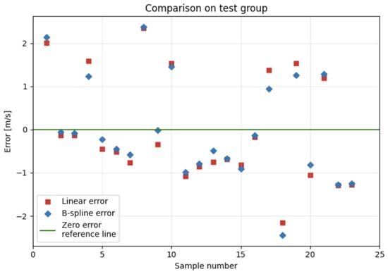
Figure 9. Plot depicting errors on the test set for each method (red for linear error, blue for B-spline error).

For most samples both markers lie on the same side of the zero line, which indicates that the two models tend to overestimate or underestimate the response in a similar way. However, the absolute distance from the zero line differs between the methods. In the majority of cases the blue diamonds are located closer to the reference line than the red squares, which means that the B-spline model yields smaller errors. This is especially visible for samples around indices 4, 9, 13, 17, and 20, where the non-linear approximation substantially reduces the magnitude of the error relative to the linear model. There are also a few samples, for example near indices 1, 15, 18, and 21, where the red marker is slightly closer to zero, showing that the linear model can be competitive or even marginally superior in some local situations.

The errors for both models do not exhibit any obvious systematic trend, which supports the assumption that the residuals are mainly driven by random variation rather than by a strong structural deficiency of the models. Nevertheless, the larger excursions from zero, such as those visible for the first and eighth sample, indicate regions of the predictor space where both models struggle and where the data may contain more noise or be less representative. Overall, the visual comparison in Figure 9 is consistent with the numerical results. It confirms that the B-spline model reduces the prediction error for most test observations and therefore provides a more accurate description of the relationship between $V_t$, mass and $C_s$ than the corresponding linear model.

In summary, the quantitative evaluation based on the weighted mean relative error shows that both models provide reasonably accurate predictions, with a slight but consistent advantage of the B-spline approach. The global error of about 5.20 percent for the non-linear model compared with 5.47 percent for the linear regression indicates that incorporating flexible spline bases yields a modest reduction in prediction error while still respecting the weighting scheme that reflects the credibility of individual observations. Interestingly, the normality testing for residuals shows that errors in B-spline approximation can be perceived as normal (p-value: 0.2327 for Shapiro test, test statistic: 0.94526). Unfortunately, the same cannot be said about the linear model (p-value: 0.0276, test statistic: 0.90186). Confidence intervals were obtained via non-parametric bootstrap resampling of crash cases. The linear model yields 95% bootstrap CI for absolute relative error equal to [5.88%, 7.03%] when tested on the entirety of test dataset with 1000 resamples. Analogously, 95% bootstrap CI was calculated for the non-linear approach: [5.19%, 6.32%]. This indicates better generalization with smaller—albeit only slightly—interval width (which may indicate improvement in overall robustness).

The detailed inspection of 23 randomly selected test cases confirms this global picture. In most rows of Table 2 the absolute and relative errors of the B-spline model are smaller than those of the linear model, especially in regions where the relationship between $V_t$, $mass,$ and $C_s$ is visibly non-linear. The linear model remains competitive in locally almost linear regions, but its errors increase in areas with stronger curvature or interaction effects. The error plot for the test subset reinforces these findings, showing that B-spline residuals usually lie closer to the zero-error line and do not exhibit systematic patterns across samples. Taking it all into consideration, the presented results indicate that the B-spline based model offers a better compromise between flexibility and predictive accuracy and therefore constitutes the preferred specification for describing the dependence of $V_t$ on mass and the deformation coefficient $C_s$.

From a statistical perspective, penalized B-splines reduce model misspecification bias relative to standard linear regression and allows for explicit management of the bias–variance trade-off through smoothing penalties [42]. This results in overall more stable velocity estimates, especially when deformation data are noisy or sparsely sampled. The B-spline tensor product model, combined with the probabilistic weighting of observations, yields a weighted mean relative error of approximately 5.2 percent. The corresponding linear model with probabilistic weights attains an error close to 5.5 percent. Although the numerical difference between these two values may appear modest at first glance, it is systematic and is observed both in global error indicators and in case-by-case comparisons on the test set, which indicates that the non-linear representation captures relevant features of the data that are inaccessible to purely linear approaches.

5. Conclusions

The authors have endeavored to further improve the method of pre-crash velocity determination within an Equivalent Energy Speed (EES) framework. The B-spline model does not replace the physical EES principle but instead capitalizes on top of it to provide a robust and physically plausible approximation of the deformation–energy relationship that underlies velocity estimation. As vehicle structural response to impact is continuous and inherently non-linear, global linear models are ineffective in capturing the stiffness characteristics of the vehicle. In continuity with earlier studies, in which various non-linear approaches were tested, the present work confirms that extending the traditional linear framework by means of flexible basis functions leads to a substantial gain in robustness, while maintaining high accuracy. In short,

• The B-spline tensor product model, combined with the probabilistic weighting of observations, was proposed to improve EES estimation by providing a robust and physically plausible non-linear approximation of the deformation–energy relationship.
• The need for flexible basis functions stems from the fact that global linear models are ineffective in capturing the stiffness characteristics of the vehicle, as its structural response to impact is continuous and inherently non-linear.
• The B-spline tensor product model with probabilistic weighting achieved a weighted mean relative error of approximately 5.2 percent, demonstrating a systematic advantage in accuracy and robustness over the corresponding linear model with probabilistic weights, which attained an error close to 5.5 percent.

When these results are compared with previously investigated approaches, the improvement becomes even more apparent. For the inverse system method, the weighted relative errors for the linear and non-linear variants were approximately 10.58 percent and 16.22 percent, respectively, while the Legendre polynomial approximation produced errors of about 6.74 percent for the linear model and 6.30 percent for the non-linear one. The current B-spline-based procedure clearly outperforms these earlier techniques, both in the linear and non-linear versions. This confirms the usefulness of the proposed weighting scheme, which incorporates information about the credibility of individual tests, and demonstrates that the B-spline tensor basis provides a convenient and powerful tool for approximating complex relationships between crash parameters and pre-impact velocity.

At the same time, the study highlights several limitations and directions for further development. The analysis has been carried out for the Compact vehicle class, which restricts the variability of structural and dynamic properties represented in the data set. A larger database encompassing a greater number of cases would allow for a more thorough validation of the method and would increase the reliability of the derived models. Additional information about vehicle characteristics, such as body structure details or energy absorption parameters, could also be incorporated as explanatory variables, potentially reducing the residual variability. Finally, extending the database toward higher and more diverse impact velocities would make it possible to verify the robustness of the B-spline approximation over a wider operating range. Despite these limitations, the present results indicate that the proposed probabilistic B-spline approach constitutes a promising and practically relevant step toward more accurate estimation of pre-crash velocity in real world accident reconstruction.

In further research the authors will verify the proposed method on a broader data set that includes other vehicle classes, more diverse crash configurations, and a wider range of impact velocities, and they will also consider more advanced weighting schemes based on formal uncertainty modeling, in order to further assess the universality and practical applicability of the B-spline-based EES approximation.

References

- Jankowski, K.P.; Gidlewski, M.; Jemioł, L. Comparative study of vehicle absorbed energy determination for road accident reconstruction. In Proceedings of the XVI EVU Annual Meeting, Kraków, Poland, 8–10 November 2007. [Google Scholar]
- Wąsik, M.; Skarka, W. Simulation of crash tests for electrically propelled flying exploratory autonomous robot. In Proceedings of the Transdisciplinary Engineering: Crossing Boundaries—Proceedings of the 23rd ISPE Inc. International Conference on Transdisciplinary Engineering, Curitiba, Brazil, 3–7 October 2016; IOS Press: Amsterdam, The Netherlands, 2016; pp. 3–7. [Google Scholar]
- Sharma, S.; Brophy, J.; Choi, E. An overview of NHTSA’s crash reconstruction software WinSMASH. In Proceedings of the 20th International Conference on the Enhanced Safety of Vehicles, Lyon, France, 18–21 June 2007; National Highway Traffic Safety Administration: Washington, DC, USA, 2007. [Google Scholar]
- Siddall, D.; Day, T. Updating the Vehicle Class Categories; SAE Technical Paper 960897; Society of Automotive Engineers: Warrendale, PA, USA, 1996. [Google Scholar] [CrossRef]
- Foret-Bruno, J.Y.; Trosseille, X.; Le Coz, J.Y.; Bendjellal, F.; Steyer, C.; Phalempin, T.; Villeforceix, D.; Dandres, P.; Got, C. Thoracic Injury Risk in Frontal Car Crashes with Occupant Restrained with Belt Load Limiter; SAE Technical Paper 983166; Society of Automotive Engineers: Warrendale, PA, USA, 1998. [Google Scholar] [CrossRef]
- Campbell, B.J. The traffic accident data project scale. In Proceedings of the Collision Investigation Methodology Symposium, Warrenton, VA, USA, 24–28 August 1969; pp. 675–681. [Google Scholar]
- Cromack, J.R.; Lee, S.N. Consistency Study for Vehicle Deformation Index; SAE Technical Paper 740299; Society of Automotive Engineers: Warrendale, PA, USA, 1974. [Google Scholar] [CrossRef]
- Hight, P.; Fugger, T., Jr.; Marcosky, J. Automobile Damage Scales and the Effect on Injury Analysis; SAE Technical Paper 920602; Society of Automotive Engineers: Warrendale, PA, USA, 1992. [Google Scholar] [CrossRef]
- Iraeus, J.; Lindquist, M. Pulse shape analysis and data reduction of real-life frontal crashes with modern passenger cars. Int. J. Crashworthiness 2015, 20, 535–546. [Google Scholar] [CrossRef]
- Wood, D.P.; Simms, C.K. Car size and injury risk: A model for injury risk in frontal collisions. Accid. Anal. Prev. 2002, 34, 93–99. [Google Scholar] [CrossRef] [PubMed]
- Geigl, B.C.; Hoschopf, H.; Steffan, H.; Moser, A. Reconstruction of occupant kinematics and kinetics for real-world accidents. Int. J. Crashworthiness 2003, 8, 17–27. [Google Scholar] [CrossRef]
- Vangi, D. Simplified method for evaluating energy loss in vehicle collisions. Accid. Anal. Prev. 2009, 41, 633–641. [Google Scholar] [CrossRef] [PubMed]
- Vangi, D.; Cialdai, C. Evaluation of energy loss in motorcycle-to-car collisions. Int. J. Crashworthiness 2014, 19, 361–370. [Google Scholar] [CrossRef]
- Faraj, R.; Holnicki-Szulc, J.; Knap, L.; Senko, J. Adaptive inertial shock-absorber. Smart Mater. Struct. 2016, 25, 035031. [Google Scholar] [CrossRef]
- Grolleau, V.; Galpin, B.; Penin, A.; Rio, G. Modelling the effect of forming history in impact simulations. Int. J. Crashworthiness 2008, 13, 363–373. [Google Scholar] [CrossRef]
- Wurong, W.; Sun, X.; Wei, X. Integration of forming effects into vehicle front rail crash simulation. Int. J. Crashworthiness 2016, 21, 9–21. [Google Scholar]
- Wach, W.; Gidlewski, M.; Prochowski, L. Modelling reliability of vehicle collision reconstruction based on the law of conservation of momentum and Burg equations. In Proceedings of the 20th International Scientific Conference TRANSPORT MEANS, Juodkrante, Lithuania, 5–7 October 2016; pp. 693–698. [Google Scholar]
- Żuchowski, A. The use of energy methods for calculation of vehicle impact velocity. Arch. Automot. Eng. 2015, 68, 85–111. [Google Scholar]
- Lindquist, M.; Hall, A.; Björnstig, U. Real world car crash investigations–A new approach. Int. J. Crashworthiness 2003, 8, 375–384. [Google Scholar] [CrossRef]
- McHenry, R. Computer Program for Reconstruction of Highway Accidents; SAE Technical Paper 730980; Society of Automotive Engineers: Warrendale, PA, USA, 1973. [Google Scholar] [CrossRef]
- Wach, W.; Unarski, J. Determination of Vehicle Velocities and Collision Location by Means of Monte Carlo Simulation Method; SAE Technical Paper 2006-01-0907; Society of Automotive Engineers: Warrendale, PA, USA, 2006. [Google Scholar] [CrossRef]
- Prochowski, L. The analysis of a car motion path after collision with a concrete barrier. Eksploat. Niezawodn.Maint. Reliab. 2011, 13, 71–80. [Google Scholar]
- Prochowski, L.; Żuchowski, A. Analysis of the influence of passenger position in a car on the risk of injuries during an accident. Eksploat. Niezawodn. Maint. Reliab. 2014, 16, 360–366. [Google Scholar]
- Gidlewski, M.; Prochowski, L. Analysis of motion of the body of a motor car hit on its side by another passenger car. IOP Conf. Ser. Mater. Sci. Eng. 2016, 148, 012039. [Google Scholar] [CrossRef]
- Kubiak, P. Work of non-elastic deformation against the deformation ratio of the subcompact car class using the variable correlation method. Forensic Sci. Int. 2018, 287, 47–53. [Google Scholar] [CrossRef]
- Kubiak, P.; Wozniak, M.; Karpushkin, V.; Jozwiak, P.; Ozuna, G.; Madziara, S.; Najbert, M.; Szosland, A. The method of determining velocity by measuring the vehicle-body deformation plane approximation method. In Proceedings of the International Conference on Engineering, London, UK, 1–3 July 2015; Springer: Singapore, 2016; pp. 43–57. [Google Scholar] [CrossRef]
- Brach, R.M.; Brach, R.M.; Mink, R.A. Nonlinear Optimization in Vehicular Crash Reconstruction. SAE Int. J. Transp. Saf. 2015, 3, 17–27. [Google Scholar] [CrossRef]
- Liu, Q.; Liu, J.; Wu, X.; Han, X.; Cao, L.; Guan, F. An inverse reconstruction approach considering uncertainty and correlation for vehicle-vehicle collision accidents. Struct. Multidiscip. Optim. 2019, 60, 681–698. [Google Scholar] [CrossRef]
- Wang, X.; Peng, Y.; Yu, W.; Yuan, Q.; Wang, H.; Zheng, M.; Yu, H. Uncertain inverse traffic accident reconstruction by combining the modified arbitrary orthogonal polynomial expansion and novel optimization technique. Forensic Sci. Int. 2022, 333, 111213. [Google Scholar] [CrossRef] [PubMed]
- Riviere, C.; Lauret, P.; Manicom Ramsamy, J.F.; Page, Y. A Bayesian Neural Network approach to estimating the Energy Equivalent Speed. Accid. Anal. Prev. 2006, 38, 248–259. [Google Scholar] [CrossRef] [PubMed]
- Moravcová, P.; Bucsuházy, K.; Zůvala, R.; Semela, M.; Bradáč, A. What should I use to calculate vehicle EES? PLoS ONE 2024, 19, e0297940. [Google Scholar] [CrossRef]
- Mackay, G.M.; Hill, J.; Parkin, S.; Munns, J.A.R. Restrained occupants on the nonstruck side in lateral collisions. Accid. Anal. Prev. 1993, 25, 147–152. [Google Scholar] [CrossRef]
- McHenry, B. The algorithms of CRASH. 2001. Available online: https://www.researchgate.net/publication/237300782_THE_ALGORITHMS_OF_CRASH (accessed on 24 December 2025).
- Nelson, W.D. The History and Evolution of the Collision Deformation Classification; SAE Technical Paper 810213; Society of Automotive Engineers: Warrendale, PA, USA, 1981. [Google Scholar] [CrossRef]
- Neptune, J.E. Crush Stiffness Coefficients, Restitution Constants, and a Revision of CRASH3 & SMAC; SAE Technical Paper 980029; Society of Automotive Engineers: Warrendale, PA, USA, 1998. [Google Scholar] [CrossRef]
- Prochowski, L.; Kochanek, H.; Gidlewski, M.; Pusty, T. Analysis of seasonal and regional variations in accident hazard in Poland. WIT Trans. Built Environ. 2017, 176, 441–452. [Google Scholar]
- Bayarri, M.J.; Berger, J.O.; Kennedy, M.C.; Kottas, A.; Paulo, R.; Sacks, J.; Cafeo, J.A.; Lin, C.-H.; Tu, J. Predicting Vehicle Crashworthiness: Validation of Computer Models for Functional and Hierarchical Data. J. Am. Stat. Assoc. 2009, 104, 929–943. [Google Scholar] [CrossRef]
- Turoboś, F.; Koneczny, P.; Stajuda, Ł.; Levchenko, D.; Siczek, K.; Kubiak, P.; Mrowicki, A.; Madziara, S. Innovative precrash velocity calculation for forward-facing collisions using Gaussian process regression and modern vehicle data. In Proceedings of Automotive Safety 2024: Proceedings of the 14th International Science and Technical Conference Automotive Safety, Sandomierz, Poland, 24–26 April 2024; CRC Press: Boca Raton, FL, USA, 2025. [Google Scholar]
- Mrowicki, A.; Krukowski, M.; Turoboś, F.; Jaśkiewicz, M.; Radkowski, S.; Kubiak, P. Determining vehicle pre-crash speed in frontal barrier crashes using genetic algorithm model adjustment techniques for intermediate car class. Int. J. Crashworthiness 2021, 27, 1009–1016. [Google Scholar] [CrossRef]
- Mrowicki, A.; Krukowski, M.; Turoboś, F.; Kubiak, P. Determining vehicle pre-crash speed in frontal barrier crashes using artificial neural network for intermediate car class. Forensic Sci. Int. 2020, 308, 110179. [Google Scholar] [CrossRef]
- De Boor, C. Practical Guide to Splines: With 32 Figures; Springer: New York, NY, USA, 2001. [Google Scholar]
- Korsun, O.N.; Goro, S.; Om, M.H. A comparison between filtering approach and spline approximation method in smoothing flight data. Aerosp. Syst. 2023, 6, 473–480. [Google Scholar] [CrossRef]
Disclaimer/Publisher’s Note: The statements, opinions and data contained in all publications are solely those of the individual author(s) and contributor(s) and not of MDPI and/or the editor(s). MDPI and/or the editor(s) disclaim responsibility for any injury to people or property resulting from any ideas, methods, instructions or products referred to in the content. |
© 2025 by the authors. Licensee MDPI, Basel, Switzerland. This article is an open access article distributed under the terms and conditions of the Creative Commons Attribution (CC BY) license.