Training-Free and Environment-Robust Human Motion Segmentation with Commercial WiFi Device: An Image Perspective

Abstract

WiFi sensing relies on capturing channel state information (CSI) fluctuations induced by human activities. Accurate motion segmentation is crucial for applications ranging from intrusion detection to activity recognition. However, prevailing methods based on variance, correlation coefficients, or deep learning are often constrained by complex threshold-setting procedures and dependence on high-quality sample data. To address these limitations, this paper proposes a training-free and environment-independent motion segmentation system using commercial WiFi devices from an image-processing perspective. The system employs a novel quasi-envelope to characterize CSI fluctuations and an iterative segmentation algorithm based on an improved Otsu thresholding method. Furthermore, a dedicated motion detection algorithm, leveraging the grayscale distribution of variance images, provides a precise termination criterion for the iterative process. Real-world experiments demonstrate that our system achieves an E-FPR of 0.33% and an E-FNR of 0.20% in counting motion events, with average temporal errors of 0.26 s and 0.29 s in locating the start and end points of human activity, respectively, confirming its effectiveness and robustness.

1. Introduction

Intelligent sensing of human behavior in target spaces plays a pivotal role in smart cities, medical monitoring, human-computer interaction, and other fields. Compared with traditional video-based and sensor-based methods, utilizing ubiquitous WiFi signals for Human Motion Sensing (HMS) has garnered significant interest due to its non-invasiveness, wide coverage, strong adaptability, and low cost.

In various WiFi-based HMS technologies, the extraction of human motion intervals not only enables specific goals such as intrusion monitoring and energy management, but also serves as a cornerstone of advanced applications including indoor localization, health care, and activity recognition. The theoretical basis of WiFi-based human motion segmentation is that human body movement alters the channel properties of the communication link, which can be characterized by Channel State Information (CSI). Typically, the collected CSI in a static environment remains stable, but the presence of human movement disrupts this stability. Therefore, the states of human can be distinguished by developing appropriate metrics to quantify the CSI fluctuations.

In previous works, variance and the correlation coefficient are the most commonly used metrics. However, the variance-based method requires additional static data for threshold determination, while the correlation-based method faces challenges in clear distinguishing between static and dynamic states. Researchers have also explored deep learning methods for motion segmentation. However, CSI is highly environment-dependent, and its collection process is time-consuming and labor-intensive. These factors limit the application of learning-based methods.

To address the above issues, this paper proposes a training-free and environment-robust human motion segmentation method using commercial WiFi devices. By treating CSI data as an image rather than independent time series, we introduce a quasi-envelope to represent motion-induced fluctuations, thereby significantly enhancing the homogeneity of motion regions in the CSI image. In order to improve segmentation efficiency, we design an improved Otsu threshold calculation method, which is better meet practical segmentation needs. Furthermore, we propose an iterative segmentation algorithm to handle the distinct fluctuations caused by different types of human motion. Additionally, we introduce a novel human motion detection method, which provides a reliable criterion for terminating the iterative segmentation process. Experimental results demonstrate that the proposed method achieves accurate and robust human motion segmentation across different indoor scenarios without relying on learning models.

Generally, the main contributions of this paper can be summarized as follows:

• A quasi-envelope of CSI variance image is carefully used to represent the fluctuations caused by human motion, which effectively resolves the issue of motion fragmentation.
• From an image-processing perspective, we design a training-free and environment-adaptive human motion detection algorithm, and we calculate the key parameters based on the grayscale distributions of CSI image.
• An improved iterative segmentation algorithm is proposed to overcome the variations in CSI fluctuations caused by varying motion intensities, and extensive experimental results confirm its accuracy and robustness.

The rest of this paper is organized as follows. First, some related works on WiFi-based HMS are introduced in Section 2. Then, basic knowledge about CSI is explained in Section 3. In Section 4, the iterative human motion segmentation algorithm is discussed in detail, and in Section 5, the experiment results of the proposed method are described. Finally, we summarize the work done in Section 6. To enhance the readability of technical terms, the following Table 1 lists the main abbreviations used in this paper with their full names.

Table 1. Comparison of explanations of terms for the core abbreviations in this study.

Abbreviation	Full Title
HMS	Human Motion Sensing
CSI	Channel State Information
CNN	Convolutional Neural Network
MIMO	Multiple Input Multiple Outputs
OFDM	Orthogonal Frequency Division Multiplexing
SRG	Seeded Region Growing
CDF	Cumulative Distribution Function
E-FPR	Event-level False Positive Rate
E-PNR	Event-level False Negative Rate
MSSE	Motion Start-point Segmentation Error
MESE	Motion End-point Segmentation Error

2. Related Works

HMS using WiFi has drawn the attention of numerous researchers since work [1] released the open-source firmware that can capture the CSI from commercial network cards. A comprehensive literature search was performed across four major academic databases: Web of Science, IEEE Xplore, ACM Digital Library, and Google Scholar. Systematic retrieval was conducted using Boolean queries with the keywords WiFi and human motion for publications since 2010. Then, key publications were selected for in-depth analysis based on their representativeness, impact, and methodological relevance.

2.1. Human Motion Presence Detection

Simply detecting the presence of human movement is adequate for specific WiFi-based sensing requirements, such as intrusion detection and building energy management. Consequently, some studies have been devoted to human motion detection algorithms using CSI.

Volatility difference is the most evident and commonly used criterion for determining the presence of human movements. Bfp [2] constructs an offline database with the probability distribution histogram of static variance, and it adopts an Earth Mover’s Distance (EMD) algorithm to compare the similarity of the fingerprint and calculated variance. Ar-Alarm [3] constructed a robust human motion indicator using the standard deviation of the phase difference, and it removed the false intrusion alarm by magnitude-based filter. Moreover, the system can accommodate the environment change with the help of static profile updating mechanism. Similarly, ref. [4] also used the variance of phase difference for intrusion detection and calculated Effective Interference Height (EIH) to distinguish the movement of humans and pets.

Variations in temporal and spatial correlation are also frequently used to capture human movement. Ref. [5] proposed a correlation-based scheme for the detection of moving humans with the help of Support Vector Machine (SVM). WiSH [6] selected the cross-correlation in both time and frequency domains to detect human motion. Benefiting from the deployment of tiny WiFi nodes, the system was energy efficient compared with others. Ref. [7] proposed a link pair selection method in order to improve the signal quality and implemented intrusion detection, similar to ref. [5]. Ref. [8] verified the human motion detection bound based on the intrusion-distributed non-line-of-sight channel model, which provides a valuable reference for WiFi-based security system design.

Additionally, some works utilize machine learning or deep learning models to solve human motion detection problems [9]. Ref. [10] employed ESP32 to collect both Received Signal Strength Indicator (RSSI) and CSI data and extracted seven specific features for training ensemble machine learning models, which achieved an accuracy of up to 99.4% in classifying human motion in three different rooms. Ref. [11] compared the system performance of 31 machine learning algorithms using the statistics of CSI amplitude. Ref. [12] computed the Autocorrelation Function (ACF) of CSI and trained a neural network to learn patterns associated with human presence. In order to reduce false alarms and missed detections, a sliding window median filter was adopted to smooths the output. LowDetrack [13] utilized Compressed Sensing (CS) to supplement missing data at ultralow packet rates with WiFi and analyzed multiple features of CSI including variance, correlation matrices, and Doppler Frequency Shift (DFS) to determine the presence of moving and stationary human.

2.2. Human Motion Interval Segmentation

In advanced applications such as activity recognition and physiological parameter monitoring, it is often necessary to accurately determine the start and end points of human movement, making human motion intervals segmentation crucial for the system performance.

The most common activity segmentation method used in WiFi sensing is the threshold-based method. MoSense [14] designed a distance-based mechanism to select the subcarriers with richer environment information and employed the variance of phase difference to segment human motion, which obtained ideal performance in single motion and motion sequence cases. Moreover, it depicted a specifical silence analysis model aiming at the alignment problem in different static states. MoSeFi [15] delved into the properties of Möbius transformation and found that the real and imaginary parts of CSI ratio are complementary in shape. To this end, the authors integrated the variance sum of two parts as a new motion indicator, which greatly solves the problem of motion fragmentation and reduces the segmented motion duration error. LightSeg [16] considers the granularity of the activity and detects the end of a segment first using a threshold as 4% of the maximum value of the target activity variance, then decides the appropriate threshold based on the linear traversal of the current CSI stream.

Meanwhile, recent studies have also formulated the motion segmentation problem as a classification task, leveraging powerful deep learning methods to overcome challenges such as threshold setting and environmental interference [17]. DeepSeg [18] divided the continuous CSI streams into equal bins and adopted a Convolutional Neural Network (CNN) architecture to classify four states, including static-state, start-state, motion-state, and end-state. Then, it identified the start and end positions based on these state labels. Furthermore, it proposed a feedback mechanism between the segmentation and recognition models, which enhanced the overall system performance. Ref. [19] used the phase of CSI ratio as a feature and proposed a CNN based method for segmentation and identification of Parkinson′s hand tremor, and the results showed that feature enhancement was another means to improve system performance. SEGALL [20] proposed a novel signal-independent segmentation architecture that leverages a hybrid deep learning model combining Transformer and Long Short-Term Memory (LSTM) layers to address the challenge of segmenting continuous wireless sensing data under interference. Specifically, it reformulated segmentation as a binary classification problem rather than regression, labeling target activity periods as 1 and interference as 0 to mitigate label imbalance.

Despite notable advancements in WiFi-based human motion sensing, certain limitations persist. While threshold-based approaches are efficient, they are limited by the dependence on prior static data collection and poor adaptive capability. Although learning-based methods have demonstrated excellent performance, they require extensive annotated datasets for training. Therefore, developing a training-free and efficient method for motion monitoring and segmentation is of significant practical importance.

3. Preliminaries

3.1. About CSI

In wireless communication, the Channel Frequency Response (CFR) is used to describe the multipath propagation of the wireless signal, which is the Fourier transform of the Channel Impulse Response (CIR). CSI is the sampled version of CFR, which can be expressed as

$$H\left(f,t\right)={\sum }_l^L{a}_l\left(t\right)exp\left(-i2\pi f{\tau }_l\left(t\right)\right)$$

(1)

where $a_l\left(t\right)$ and ${\tau }_l\left(t\right)$ are the complex attenuation and propagation delay of the $l_{th}$ path, respectively, f is the subcarrier frequency, and L is the total number of paths. When the object moves in the wireless channel, the amplitude $\left|H\left(f,t\right)\right|$ and phase $\angle H\left(f,t\right)$ of the CSI will be modulated by environmental changes, thus endowing the CSI with the ability to perceive the environment. Suppose that at time t, the length changes of the $l_{th}$ path caused by the movement of the object is $d_l\left(t\right)$. Then, the propagation delay can be calculated as ${\tau }_l\left(t\right)=d_l\left(t\right)/c=d_l\left(t\right)/f\lambda$, where c is the speed of light. Thus, the phase shift $exp\left(-i2\pi f{\tau }_l\left(t\right)\right)$ can be written as $exp\left(-i2\pi d_l\left(t\right)/\lambda \right)$.

According to previous work [21], signal propagation paths can be divided into static and dynamic paths. Specifically, the static path includes the line-of-sight path and multiple reflection paths of fixed objects, while the dynamic path refers to the reflection paths whose length changes with the movement of the target. In most cases, we can assume that there is only one dominant reflection path. Thus, CSI can be expressed as

$$\begin{array}{cc}\hfill H\left(f,t\right)& =H_s\left(f,t\right)+H_d\left(f,t\right)\hfill \\ \hfill & =H_s\left(f,t\right)+a\left(t\right)exp\left(-i2\pi d\left(t\right)/\lambda \right)\hfill \end{array}$$

(2)

where $H_s\left(f,t\right)$ is the static component, and $a\left(t\right)$ and $d\left(t\right)$ are the complex attenuation and the change in path length of the dynamic component $H_d\left(f,t\right)$, respectively. From Equation (2), we can see that when the dynamic path changes, $H_d\left(f,t\right)$ rotates around $H_s\left(f,t\right)$ on the complex plane.

The collected CSI data are mainly affected by two factors [22]: (1) the amplitude noise $\Delta agc$ caused by the uncertain state of the auto-gained circuit and (2) the phase noise ${\theta }_{offset}$ caused by the time asynchronism of the transceivers. Thus, the raw CSI can be further expressed as follows:

$$\widehat{H}\left(f,t\right)=\Delta agc·exp\left(-i2\pi {\theta }_{offset}\right)·H\left(f,t\right)$$

(3)

Due to amplitude and phase noise, the collected CSI is distributed in a ring on the complex plane, as shown in Figure 1a. As a result, its amplitude fluctuates in a sinusoidal shape in the dynamic state while remaining stable in the static state, but the phase constantly changes randomly.

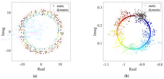
Figure 1. Distribution on the complex plane. (a) CSI. (b) CSI ratio.

3.2. Derived CSI Ratio

In a modern WiFi system, a wireless channel using Multiple Input Multiple Outputs (MIMO) is divided into subcarriers by Orthogonal Frequency Division Multiplexing (OFDM). For a MIMO-OFDM WiFi channel with M transmit antennas, N receive antennas, and K subcarriers, the CSI is a three-dimensional matrix $H\in {\mathbb{C}}^{N\times M\times K}$ [23]. Therefore, the whole CSI matrix provides us with more useful information in different domains, including time, frequency, and space. This allows us to construct new features for environmental perception.

Since commercial WiFi network cards use the same radio frequency chains and clock between different antennas, the amplitude noise $\Delta agc$ and phase offset ${\theta }_{offset}$ of each antenna are almost the same. Thus, if we calculate the quotient between the CSI of two antenna pairs, the above amplitude and phase noise is automatically removed. In general, the calculated result is referred to as the CSI ratio, which can be expressed as follows:

$$H_{CSI-ratio}={\displaystyle \frac{H_1\left(f,t\right)}{H_2\left(f,t\right)}}={\displaystyle \frac{H_{s,1}+A_{1}exp\left(-i2\pi d_1\left(t\right)/\lambda \right)}{H_{s,2}+A_{2}exp\left(-i2\pi d_2\left(t\right)/\lambda \right)}}$$

(4)

where $H_{s,[1,2]}$, $A_{[1,2]}$, and $d_{[1,2]}\left(t\right)$ denote the static component, the complex attenuation, and the dynamic path length of antennas 1 and 2, respectively.

Meanwhile, the difference in the reflection path between two approaching antennas can be seen as a constant when the target moves a short distance. If we assume $d_2\left(t\right)=d_1\left(t\right)+\Delta d$ in a short time period, then Equation (4) can be deformed as follows:

$$H_{CSI-ratio}={\displaystyle \frac{A_{1}exp\left(-i2\pi d_1\left(t\right)/\lambda \right)+H_{s,1}}{A_{2}exp\left(-i2\pi \Delta d\right)exp\left(-i2\pi d_1\left(t\right)/\lambda \right)+H_{s,2}}}$$

(5)

Therefore, the CSI ratio can be regarded as the Möbius transformation of $exp\left(-i2\pi d_1\left(t\right)/\lambda \right)$. As shown in Figure 1b, the distribution of the CSI ratio is concentrated around one point in the static state due to the zero dynamic component. When the dynamic path length changes by one wavelength, the trajectory of $exp\left(-i2\pi d_1\left(t\right)/\lambda \right)$ is a complete circle on the complex plane. Based on the conformality of the Möbius transformation, the trajectory of the CSI ratio is also a circle at this time.

Compared with the raw CSI, the derived CSI ratio has a higher Signal-to-Noise Ratio (SNR). It can be seen from Equation (4) that the amplitude noise ${\Delta }_{agc}$ and phase noise ${\theta }_{offset}$ are effectively eliminated based on the division operation. As a result, CSI ratio provides more usable information for WiFi sensing, including amplitude, phase and distance on the complex plane. They are all stable in a static environment, but they fluctuate in a dynamic environment. Therefore, the derived CSI ratio is increasingly used in WiFi perception instead of raw CSI.

3.3. CSI Image Perspective: Opportunities and Challenges

As described in Section 3.2, due to the use of OFDM and MIMO technology, the CSI data consist of multiple time series. When consolidated into a unified structure, these time series yield a $K\times T$ image. Owing to the complementary effect of CSI series, the CSI image effectively mitigates quality degradation caused by selective fading, thereby reducing the dependence on subcarrier selection. Therefore, treating CSI as an image rather than a set of independent time series allows us to leverage image processing techniques to address challenges in WiFi sensing.

Figure 2 presents a normalized CSI ratio amplitude image that containing two motion intervals. It can be seen that the fluctuations induced by human motion exceed those caused by background noise. Figure 3 further shows the variance image depicting the amplitude variations. It can be observed that the variance values of the static intervals are predominantly clustered near zero. In contrast, motion-induced fluctuations result in larger variance values in the dynamic counterparts.

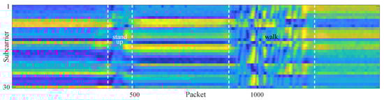
Figure 2. Amplitude of CSI ratio containing two motion intervals.

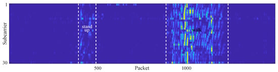
Figure 3. Variance of CSI ratio containing two motion intervals.

Unfortunately, traditional image segmentation algorithms based on grayscale distribution or clustering struggle to accurately segment motion regions. For instance, Figure 4a demonstrates the result obtained using the classic Otsu algorithm, where the segmentation accuracy is considerably poor. Due to uncertain degradation of subcarrier quality and the inevitable presence of peaks and troughs in amplitude series, the variance values of motion regions are distributed over a wide range, leading to an overlap with those in static regions. Thus, a considerable portion of pixels within the walking region are misclassified as static, which results in fragmented and discontinuous segmentation result. In addition, owing to variance differences induced by motion intensity, most pixels of the standing-up motion region are incorrectly classified as static, leading to a severe under-segmentation issue.

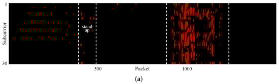
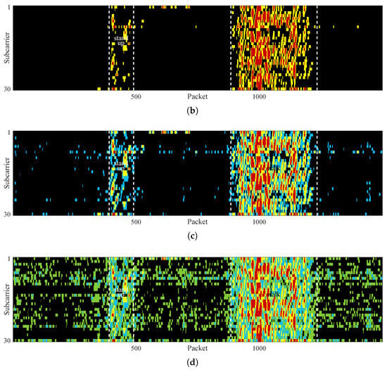
Figure 4. Segmentation results of (a) the first iteration, (b) the second iteration, (c) the third iteration, and (d) the fourth iteration.

Intuitively, re-segmenting pixels that are already classified as static could enhance segmentation performance [24]. Figure 4b–d confirm the above conjecture, where the dynamic pixels identified in each segmentation iteration are highlighted with different colors. It can be seen that more motion-region pixels are correctly detected as the iteration round increases, e.g., the integrity of the dynamic region in Figure 4b is significantly better than that in Figure 4a. However, a rise in iteration count also leads to more static pixels being misclassified as dynamic, as shown in Figure 4c,d. Furthermore, it can be seen that the spatial distribution of dynamic pixels extracted in each iteration exhibits irregularity, which is an inevitable consequence of the wide grayscale distribution of motion intervals. The above analysis indicates that treating CSI data as an image provides richer information, enabling the application of image processing methods to motion segmentation. Nevertheless, this approach still faces two major challenges: (1) how to enhance the grayscale homogeneity of motion regions and strengthen their distinction from static regions, thereby boosting segmentation effectiveness; (2) how to define a stopping criterion for the iterative segmentation process to handle fluctuations in CSI caused by different motions, so as to improve segmentation accuracy.

4. Method

4.1. Data Preprocessing

Denoise. Capitalizing on its superior noise-attenuation properties, the CSI ratio is employed for human motion segmentation rather than native CSI. To further suppress environmental noise interference, CSI ratio data are denoised using a Savitzky–Golay (SG) filter. The SG filter applies linear least squares fitting to sequential subsets of adjacent data points through low-degree polynomial approximation, effectively preserving signal peak morphology and spectral characteristics. The window size and polynomial order are experimentally set to 11 and 2, respectively.

Subcarrier Screening. Due to the influence of frequency selective fading, the subcarrier is affected differently by the environment. To balance static stability and dynamic sensitivity, a lightweight subcarrier selection method is adopted. Specifically, each CSI ratio series is divided into segments of equal length, and the variance of each segment is calculated. Subsequently, the sum of variances corresponding to each subcarrier is tallied, and the subcarriers with median sum values are selected for human motion sensing. Since the number of subcarriers is closely related to the quality of motion segmentation, this issue will be discussed in detail in Section 5.4.5.

4.2. Homogeneity Enhancement Based on Quasi-Envelope

To enhance clarity and conciseness, we utilize CSI data comprising a single dynamic interval to demonstrate quasi-envelope computation and the improved Otsu algorithm. It should be noted that the underlying principles and outcomes remain consistent for scenarios involving multiple motions.

4.2.1. Rethinking of Raw Variance

Figure 5 presents a variance series of the CSI ratio amplitude using orange line. Since the actual static CSI ratio is not a fixed value but fluctuates within a small range due to the environment and hardware noise, the variance values of static intervals fluctuate in a small range around zero rather than being strictly zero. For the dynamic interval, the sharp changes in CSI ratio cause the calculated variance to fluctuate within a wide range. Specifically, the variance values corresponding to the approximately linear part of the CSI series are much larger than those in the static state, while the variance values calculated from the peaks and troughs are relatively small, even close to those of static state. The variance values at the remaining positions are between the above two. Furthermore, when environmentally induced degradation of the subcarrier quality occurs, it also causes a significant reduction in the level of fluctuations arising from human motion.

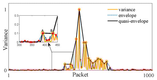
Figure 5. Illustration of quasi-envelope calculation.

Since the variance values of the dynamic region are distributed within a large range and overlap with those of the static region, the histogram of the original variance image is unimodal. On the one hand, the unimodal histogram prevents the Otsu algorithm from obtaining the correct segmentation threshold. On the other hand, the overlap of variance values makes it impossible to obtain a complete motion interval when using a single fixed threshold.

Therefore, the raw variance image is not an optimal choice for motion segmentation, and the excessive variations in variance within dynamic intervals account for the poor segmentation quality.

4.2.2. About Envelope

In physics and engineering, the envelope of an oscillating signal is defined as a smooth curve outlining the extrema of the signal, which is widely used in mechanical fault diagnosis and acoustic signal processing. The envelope can effectively remove the severe fluctuations while maintaining the whole characteristics of the original signal.

Typically, the envelope can be divided into upper and lower envelopes. For a piece of variance series, the upper and lower envelopes of the static interval are very close due to the small fluctuations, while the values of the upper envelope are usually much larger than those of the lower envelope in the dynamic interval. Obviously, the upper envelope provides a clearer distinction between the static and dynamic intervals; therefore, the following discussion is all about the upper envelope.

In general, the envelope can be calculated based on Hilbert Transformation (HT), moving Root Mean Square (RMS), and local peaks. In comparison, the calculation of peak is simple and flexible, and it is not affected by the window length. Thus, a peak-based method is selected for envelope calculation in this paper. Typically, obtaining the envelope from peaks usually involves two steps: first, finding the local peaks whose heights are greater than those of the two neighboring samples, and then interpolating the extreme points with an appropriate method.

For a given time series $x\left[n\right]$, a peak is defined as a point satisfying $x\left[n\right]\ge x\left[n-1\right]$ and $x\left[n\right]\ge x\left[n+1\right]$. By performing linear interpolation between two adjacent peaks, the envelope segment between them can be expressed as follows:

$$E\left[n\right]=x\left[n_i\right]+{\displaystyle \frac{x\left[n_{i+1}\right]-x\left[n_i\right]}{n_{i+1}-n_i}}(n-n_i),n_i\le n\le n_{i+1}$$

(6)

Since the local oscillations between adjacent peaks are eliminated, the resulting envelope exhibits greater smoothness than the original series.

Figure 5 shows an example of envelope calculation based on local peaks. Here, all extremes of the variance series are highlighted with red asterisks, and the envelope obtained through linear interpolation is plotted with a blue dashed line. It can be seen that the values of the envelope series are still small and stable in the static intervals, which is consistent with the original variance series. For the dynamic interval, since the troughs of the original variance sequence are mapped to relatively high values, the variation range of the envelope is effectively compressed into a smaller one, which makes the envelope values of dynamic interval almost all larger than those of the static intervals. Given that excessive variance fluctuations cause motion fragmentation and threshold problems, the envelope is well-suited to mitigate these issues.

4.2.3. Calculation of Quasi-Envelope

In the above operation, all local peaks participate in the calculation of envelope, resulting in a narrower distribution range within the motion interval. However, it can be seen that the heights of some peaks within the dynamic interval are still similar to those of the static intervals. The local magnified views in Figure 5 allows for more detailed observation of the effects of these factors on envelope computation. Since the values of peaks C and D are comparable to those of static state, their inclusion increases envelope fluctuations within the motion interval. Therefore, a strategy that selects only prominent peaks like A and B for envelope construction significantly enhances the homogeneity of dynamic intervals. Here, we refer to the indistinct peaks such as C and D as bad peaks.

Visually, a bad peak is either a subsidiary peak of a higher peak or an obscure independent one. In topography, prominence measures the independence and significance of a summit. It is defined as the height of a mountain’s summit relative to the lowest contour line encircling it, which contains no higher summit within it. Peaks with high prominence often represent the highest points and may offer valuable insights.

For a peak p in a given time series, its prominence is defined as

$$Prominence\left[p\right]=H\left[p\right]-H\left[keysaddle\right]$$

(7)

where $H[·]$ denotes height and the key saddle is the lowest saddle connecting p to any higher peak. For the global maximum, its key saddle height is set to 0.

In Figure 5, the prominences of all the local peaks are plotted in red lines. It can be seen that the prominences of bad peaks are significantly smaller than those of the nice ones. Therefore, we can remove the bad peaks according to the prominence values. In practice, a threshold $t{h}_{pro}$ is set, and only the peaks with prominence values larger than $t{h}_{pro}$ participate in the calculation of the envelope. The selected peaks are highlighted with orange circles when $t{h}_{pro}$ equals to 0.1 times the maximum variance value. It is evident that these peaks are significantly more important and remarkable.

Generally, the selected peaks are within the dynamic interval, although they may occasionally fall into the static interval. Therefore, we interpolate only between selected peaks that lie within a certain distance of each other. For the missing parts, the original variance series are used as the envelope because they are very close. Finally, a series consisted of the original variance and the calculated envelope can be obtained; here, we refer this mixed series as the quasi-envelope of the original signal. As shown by the black line in Figure 5, the quasi-envelope values of motion interval are much larger than those of static interval.

At this point, there is no overlap between static and dynamic intervals in quasi-envelope series, and the fluctuation of the dynamic interval is moderate. Simultaneously, the fluctuation characteristics at the start and end of the motion interval are fully preserved in the quasi-envelope, allowing us to segment the motion interval more accurately. Figure 6 further shows the pseudo-color image of the quasi-envelope. Compared to original variance image, the enhanced homogeneity of motion interval makes the boundary between static and dynamic regions clearer and neater in the quasi-envelope image.

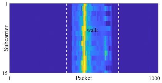
Figure 6. Quasi-envelope image containing single motion interval.

4.3. Segmentation Using Improved Otsu Algorithm

Figure 7a shows the histogram of the quasi-envelope, which exhibits a bimodal distribution. It can be seen that the grayscale values in the dynamic region no longer overlap with those in the static region, which paves the way for effective motion segmentation. Unfortunately, the classical Otsu method still fails to yield an appropriate threshold. As indicated by the yellow dashed line in Figure 7a, the computed threshold is erroneously located within the motion region. Figure 7b further shows the segmentation result using classical Otsu method; it can be seen that a large part of the motion region being misclassified as the static background.

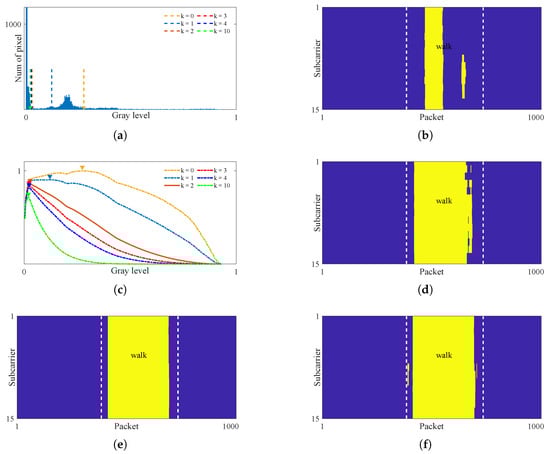
Figure 7. Segmentation of quasi-envelope. (a) Histogram and threshold. (b) Segmentation results using classical Otsu method $(k=0)$. (c) Impact of parameter k on threshold calculation. (d) Segmentation results with $k=1$. (e) Segmentation results with $k=2$. (f) Segmentation results with $k=10$.

Upon re-examining the gray level histogram of the quasi-envelope image, it can be seen that the gray level values of the static region are highly concentrated near zero, while the distribution of the dynamic region exhibits a pronounced heavy-tailed characteristic. This leads to a substantial imbalance in variance between the two regions. For example, in Figure 6, the variance of the static region is $1.37\times {10}^{-4}$, while that of the motion region is $1.90\times {10}^{-2}$. Since the classic Otsu method performs poorly when the variances of the foreground and background differ greatly, the computed segmentation threshold will inevitably deviate from the optimal value.

To address the aforementioned issue, we introduce an improved Otsu algorithm. The basic rationale stems from two observations: first, the degree of CSI fluctuations caused by environmental noise differs significantly from those induced by human motion. second, the quasi-envelope enhances dynamic region homogeneity. As a result, the gray level values of dynamic regions are distributed over a range far from zero, while those of static regions converge near zero. It follows that an appropriate threshold for distinguishing between stationary and motion regions should lie very close to zero.

Recall that the core of the classical Otsu method lies in calculating the inter-class variance, which can be expressed as:

$$V_g=p_s\left(g\right){\mu }_s^2\left(g\right)+p_d\left(g\right){\mu }_d^2\left(g\right)$$

(8)

where $p_s\left(g\right)$ and $p_d\left(g\right)$ are the probabilities of the foreground and background, respectively, ${\mu }_s\left(g\right)$ and ${\mu }_d\left(g\right)$ are the mean values of the foreground and background, respectively. Figure 7c present the calculated inter-class variance curve in yellow dot line. It can be observed that, due to the significant difference between the foreground and background, the gray level corresponding to the maximum inter-class variance is not an ideal segmentation threshold (the optimal threshold is approximately $0.025$).

Therefore, we further emphasize the gray level of the optimal threshold by introducing a weighted item ${\left(1-g\right)}^k$, where g denotes a specified gray level, and k is a non-negative integer. Then, the segmentation threshold can be written as follows:

$$g^{*}=arg\underset{0<g<L-1}{max}\left\{{\left(1-g\right)}^k{V}_g\right\}$$

(9)

where L is the total number of gray levels in the image to be segmented. Compared with classical Otsu method, the weight term ${\left(1-g\right)}^k$ ensures that the computed threshold close to the maximum grayscale value of the static region while maximizing the inter-class variance. Given that $\left(1-g\right)\le 1$, a larger k shifts the threshold toward zero, and a smaller k causes it to approach the classical Otsu threshold. Specifically, the algorithm simplifies to the classical Otsu method when $k=0$. Consequently, a large k promotes over-segmentation, whereas a small k leads to under-segmentation.

Figure 7c illustrates the effect of the weighting term on threshold calculation, where the peaks for different k values are marked by triangles in different colors. It can be seen that the weighting term emphasizes the value of the gray level itself. As the value of k increases, the peak position gradually shifts toward the lower gray levels. Figure 7a shows the corresponding thresholds with colored dashed lines. When $k=1$, the weighting term is insufficient to fully correct the threshold deviation caused by the large variance difference between foreground and background. As a result, although the integrity of the segmented motions is significantly better than that achieved by the classical Otsu method, considerable under-segmentation remains, as shown in Figure 7d. For $k\ge 2$, the segmentation threshold moves closer to the boundary between motion and static regions, further improving the integrity of motion regions, as shown in Figure 7e,f. However, merely increasing k cannot fully address under-segmentation. For instance, at $k=10$, the start and end parts of the motion region still cannot be effectively segmented, while unnecessary computational overhead is introduced. Moreover, an excessively large k significantly increases the risk of over-segmentation, which is more problematic than under-segmentation.

Therefore, the value of k should be chosen to balance between computational efficiency with motion region integrity while avoiding severe over-segmentation. In this work, k is set to 2. The remaining under-segmentation is addressed by the iterative segmentation algorithm detailed in Section 4.5.

4.4. Stopping Criterion of Iteration

By employing a quasi-envelope with enhanced homogeneity and an improved Otsu segmentation algorithm, largely complete motion regions were achieved. However, due to the relatively low speed and intensity of human movement during the start and end phases of human motion, some mis-segmentation remains in the results. The histogram further demonstrates that the gray values at the start and end of the motion closely resemble to those in static regions, leading to their misclassification as background. When a CSI stream contains multiple movements with significant amplitude differences, the aforementioned problem also arises. As discussed in Section 3.3, iterative segmentation shows significant promise for mitigating the under-segmentation issue and improving the completeness of motion intervals. A key challenge, however, is accurately determining the stopping criterion for the iteration.

It is evident that if the segmented static region contains no motion area, no further segmentation is required. Conversely, if motion regions remain present, additional segmentation remains necessary. For clarity, we classify these two types of CSI data as static-only and dynamic-included, respectively. Subsequently, we elaborate on the use of a Seeded Region Growing (SRG) algorithm to addresses the binary classification problem, thereby establishing a robust stopping criterion for the iterative segmentation process.

The SRG algorithm initiates from a set of seed pixels and iteratively incorporates neighboring pixels that meet predefined growth criteria into the expanding region until no eligible pixels remain. The algorithm relies on two key parameters: the seed points, which define the structural properties of the segmented region, and the growth threshold, which regulates the homogeneity and morphological consistency of the resulting region.

4.4.1. Seed Selection Method

Typically, the seed points are set to those pixels with special properties, such as maximum or minimum values. For the normalized variance images, the gray value distribution in the static-only variance image is random, as shown in Figure 8a. In contrast, the motion-included variance image shows a clearly clustered structure, resulting from more pronounced CSI fluctuations caused by human movement compared to those induced by ambient noise, as shown in Figure 8b. In other words, the pixels with larger grayscale values are randomly distributed in static-only variance images but cluster within the motion region in dynamic-included ones.

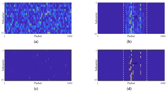
Figure 8. Seed selection. (a) Static-only variance image. (b) Dynamic-included variance image. (c) Seeds selected in static-only image. (d) Seeds selected in dynamic-included image.

Therefore, we define the seed points as those pixels with gray values satisfying the following:

$$g_i\ge \alpha \ast g_{max}$$

(10)

where $g_{max}$ denotes the maximum gray value in the variance image and $\alpha$ is a scaling coefficient not exceeding 1. For static-only images, a larger $\alpha$ value ensures stable classification by increasing the growth difficulty through seed point reduction. As for dynamic-included images, a larger growth threshold is adopted to lower the resulting difficulty, thereby promoting the growth of large motion-related regions.

Figure 8c,d show the selected seeds as yellow markers for $\alpha =1$. It can be seen that the selected seed points in the static-only image are randomly distributed across each row, whereas in the dynamic-included image, they are concentrated in specific columns within the motion region. In practice, we further randomize the order of the subcarriers. This operation significantly enhances the randomness of seed point distribution in static-only images. Conversely, the impact on dynamic-included images is limited, as their seed points are primarily distributed in columns. When region growing starts from these seed points, it is obvious that the former result is meaningless, while the latter one should be motion-related.

4.4.2. Adaptive Growth Threshold Calculation

During the growth process, the grayscale difference is adopt as the similarity criterion. Specifically, pixels in the variance image satisfying $\left|g_i-g_s\right|\le t{h}_{grow}$ are incorporated into the growing region. Notice that the purpose here is purely to distinguish between static-only and dynamic-included data; thus, we abide by the following principles: $t{h}_{grow}$ for static-only image should be as small as possible, which makes it difficult to grow a large-area motion-independent region. On the contrary, $t{h}_{grow}$ for dynamic-included image should be appropriately larger, facilitating the growth of large motion-related regions.

To this end, we resort to the gray distribution of the variance image. As shown in Figure 9, after histogram equalization, the Cumulative Distribution Function (CDF) curve of the static-only image is nearly linear, while the CDF curve of dynamic-included image is a broken line when the grayscale is small. If we pick the smallest $\beta$ nan-zero values $\left[c_1,c_2,\cdots c_{\beta },\right]$ in the CDF curve and calculate the mean value of corresponding gray values $\left[g_1,g_2,\cdots g_{\beta },\right]$, the value of the static-only image is significantly smaller than that of dynamic-included image. Thus, a satisfactory growth threshold can be obtained according to a reasonable $\beta$, which can be written as follows:

$$t{h}_{grow}=avg\left(g_1,g_2\cdots g_{\beta }\right)$$

(11)

The first non-zero gray level in the CDF is much higher for dynamic-included images than for static-only images. Consequently, a relatively small $\beta$ value is sufficient to meet the aforementioned criterion, making it far more difficult to form large homogeneous regions in static-only images than in dynamic-included ones. In Figure 9, the growth thresholds are indicated by the blue and orange arrows when $\beta =5$. The values of static-only and dynamic-included images are $0.04$ and $0.47$, respectively, with the former being significantly smaller. Compared with a fixed value, the growth threshold is calculated based on the characteristics of the variance image itself, which can adapt well to the distinct variance magnitudes caused by different human motions.

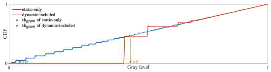
Figure 9. Calculation of growth threshold.

4.4.3. Classification Result Output

Figure 10a,b present the growth results. It can be seen that the regions grown in the static-only image are small-area and randomly distributed. In contrast, those in the dynamic-included image are larger-area and located in the motion region. To obtain the final result, we apply morphological processing to the resulting regions and compute the column-wise mean. As Figure 10c,d show, if all values in the sequence are below a predefined classification threshold $t{h}_{det}$, the CSI is classified as static-only. Otherwise, it is categorized as dynamic-included.

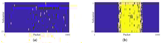
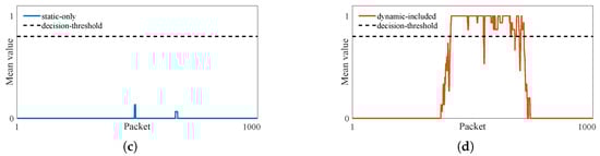
Figure 10. Illustration of the final classification result. (a) Growth result of static-only CSI. (b) Growth result of of dynamic-included CSI. (c) Column-wise mean series of static-only CSI. (d) Column-wise mean series of dynamic-included CSI.

It is worth noting that although motion detection is affected by parameters $\alpha$, $\beta$, and $t{h}_{det}$, the accuracy remains robust over a wide range of their values. A detailed analysis of this robustness is provided in Section 5.3.2.

4.5. Example of Iterative Segmentation Algorithm

Building upon the previous discussion, the complete iterative segmentation algorithm can be described as follows:

Step 1.

Calculate the quasi-envelope image $I_{qe}$ according to the amplitude image $I_{amp}$;

Step 2.

Use improved Otsu method to segment $I_{qe}$ and obtain the static regions $\left[S^1,S^2,\cdots ,S^m\right]$ and dynamic regions $\left[D^1,D^2,\cdots ,D^n\right]$;

Step 3.

Utilize motion detection method to divide $\left[S^1,S^2,\cdots ,S^m\right]$ into static-only part $\left[S_{so}^1,S_{so}^2,\cdots ,S_{so}^p\right]$ and dynamic-included part $\left[S_{di}^1,S_{di}^2,\cdots ,S_{di}^q\right]$, where $m=p+q$;

Step 4.

If $\left[S_{di}^1,S_{di}^2,\cdots ,S_{di}^q\right]=⌀$, jump to Step 5. Otherwise, recompute the quasi-envelope image $I_{qe}^j$ corresponding to each $S_{di}^j$ using $I_{amp}$, then merge $I_{qe}^j\left(1\le j\le q\right)$ to a new composite image and repeat Steps 2 through 4.

Step 5.

Merge the motion regions belonging to the same activity according to the static interval threshold ${th}_s$, remove the pseudo motion region with too short duration based on the motion duration threshold ${th}_m$, and finally, obtain all motion regions.

Figure 11 details the workflow of the proposed algorithm, using the two-motion-region scenario from Figure 4a as an example.

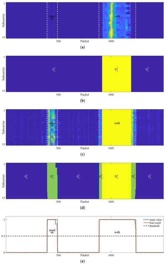
Figure 11. Illustration of multi-motion segmentation. (a) Quasi-envelope image containing two motion regions. (b) First round segmentation result. (c) Re-calculated quasi-envelope images of regions $S_1^1$ and $S_1^2$. (d) Second round segmentation result. (e) Output of segmentation result.

Firstly, the quasi-envelope image is calculated in order to enhance the homogeneity of dynamic regions, as shown in Figure 11a. Then, the improved Otsu algorithm is used to segment the quasi-envelope image. As Figure 11b shows, two static regions $\left[S_1^1,S_1^2\right]$ and a dynamic region $\left[D_1^1\right]$ are obtained. Here, the subscripts 1 is used to distinguish the round of segmentation, while the superscripts 1 and 2 indicate the numbering of static or dynamic regions in each segmentation result. It can be seen that most pixels of the walking region have been segmented.

Next, the motion detection method is employed to re-analyze regions $S_1^1$ and $S_1^2$, respectively, and both regions are judged as motion-included. Thus, we re-calculate the quasi-envelope corresponding to $S_1^1$ and $S_1^2$, as shown in Figure 11c.

Then, we merge the two new quasi-envelope images and re-segment them using the improved Otsu algorithm; the result is shown in Figure 11d. Three new static regions are obtained, including $S_2^1$, $S_2^2$, and $S_2^3$. Additionally, the results reveal three new motion regions: an independent standing-up region $D_2^1$, along with regions $D_2^2$ and $D_2^3$ corresponding to the start and end parts of walking region.

Subsequently, we assess whether the three newly identified static regions contain any motion. As all three regions are confirmed to be static-only, the iterative segmentation process terminates at this point. Then, the three motion segments, $D_2^1$, $D_2^2$, and $D_2^3$ belonging to the walking motion event are merged based on the motion interval threshold. Finally, the column-wise mean series is computed and compared with a predefined threshold, where values exceeding the threshold are treated as the human motion interval, as illustrated in Figure 11e.

5. Performance Evaluation

5.1. Experiment Setup

To verify the effectiveness of the proposed method, we conducted experiments in two real scenarios, including a dormitory and a laboratory, and the floor plans are shown in Figure 12. In the experiment, a TP-Link WDR5600 router was used as the transmitter, and a Lenovo X200 laptop equipped with an Intel 5300 NIC card was used as the receiver. Meanwhile, a well-known modified firmware, CSI Tool, was used to collect CSI data. The system worked in 2.4 GHz frequency band, and the data transmission rate was set to 100 packets/s.

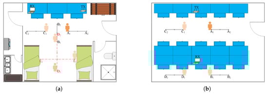
Figure 12. The floor plan of experiment scenarios. (a) Dormitory. (b) Laboratory.

Three types of CSI data were collected: static-only data, single-motion-included data, and multi-motions-included data. Specifically, we collected static-only data with a duration of 10 s in two scenarios. For single-motion-included data, we asked five volunteers to complete six actions, including walking, stepping, squatting, waving, kicking, and sitting down in scenario (a). Among them, the walking trajectories are shown as the solid black lines in Figure 12a, while the other five in situ actions were completed in positions $A_1$, $B_1$ and $C_1$. Meanwhile, the volunteers also completed the walking action in scenario (b), and the specific trajectory is shown by the solid black lines in Figure 12b. In addition, we collected multi-motions-included data that contained five independent activities. The volunteers completed the following activity sequence in scenario (a): standing up→walking→drinking→walking→sitting down. The motion trajectory is shown by the red dotted line in Figure 12a. Between adjacent actions, the volunteers remained still for a while. In order to ensure the data quality, the specific rules had been explained to the volunteers in detail, and voice prompts were played during data collection.

The testing was conducted on a desktop equipped with an Intel Core i7-12700F CPU, 32 GB of RAM, and an NVIDIA GeForce RTX 3070 GPU. In terms of the software environment, all experiments were performed in MATLAB 2024b, except for the baseline method DeepSeg, which was implemented in Python 3.13.

5.2. Evaluation Metrics

As described in Section 3.3, accurately distinguishing between static-only and motion-included data is crucial for the quality of the final motion segmentation results. For clarity, we refer to this distinction process as motion detection and the subsequent extraction of motion intervals as motion segmentation.

Obviously, motion detection can be formulated as a binary classification problem. Consequently, we adopt the traditional False Positive Rate (FPR) and False Negative Rate (FNR) to evaluate the motion detection accuracy, which is defined as follows:

$$\begin{array}{cc}\hfill FPR& ={\displaystyle \frac{NumofFP}{NumofTN+NumofFP}}\hfill \\ \hfill FNR& ={\displaystyle \frac{NumofFN}{NumofTP+NumofFN}}\hfill \end{array}$$

(12)

Here, True Positive (TP) and True Negative (TN) denote the correct classification of motion-included and static-only CSI data, respectively; False Positive (FP) refers to static-only CSI data misclassified as motion-included; and False Negative (FN) indicates the inverse misclassification scenario.

For motion segmentation, we firstly employ Temporal Intersection Over Union (T-IoU) to evaluate the validity of segmented motion intervals, and we treat the segmented motion intervals with a T-IOU value exceeding 50% as True Motion Intervals (TMI), while those below this threshold are classified as False Motion Intervals (FMI). Building on this criterion, Event-level False Positive Rate (E-FPR) and Event-level False Negative Rate (E-PNR) are further introduced to assess the proportions of false motion intervals and missed motion intervals, respectively. These metrics are defined as follows:

$$\begin{array}{cc}\hfill E\text{-}FPR& ={\displaystyle \frac{NumofFMI}{NumofTMI+NumofFMI}}\hfill \\ \hfill E\text{-}FNR& ={\displaystyle \frac{NumofMMI}{NumofTMI+NumofMMI}}\hfill \end{array}$$

(13)

where Missed Motion Interval (MMI) denotes unsegmented ground-truth motion intervals. It can be seen that E-FPR quantifies spurious segmented motion events, while E-FNR measures the missed true motion events. This methodology effectively mitigates the impacts of static and dynamic frame imbalance, thereby better meeting the practical requirements of real-world scenarios.

For temporal accuracy evaluation, the Motion Start-point Segmentation Error (MSSE) and Motion End-point Segmentation Error (MESE) are employed to quantify temporal deviations, which can be described as follows:

$$\begin{array}{cc}\hfill MSSE& =\left|T{S}_{seg}-T{S}_{gt}\right|\hfill \\ \hfill MESE& =\left|T{E}_{seg}-T{E}_{gt}\right|\hfill \end{array}$$

(14)

Here, $T{S}_{seg}$ and $T{E}_{seg}$ denote the segmented start point and end point, respectively, and $T{S}_{gt}$ and $T{E}_{gt}$ denote the ground-truth motion start and end point, respectively.

5.3. Validation of Human Motion Detection Algorithm

In this subsection, we use all the collected data to evaluate the effectiveness of the proposed method in distinguishing between static-only and dynamic-included CSI data.

5.3.1. Impact of CSI Feature

Owing to the inherent denoising capability of the CSI ratio, its amplitude, phase, and complex-plane distance can all be utilized for motion perception. For comparison, we also calculated their corresponding quasi-envelope features to evaluate the motion detection performance. The results are shown in Figure 13.

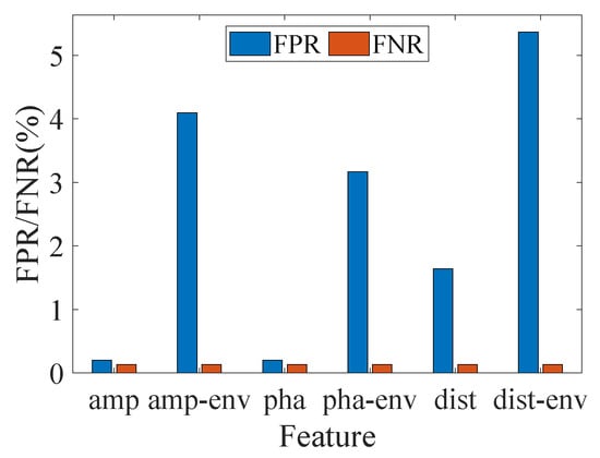
Figure 13. Detection results using different features.

As Figure 13 shows, the system achieves satisfactory accuracy with the direct use of variance images for motion detection. Specifically, using variance in either amplitude or phase yields optimal performance, with an FPR of $0.20\%$ and an FNR of $0.13\%$. These results validate the effectiveness and robustness of the proposed approach. However, the performance declines sharply when the quasi-envelope is adopted. As the quasi-envelope attenuates local fluctuations in the original signal, false homogeneous regions emerge in the quasi-envelope image. As a result, the FPR of the system significant increases. In contrast, for motion detection, the variance image already exhibits sufficient homogeneity in motion regions. Consequently, the quasi-envelope yields no significant reduction in FNR while introducing unnecessary computational overhead. This further validates the importance of feature selection in WiFi sensing. In the following discussing, we select the variance of CSI ratio amplitude for human motion detection.

5.3.2. Impact of SRG Parameters

For the motion detection algorithm, the key parameters are automatically determined based on the statistical features of variance images. Specifically, the seeds are selected as the pixels with gray values exceeding $\alpha$ times the maximum. The growth threshold is defined as the mean of the smallest $\beta$ values in the CDF. Finally, the CSI is classified by comparing the column-wise mean series with the detection threshold $t{h}_{det}$. Fixing the number of subcarriers at 15, a systematic evaluation was conducted to assess the impacts of above three parameters, with $\alpha$, $\beta$, and $t{h}_{det}$ ranges configured as $0.95$–$1.00$, 1–10, and $0.50$–$1.00$, respectively. The FPR and FNR results are presented in Figure 14 and Figure 15. Here, the warm tones (e.g., red) indicate large values, and the cool tones (e.g., dark blue) indicate low values.

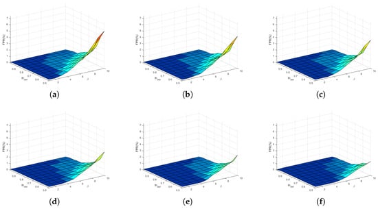
Figure 14. FPR using different parameters. (a) $\alpha =0.95$, (b) $\alpha =0.96$, (c) $\alpha =0.97$, (d) $\alpha =0.98$, (e) $\alpha =0.99$, (f) $\alpha =1.00$.

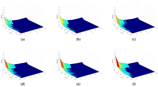
Figure 15. FNR using different parameters. (a) $\alpha =0.95$, (b) $\alpha =0.96$, (c) $\alpha =0.97$, (d) $\alpha =0.98$, (e) $\alpha =0.99$, (f) $\alpha =1.00$.

When $\alpha$ is fixed, the FPR is proportional to $\beta$ but inversely proportional to $t{h}_{det}$, whereas the FNR is negatively correlated with $\beta$ but positively with $t{h}_{det}$. This relationship is most evident in Figure 14a and Figure 15f. A larger $\beta$ value indicates a more lenient region growing criterion, allowing more adjacent pixels to be merged. For static-only data, this operation results in more false motion regions, thereby increasing the FPR. For dynamic-included data, however, this operation promotes the formation of homogeneous regions, thereby reducing the FNR. Furthermore, an increase in the $t{h}_{det}$ value represents a stricter motion detection criterion, which increases the FNR while decreasing the FPR.

Furthermore, the overall trend in Figure 14 demonstrates that increasing the $\alpha$ value not only effectively reduces the FPR under fixed $\beta$ and $t{h}_{det}$ conditions but also enables the system to maintain a low FPR level across a wider range of $\beta$ and $t{h}_{det}$ parameters. A larger $\alpha$ value means fewer seed points in the CSI variance image, which increases the difficulty of region growing. Therefore, larger growth threshold and motion detection criteria can be adopted without altering the classification performance. Compared with the FPR, Figure 15 shows an inverse relationship between the FNR and $\alpha$. A noteworthy finding is that when $\alpha =1$, both the FPR and FNR can be maintained at low levels, even as $\beta$ and $t{h}_{det}$ vary over wide ranges (e.g., $\beta \in [3,7]$ and $t{h}_{det}\in [0.6,0.9]$). This demonstrates that the motion detection algorithm is parameter-robust. In this work, $\alpha$, $\beta$ and $t{h}_{det}$ are set to 1, 5, and 0.8, respectively.

Furthermore, we investigated the impact of the number of subcarriers on the optimal SRG parameters. With parameters fixed ($\alpha =1$, $\beta =5$, $t{h}_{det}=0.8$), motion detection accuracy was reevaluated using 30 to 90 subcarriers. As Figure 16 shows, the accuracy remains stable within a moderate range (e.g., 30, 45 subcarriers), confirming the method’s parametric robustness. However, performance degrades significantly with excessive subcarriers (e.g., 75, 90 subcarriers), as the inclusion of poor subcarriers with low static stability and motion sensitivity severely interferes with detection. Using the same parameter-sweeping method described earlier, we identified the optimal performance for 60, 75, and 90 subcarriers. The FPR and FNR are (0.26%, 0.18%), (1.20%, 0.56%), and (2.12%, 1.16%), respectively, all of which are inferior to the performance achieved with 15 subcarriers. This further underscores the critical importance of subcarrier selection.

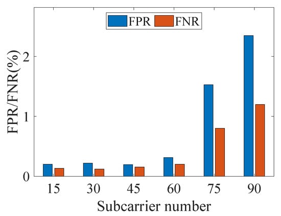
Figure 16. Detection results using different subcarriers.

5.3.3. Impact of CSI Length and Static–Dynamic Ratio

To verify the robustness of the method, the collected CSI data were artificially truncated with controlled proportions. For static-only classes, this operation changed the length of CSI data, whereas for motion-included classes, it modified static-dynamic ratios. The truncated data were then re-evaluated for motion detection, with results shown in Figure 17.

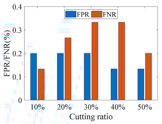
Figure 17. Detection results under varying data length and static–dynamic ratio.

Notably, the system maintains consistently low FPR and FNR. The core discriminative mechanism depends on whether sufficiently large homogeneous regions can be grown in the CSI-ratio image, as described in Section 4.4. In static-only CSI data, noise-induced stochastic fluctuations are independent of data length, which inherently prevent the formation of such large regions. Conversely, the coherent fluctuations caused by human motion naturally establish homogeneous regions in the motion-included image. This fundamental difference allows the system to maintain stable detection accuracy despite variations in data length and static–dynamic ratio.

5.4. Performance of Human Motion Segmentation

Since the presence of motion has been accurately determined, CSI data containing only a single motion instance are employed to assess the system’s motion segmentation performance.

5.4.1. Overall Performance

For comparison, five representative human motion segmentation methods are selected as baselines, including both unsupervised and learning-based approaches.

(1) WISH [6]: A lightweight threshold-based human motion segmentation method that utilizes correlating property of CSI in both time and frequency domain.

(2) AR-Alarm [3]: An environment-adaptive activity segmentation method that use the normalized standard deviation of phase difference as a robust CSI feature.

(3) LightSeg [16]: A lightweight method that detects the end of human motion using a predefined threshold and then decides the appropriate threshold based on the linear traversal of the CSI stream.

(4) MoSeFi [15]: A during-robust human motion segmentation method that employs a combined variance metric based on the complementarity between the real and imaginary parts of the CSI ratio.

(5) DeepSeg [18]: A learning-based method that adopted a CNN architecture. This method divides the continuous CSI streams into equal sized bins and classifies these bins into four states, including static-state, start-state, motion-state, and end-state. Finally, the start and end motion points are determined as the middle points of start-state and end-state bins, respectively.

As WISH and AR-Alarm do not include a subcarrier selection module, we integrated the same curvature distance-based method used in MoSeFi, and the improved versions are denoted as WISH⁺ and AR-Alarm⁺, respectively. We evaluated WISH⁺, AR-Alarm⁺, and LightSeg across multiple window lengths (0.5 s, 1 s, 1.5 s) and selected their best-performing results for comparison. For our prior work on MoSeFi and the open-source method DeepSeg, we adopted the parameters reported in their original publications. The system performances are presented in Table 2. Here, the abbreviations WinSize and RT denote the window size used in testing and the average run time for a single CSI data unit, respectively.

Table 2. System performance compared with other methods.

Method	WinSize (s)	E-FPR (%)	E-FNR (%)	MSSE (s)	MESE (s)	RT (s)
WISH+	1.00	0.78	1.00	0.27	0.29	0.38
AR-Alarm+	1.00	0.89	1.34	0.48	0.57	0.12
LightSeg	1.00	1.32	0.84	0.42	0.46	0.17
MoSeFi	0.50	0.78	0.67	0.22	0.31	0.13
DeepSeg	1.00	0.21	0.25	0.32	0.38	0.06
Ours	0.50	0.33	0.20	0.26	0.29	0.26
Ours-var	0.50	1.71	0.60	0.37	0.32	0.22
Ours-Otsu	0.50	1.36	0.67	0.38	0.34	0.28

Owing to the well-constructed quasi-envelope feature and the iterative segmentation algorithm, the proposed method achieves excellent motion segmentation performance, with an E-FPR = 0.33% and E-FNR = 0.20% respectively. This performance surpasses that of methods based on variance or correlation coefficient thresholds and is comparable to deep learning-based approaches. Moreover, the accurate motion detection algorithm ensures the iterative process terminates appropriately, effectively mitigating both over-segmentation and under-segmentation. Consequently, our method guarantees accurate counting of motion events and precise identification of their boundaries.

In terms of real-time performance, our method surpasses the correlation-based WISH because it avoids computing complex correlation coefficients. However, as it needs to process variance images composed of multiple time series, its running time is higher than that of single-series-based methods (e.g., AR-Alarm⁺, MoSeFi, LightSeg). Although the learning-based DeepSeg achieves the shortest running time, it is crucial to note that this result does not include the time costs for data labeling and model training. If included, its total computational burden would be the largest.

The time distribution across different stages of our method is further shown in Figure 18, where PP, SS, EC, MD, and MS denote preprocessing, subcarrier selection, envelope calculation, motion detection, and motion segmentation, respectively. It can be seen that the preprocessing stage, which processes all CSI ratio series, accounts for the majority of the computational overhead, highlighting the importance of the subcarrier selection module. Additionally, constrained by the efficiency of the SRG algorithm, the motion detection stage also consumes a considerable proportion of time. Comparatively, the envelope calculation and the iterative Otsu segmentation processes require relatively less time. For a 15 s data sample, the average run time of our method in the MATLAB 2024b. environment is 0.26 s, which meets the requirements of most real-time applications. The real-time performance could be further enhanced by implementing the method in a more efficient programming language like C++.

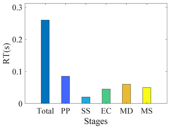
Figure 18. Running time distribution across different stages.

5.4.2. Importance of Quasi-Envelope Calculation

To clarify the role of the quasi-envelope feature, we conducted an ablation study. With all other modules and parameters fixed, we applied the improved Otsu-based iterative segmentation algorithm directly to the raw variance images. The results are presented in Table 2, where this ablated version is denoted with the suffix -var for clarity.

It can be seen that when raw variance images are used for segmentation, the system’s overall performance degrades substantially, contrasting sharply with the motion detection results in Section 5.3. Without the homogeneity enhancement provided by the quasi-envelope, motion integrity is disrupted during single segmentation round, leading to severe motion fragmentation. These results underscore the critical importance of tailoring CSI feature selection to the specific task for optimal system performance.

5.4.3. Significance of Improved Otsu Algorithm

In a similar ablation study, we evaluated system performance by applying the classical Otsu algorithm for iterative segmentation on the quasi-envelope images, which is denoted as Ours-Otsu in Table 2. The results show significant performance degradation.

This is because the substantial variance difference between foreground and background causes the classical Otsu threshold to deviate consistently from the optimum. This deviation reduces the completeness of the segmented motion regions in each round, leading to severe under-segmentation. To compensate, the system requires more iterations, as reflected in the elevated RT values. The increased iteration count, in turn, raises the probability of erroneously merging or discarding motion sub-intervals in later stages, ultimately degrading both segmentation accuracy and temporal precision.

5.4.4. Impact of Prominence Threshold

In the computation of the quasi-envelope, a prominence threshold $t{h}_{pro}$ is applied to eliminate insignificant peaks, enhancing the homogeneity of the motion regions. Here, we varied $t{h}_{pro}$ from $0.02$ to $0.20$ to evaluate the influence of the prominence threshold, and the experimental results are illustrated in Figure 19.

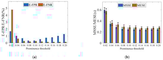
Figure 19. Segmentation results using different peaks. (a) E-FPR and E-FNR. (b) MSSE and MESE.

Evidently, excessively high or low prominence thresholds adversely affect motion segmentation performance. When $t{h}_{pro}$ is set too large, fewer peaks are selected. Consequently, the distance between adjacent peaks increases. Recall that we only perform interpolation between nearby peaks according to a distance threshold. For distant peaks, we treat them as belonging to different motion intervals and use the original variance series between these peaks to represent the envelope. Conversely, if $t{h}_{pro}$ is set too small, spurious peaks with low prominence are incorporated into the computation. Both of these conditions cause the calculated quasi-envelope to more closely approximate the original series, thereby leading to fragmentation of the segmentation results. The conventional single time-threshold approach is inadequate to fully resolve such issues, which reduces the overall accuracy of the system. In this work, $t{h}_{pro}$ was set to $0.08$.

5.4.5. Impact of Subcarrier Number

Considering frequency-selective fading, a subset of subcarriers was selected for motion segmentation. Figure 20 shows the system performance across varying numbers of subcarriers.

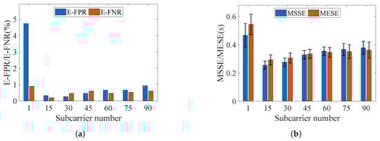
Figure 20. Segmentation results using different subcarriers. (a) E-FPR and E-FNR. (b) MSSE and MESE.

It can be seen that proper subcarrier selecting can effectively improve the system performance. For example, using 15 subcarriers instead of all subcarriers decreases the E-FPR and E-FNR from $0.93\%$ and $0.60\%$ to $0.33\%$ and $0.20\%$, respectively. By removing subcarriers that exhibit poor static stability or low dynamic sensitivity, the threshold determination is simplified, thereby improving segmentation accuracy. Furthermore, the reduction of subcarriers lower the computational overhead, which enhances real-time processing capability.

However, an excessive reduction in the number of subcarriers is detrimental to system performance. For example, when only a single subcarrier is selected, the quasi-envelope image degenerates into a one-dimensional time series. The absence of inter-subcarrier complementarity leads to inadequate information for motion capture, which in turn causes a noticeable deterioration in the performance of all evaluation metrics.

5.4.6. Impact of Motion Interval Location

To evaluate the influence of motion interval location on segmentation performance, the static interval preceding or following the motion in original CSI data was trimmed, thereby generating two new datasets: motion-static set, which retains only post-motion static interval, and static-motion set, which retains only pre-motion static interval. Figure 21 shows the system performance on the two modified datasets.

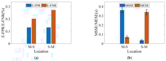
Figure 21. Segmentation results under different locations of motion. (a) E-FPR and E-FNR. (b) MSSE and MESE.

Compared with the original static–dynamic–static dataset, the system performance is robust to the location of the motion interval. As described in Section 4, the CSI ratio is treated as an entire image, and the segmentation threshold is derived from the statistical characteristics of the variance quasi-envelope image rather than from pre-collected static interval data or trained parameters. When the location of the motion interval changes, the gray-value distribution characteristics of the quasi-envelope image do not undergo significant alterations. Therefore, the improved Otsu algorithm can still identify an appropriate segmentation threshold. Meanwhile, the process of data trimming removes spurious motion intervals in static regions, thereby lowering the E-FPR, MSSE and MESE of the system.

5.4.7. Impact of Motion Interval Number

To evaluate the system performance in multi-motion scenarios, we selectively truncated the original CSI series that included five motion intervals. Ultimately, five new datasets were constructed, with each CSI series containing from 1 to 5 motion intervals. The experimental results obtained from the new dataset are presented in Figure 22.

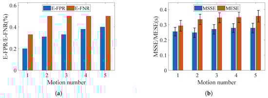
Figure 22. Segmentation results across varying motion counts. (a) E-FPR and E-FNR. (b) MSSE and MESE.

Clearly, an increase in $N_{\mathrm{motion}}$ raises the difficulty of motion segmentation. Nevertheless, the system maintains strong robustness due to the well-designed motion detection algorithm and the iterative motion segmentation strategy. Even with $N_{\mathrm{motion}}=5$, the E-FPR and E-FNR remain as low as $0.40\%$ and $0.50\%$, respectively, while the MSSE and MESE exhibit only a slight increase to $0.28$ s and $0.36$ s. These results indicate that the system can effectively handle the challenges posed by multiple motions.

To further demonstrate the advantages of iterative segmentation, we also evaluated the system performance under a single-pass segmentation process. The results indicate that a single segmentation pass is insufficient to ensure the complete acquisition of all motion intervals. For example, when $N_{\mathrm{motion}}=2$, the E-FNR increases significantly to $40\%$, and when $N_{\mathrm{motion}}=5$, it further rises to $55\%$. In contrast, the iterative segmentation algorithm performs motion detection on each segmented sub-region. If motion is detected, the sub-regions are further re-segmented. This iterative algorithm effectively mitigates errors caused by variations in motion strength, ensuring accurate segmentation of all motion intervals.

5.5. Discussion

Performance in unseen environment: To validate the applicability of the proposed method in a new environment, we conducted an additional experiment using an public CSI dataset [25]. This dataset was collected in a furnished room with a Sagemcom-2704 router and a desktop equipped with an Intel 5300 card. The sampling rate was set as 100 Hz. It includes 12 types of human-to-human activities performed by 40 participant pairs, ranging from large-scale motions (e.g., pushing) to small-scale ones (e.g., handshaking). The segmentation process employed the same parameter set as used in the self-collected dataset experiments, and the system performance is shown in Table 3. It can be seen that the results closely align with the performance on our self-collected dataset, demonstrating that the proposed algorithm exhibits strong environmental adaptability.

Table 3. System performance on unseen environment and noise-contaminated datasets.

Dataset	E-FPR (%)	E-FNR (%)	MSSE (s)	MESE (s)
Open human-to-human dataset	0.38	0.25	0.28	0.31
Fan-noise-contaminated dataset	3.06	4.00	0.63	0.71
Robot-noise-contaminated dataset	22.10	18.00	0.92	1.12

Distinguish between the motion of multi-persons. We also evaluated the method’s ability to discriminate the source of CSI fluctuations using the human-to-human dataset. However, limited by the narrow bandwidth of commercial WiFi and the inherent lack of discriminative power in variance, our method accurately captures human motion but cannot identify the specific individual causing the variations. Several studies have demonstrated multi-person discrimination under specific conditions, suggesting a viable path forward. Therefore, our future work will focus on developing more accurate signal propagation models or integrating deep learning to better discriminate motions from different individuals, thereby providing a stronger foundation for advanced applications.

Challenge of noisy environment. We employed a rotating fan with blade radius of 15 cm and a randomly moving robot with height 70 cm as noise sources, collecting 100 instances of CSI data containing human walking motion. As shown in Table 3, system performance is directly affected by the noise level, with all evaluation metrics deteriorating. First, noise distorts the CDF of the variance image. As the growth threshold in SRG is derived from the first $\beta$ non-zero values of the CDF, this alteration would narrow the difference between the thresholds for static-only and dynamic-included images, ultimately leading to detection failure. Second, noise increases the variance of the static background. This prevents the formation of an envelope image with a bimodal histogram via the prominence threshold, thus causing segmentation failure. To address this issue, future work will explore integrating advanced signal processing techniques, such as utilizing both 2.4 GHz and 5 GHz frequency bands, convergence-based termination criteria, and dimensionality reduction [26,27,28], to enhance system robustness under noisy conditions.

6. Conclusions

With the wide deployment of mobile network, environment perception using wireless signal has received increasing attention. In this paper, we proposed a training-free and environment-robust human motion segmentation system based on commercial WiFi devices. By treating the collected CSI as a whole image rather than individual time series, we employ the quasi-envelope to characterize the difference in CSI fluctuations between human motion and stationary states and design an iterative segmentation algorithm to accommodate varying motion intensities. To improve the efficiency and accuracy of individual segmentation rounds, an improved Otsu algorithm is adopted to obtain a threshold that better meets practical segmentation needs. Furthermore, a well-designed motion detection algorithm establishes a precise criterion for iterative termination, which effectively prevents over-segmentation. Extensive experimental results in real-world scenarios demonstrate the efficiency and robustness of the proposed method. Its performance meets the requirements of practical applications, thereby facilitating the practical deployment of WiFi sensing.

References

- Halperin, D.; Hu, W.; Sheth, A.; Wetherall, D. Predictable 802.11 packet delivery from wireless channel measurements. ACM SIGCOMM Comput. Commun. Rev. 2010, 40, 159–170. [Google Scholar] [CrossRef]
- Liu, W.; Gao, X.; Wang, L.; Wang, D. BFP: Behavior-free passive motion detection using PHY information. Wirel. Pers. Commun. 2015, 83, 1035–1055. [Google Scholar] [CrossRef]
- Li, S.; Li, X.; Niu, K.; Wang, H.; Zhang, Y.; Zhang, D. Ar-alarm: An adaptive and robust intrusion detection system leveraging csi from commodity WiFi. In Proceedings of the Enhanced Quality of Life and Smart Living: 15th International Conference, ICOST 2017, Paris, France, 29–31 August 2017; pp. 211–223. [Google Scholar]
- Lin, Y.; Gao, Y.; Li, B.; Dong, W. Revisiting indoor intrusion detection with WiFi signals: Do not panic over a pet! IEEE Internet Things J. 2020, 7, 10437–10449. [Google Scholar] [CrossRef]
- Qian, K.; Wu, C.; Yang, Z.; Liu, Y.; He, F.; Xing, T. Enabling contactless detection of moving humans with dynamic speeds using CSI. ACM Trans. Embed. Comput. Syst. (TECS) 2018, 17, 52. [Google Scholar] [CrossRef]
- Hang, T.; Zheng, Y.; Qian, K.; Wu, C.; Yang, Z.; Zhou, X.; Liu, Y.; Chen, G. WiSH: WiFi-based real-time human detection. Tsinghua Sci. Technol. 2019, 24, 615–629. [Google Scholar] [CrossRef]
- Zhuang, W.; Shen, Y.; Li, L.; Gao, C.; Dai, D. Develop an adaptive real-time indoor intrusion detection system based on empirical analysis of OFDM subcarriers. Sensors 2021, 21, 2287. [Google Scholar] [CrossRef]
- Gui, L.; Yuan, W.; Xiao, F. CSI-based passive intrusion detection bound estimation in indoor NLoS scenario. Fundam. Res. 2022, 3, 988–996. [Google Scholar] [CrossRef]
- Lv, J.; Man, D.; Yang, W.; Gong, L.; Du, X.; Yu, M. Robust device-free intrusion detection using physical layer information of WiFi signals. Appl. Sci. 2019, 9, 175. [Google Scholar] [CrossRef]
- Natarajan, A.; Krishnasamy, V.; Singh, M. Device-free human motion detection using single link WiFi channel measurements for building energy management. IEEE Embed. Syst. Lett. 2022, 15, 153–156. [Google Scholar] [CrossRef]
- Mesa-Cantillo, C.M.; Sánchez-Rodríguez, D.; Alonso-González, I.; Quintana-Suárez, M.A.; Ley-Bosch, C.; Alonso-Hernández, J.B. A non intrusive human presence detection methodology based on channel state information of Wi-Fi networks. Sensors 2023, 23, 500. [Google Scholar] [CrossRef]
- Jayaweera, S.S.; Ozturk, M.Z.; Wang, B.; Liu, K.R. Robust Deep Learning Based Residential Occupancy Detection with WiFi. In Proceedings of the 23rd ACM Conference on Embedded Networked Sensor Systems, Irvine, CA, USA, 6–9 May 2025; pp. 662–663. [Google Scholar]
- Yu, A.; Yuan, C.; Gao, C.; Tong, X.; Liu, X.; Xie, X.; Chen, J.; Li, K. LowDetrack: A Human Detection and Tracking System for Wi-Fi Low Packet Rates. IEEE Internet Things J. 2025, 12, 38322–38337. [Google Scholar] [CrossRef]
- Gu, Y.; Zhan, J.; Ji, Y.; Li, J.; Ren, F.; Gao, S. MoSense: An RF-based motion detection system via off-the-shelf WiFi devices. IEEE Internet Things J. 2017, 4, 2326–2341. [Google Scholar] [CrossRef]
- Wang, X.; Zhang, L.; Cheng, Q.; Shu, F. MoSeFi: Duration estimation robust human motion sensing via commodity WiFi device. Wirel. Commun. Mob. Comput. 2022, 2022, 1690602. [Google Scholar] [CrossRef]
- Chen, L.; Zheng, X.; Xu, L.; Liu, L.; Ma, H. Lightseg: An online and low-latency activity segmentation method for Wi-Fi sensing. In Proceedings of the International Conference on Mobile and Ubiquitous Systems: Computing, Networking, and Services; Springer: Berlin/Heidelberg, Germany, 2022; pp. 227–247. [Google Scholar]
- Zhang, L.; Ma, Y.; Zuo, M.; Ling, Z.; Dong, C.; Xu, G.; Shu, L.; Fan, X.; Zhang, Q. Toward Cross-Environment Continuous Gesture User Authentication with Commercial Wi-Fi. IEEE Trans. Netw. 2025, 33, 1900–1915. [Google Scholar] [CrossRef]
- Xiao, C.; Lei, Y.; Ma, Y.; Zhou, F.; Qin, Z. DeepSeg: Deep-learning-based activity segmentation framework for activity recognition using WiFi. IEEE Internet Things J. 2020, 8, 5669–5681. [Google Scholar] [CrossRef]
- Chen, S.Y.; Lin, C.L. Subtle Motion Detection Using Wi-Fi for Hand Rest Tremor in Parkinson’s Disease. In Proceedings of the 2022 44th Annual International Conference of the IEEE Engineering in Medicine & Biology Society (EMBC), Glasgow, UK, 11–15 July 2022; pp. 1774–1777. [Google Scholar]
- Zheng, N.; Liu, R.; Fan, X.; Zhang, C.; Zhang, L.; Yin, Z. SEGALL: A Unified Active Learning Framework for Wireless Sensing Data Segmentation. Proc. ACM Interact. Mob. Wearable Ubiquitous Technol. 2025, 9, 156. [Google Scholar] [CrossRef]
- Wang, W.; Liu, A.X.; Shahzad, M.; Ling, K.; Lu, S. Understanding and modeling of wifi signal based human activity recognition. In Proceedings of the 21st Annual International Conference on Mobile Computing and Networking, Paris, France, 7–11 September 2015; pp. 65–76. [Google Scholar]
- Zhuo, Y.; Zhu, H.; Xue, H.; Chang, S. Perceiving accurate CSI phases with commodity WiFi devices. In Proceedings of the IEEE INFOCOM 2017-IEEE Conference on Computer Communications, Atlanta, GA, USA, 1–4 May 2017; pp. 1–9. [Google Scholar]
- Ma, Y.; Zhou, G.; Wang, S. WiFi sensing with channel state information: A survey. ACM Comput. Surv. (CSUR) 2019, 52, 46. [Google Scholar] [CrossRef]
- Zhai, G.; Liang, Y.; Tan, Z.; Wang, S. Development of an iterative Otsu method for vision-based structural displacement measurement under low-light conditions. Measurement 2024, 226, 114182. [Google Scholar] [CrossRef]
- Alazrai, R.; Awad, A.; Baha’A, A.; Hababeh, M.; Daoud, M.I. A dataset for Wi-Fi-based human-to-human interaction recognition. Data Brief 2020, 31, 105668. [Google Scholar] [CrossRef]
- Colange, B.; Peltonen, J.; Aupetit, M.; Dutykh, D.; Lespinats, S. Steering distortions to preserve classes and neighbors in supervised dimensionality reduction. Adv. Neural Inf. Process. Syst. 2020, 33, 13214–13225. [Google Scholar]
- Lespinats, S.; Colange, B.; Dutykh, D. Nonlinear Dimensionality Reduction Techniques; Springer: Berlin/Heidelberg, Germany, 2022. [Google Scholar]
- Colange, B.; Vuillon, L.; Lespinats, S.; Dutykh, D. MING: An interpretative support method for visual exploration of multidimensional data. Inf. Vis. 2022, 21, 246–269. [Google Scholar] [CrossRef]
Disclaimer/Publisher’s Note: The statements, opinions and data contained in all publications are solely those of the individual author(s) and contributor(s) and not of MDPI and/or the editor(s). MDPI and/or the editor(s) disclaim responsibility for any injury to people or property resulting from any ideas, methods, instructions or products referred to in the content. |
© 2025 by the authors. Licensee MDPI, Basel, Switzerland. This article is an open access article distributed under the terms and conditions of the Creative Commons Attribution (CC BY) license.