Automating Signal Synchronization for Enhanced Track Monitoring in Turnouts

Abstract

The focus of this research is the automation of the synchronization process for track-recording vehicle signals in turnouts. Accurate synchronization of measurement signals is essential for assessing specific track sections—especially complex areas such as turnouts—and for enabling reliable time series for condition monitoring. Currently, the synchronization process is only partially automated, resulting in high levels of manual effort. With over 4000 turnouts on Austria’s main railways, full automation is important for ensuring efficiency and consistency of the synchronization process. Based on an analysis of 109 turnouts in the OeBB railways, the process begins with rough synchronization using mileage and curvature signals to eliminate invalid measurement runs. Subsequently, longitudinal level signals are synchronized within maintenance time blocks. These blocks include measurement runs with consistent signal characteristics between two maintenance interventions. The latest valid run then serves as reference for each block. Methods such as cumulative sum, Euclidean distance and cross-correlation are then employed to achieve fine synchronization. The results demonstrate the feasibility and efficiency of automated synchronization compared to manual methods, enabling more accurate condition assessment. This allows infrastructure managers to track turnout-specific quality indicators, integrate them into asset management systems, and develop predictive maintenance strategies.

1. Introduction

Automating signal synchronization for enhanced infrastructure monitoring in turnouts addresses the challenge of improving the accuracy and efficiency of track condition assessment through automated synchronization methods developed specifically for complex turnout geometries. Due to their complex mechanical design and exposure to concentrated loads, turnouts are among the most maintenance-intensive elements of railway infrastructure [1]. In Austria alone, there are currently more than 13,500 turnouts in operation that require regular inspections to ensure safety and reliability. Traditionally, such inspections rely on manual measurements of various dimensions and visual assessments performed at fixed intervals. While this approach is well-established, it is time-consuming and resource-intensive. It also exposes maintenance personnel to significant safety risks when working directly on the track. Furthermore, manual inspections represent the unloaded track state and depend on the operator’s subjective judgment, which limits their suitability for predictive maintenance strategies.

Track-recording vehicles are indispensable for monitoring track geometry, planning maintenance, and analyzing long-term deterioration trends [2,3,4,5,6]. However, these measurement systems only support condition-based maintenance strategies when data from successive runs are spatially synchronized with high accuracy. Especially in turnout areas, analyzing localized effects requires that identical signal features correspond to the same physical location [7]. Nevertheless, achieving such synchronicity is challenging because recorded signals are influenced by factors such as wheel slip, track wear, sensor noise, and varying vehicle speeds [8,9,10,11,12]. Consequently, measurement signals often exhibit positional distortions, including constant offsets and local stretching or compression, which obscure the evolution of individual defects and reduce the reliability of degradation modeling [10,12,13]. Although GPS-based positioning is commonly used to determine a vehicle’s location, the availability of GPS signals is severely restricted in environments such as tunnels, dense forests and mountainous regions where satellite reception is limited [9,10,14,15]. Consequently, unreliable position estimation in such environments hinders not only the synchronization of measurement signals between successive runs, but also adversely affects the accuracy of train positioning and identification [16,17,18]. For analyzing open track, conventional track quality indicators such as a standard deviation with a 200 m influence length are robust enough to deliver good results even in case of small positioning errors.

Various synchronization methods have been proposed in recent years to overcome these limitations. These approaches can be broadly classified as absolute or relative position-based methods. Absolute methods use georeferenced, predefined physical reference points (e.g., GPS-surveyed trackside markers or mileposts) to align measurements [11,19]. Relative methods, by contrast, synchronize datasets based on the similarity of their signal shapes, employing statistical or distance-based measures [20,21]. Common algorithms employ the Pearson correlation coefficient, cross-correlation, dynamic time warping (DTW) [22,23], and correlation-optimized warping (COW) [24]. While these methods improve signal synchronization, they are often computationally demanding and sensitive to measurement noise, amplitude variations, and missing data [13,25]. Therefore, developing a method that achieves high synchronization accuracy, preserves signal integrity, and operates efficiently remains an open challenge in railway data analytics. Recent studies have demonstrated the potential of physics-informed deep learning to enhance the accuracy and robustness of rail vehicle trajectory estimation, paving the way for the development of intelligent rail transit systems [26].

Over the past decade, the Institute of Railway Engineering and Transport Economics at TU Graz has focused its research on the issue of signal synchronization, particularly within turnout areas. Fellinger [8] developed the first systematic approach, applying Euclidean distance minimization to achieve accurate signal synchronization. Although this method provided precise results, it required significant computational resources and manual post-processing. Synchronization of data for a single turnout could take up to one full working day. Building upon this work, Loidolt [7] optimized the process’s computational efficiency, reducing processing time to approximately 15 min per turnout. However, manual fine adjustments were still necessary to ensure correct synchronization. More recently, Offenbacher [27] developed the first automated signal synchronization algorithm, although this was designed primarily for open track sections. While this approach demonstrated the feasibility of full automation, its performance in turnout areas was limited as the signals in these areas feature different characteristics, such as a higher density of local defects than open track sections.

Building on this research, we introduce a fully automated positioning framework tailored specifically to turnout monitoring. Doing so, we integrate statistical and distance-based synchronization techniques, such as the cumulative sum, Euclidean distance, and cross-correlation, to achieve coarse and fine synchronization. This two-step procedure minimizes computational effort while maintaining high synchronization accuracy and robustness against local distortions. Eliminating manual intervention enables scalability and significantly reduces processing time and human error, thereby enhancing data consistency across multiple inspection runs.

The goal of this research is to provide a scalable, reproducible synchronization solution that improves the reliability of assessing turnout-specific track condition. Accurate synchronization of track geometry data is essential for detecting defect evolution, supporting predictive maintenance, and integrating turnout condition indicators into infrastructure management systems. The results of this study contribute to the digitization of railway maintenance by laying the groundwork for the automated, data-driven monitoring of critical infrastructure assets.

The paper is organized as follows: Section 2 presents the data basis and preparation steps. This section includes a description of the measurement data used, the selection of relevant signals for the synchronization process, and the identification of signals that will serve as indicators for subsequent condition monitoring analyses. It also defines turnout area boundaries and outlines preprocessing procedures required before synchronization can begin. Section 2.4 introduces the proposed processing framework and details the applied synchronization methods as well as the mathematical principles underlying them. It also explains the strategy used for coarse and fine synchronization, as well as for evaluating synchronization quality. Section 3 evaluates the automated synchronization framework, analyzing measurement run validity and computational efficiency. Section 4 presents the results obtained from applying the proposed framework. Finally, Section 5 discusses the findings, highlights potential applications for predictive maintenance, and provides an outlook for future research.

2. Data Preparation and Analysis

This section summarizes the data basis and preprocessing workflow that enable automated signal synchronization. It introduces the measurement dataset and relevant signals, defines the turnout sections, and outlines the processing framework applied in this study. Additionally, it presents the synchronization and evaluation strategy employed.

2.1. Data Sources and Measurement Signals

The analysis is based on a dataset of 109 turnouts from main lines of the Austrian railways. The dataset covers the period from 2001 to 2023. To ensure data quality, only signals recorded starting in the year after each turnout’s installation are considered. This prevents the mixing of measurements from previous generations, since the exact installation date is not available. For instance, if a turnout was installed in 2009, the time series would start in 2010. While this limits the evaluation of the initial turnout condition, it guarantees consistent automated synchronization and reliable time series for further analyses.

The synchronization process primarily relies on standard track geometry parameters, as defined in EN 13848-1: longitudinal level, twist, gauge, and cant. The appendix of the standard also describes curvature and axle box acceleration, both of which provide important input for synchronization and were therefore included in our analysis [28]. The standard EN 13848-1 specifies requirements for assessing track geometry quality, a process commonly used by infrastructure managers. Additional parameters, such as travel direction, track number, measurement date, measurement speed, mileage, vehicle identifier, and maximum line speed complement the dataset and provide essential context for accurate synchronization.

A metadata table provides additional structural information for each turnout, including mileage reference, assigned track (e.g., track 1 or 2), year of installation, regional section, travel direction, and systematic location (i.e., positions and dimensions of key components such as crossing nose, weld joints, and switch blades). It also includes information on the turnout design type, configuration, and installation of individual components, rail inclination, and the radius class of the main line. These comprehensive details are necessary to represent all relevant information about each turnout.

2.2. Turnout Section Definition and Data Handling

Before performing signal synchronization, the dataset must be prepared. This involves creating a dataset that covers all of the track sections of the main line under investigation, including the target turnouts. Then, the relevant turnout windows are extracted using the metadata table. Each window is defined as a one-kilometer segment extending 500 m in both directions of the main line from the crossing nose.

This segmentation relies on two complementary data sources: raw track-geometry runs stored in Parquet format and the associated metadata table containing information about the turnouts. Measurement runs that do not cover the turnout (“unrecorded runs”) are excluded. Unrecorded runs are a consequence of the turnout windows being cut from longer track sections, with track-recording vehicles sometimes only measuring a part of these sections. In such cases, a run may end before reaching the turnout, resulting in a window with no valid turnout data. Nevertheless, the entire path on that day is stored, not just the section of the path that was measured. Additionally, runs containing a high number of signal errors, such as undefined or extreme values, are removed to ensure a clean, reliable dataset for further analysis.

2.3. Processing Concept and Framework

Various methods are used in the presented algorithm to synchronize measurement signals. The primary approach to relative synchronization is the Euclidean distance method. With this method, each measurement run is compared with the most recent valid run, which serves as the fixed reference. Then, the older run is shifted incrementally along the longitudinal track direction until the optimal alignment is achieved. These shifts are performed in steps of one data point, which corresponds to 25 cm. For each increment, the Euclidean distance is calculated as the sum of the squared differences between the two signals at each sampling point, as defined in Equation (1) [7,8,27].

$$D=\sqrt{\sum _{i=1}^n(x_i-y_i{)}^2}$$

(1)

Here, x_i and y_i represent the signal values of the two measurement runs at the same longitudinal position, and n is the number of compared points. Intuitively, the Euclidean distance quantifies the similarity between the two runs; smaller values indicate greater congruence.

Since the signal shift occurs in both directions, the calculated similarity values (i.e., the sum of the Euclidean distances) are stored and visualized as a displacement curve. The minimum of this curve corresponds to the optimal shift required for synchronization. Once applied, the measurement runs are synchronized with an accuracy of ±25 cm, reflecting the spatial resolution of the measurement signals. Figure 1 illustrates the process: (a) the raw signals before synchronization, (b) the displacement curve based on the Euclidean distance function, and (c) the synchronized signals after alignment.

Figure 1. The principles of relative signal synchronization using the Euclidean distance method according to Fellinger’s CoMPAcT algorithm: (a) Raw signals before synchronization; (b) Displacement curve derived from the Euclidean distance function; (c) Synchronized signals. The x-axes in (b,c) are given in DB (data breaks), where one DB corresponds to a distance of 25 cm along the track [27].

In addition to the Euclidean distance method, two complementary approaches are employed: The first is the cumulative sum method, in which each measurement run is transformed into a cumulative signal by summing the absolute signal values along the longitudinal axis. In this context, ‘curvature’ refers to the signal measured by the track-recording vehicle and expressed in millimeters (mm). This should not be confused with mathematical curvature, which is expressed in units of inverse radius. To illustrate this process, Figure 2 presents the raw curvature signal (black) alongside its corresponding absolute values (yellow). The figure shows a section of one representative measurement run covering around 500 data breaks before and after the crossing nose.

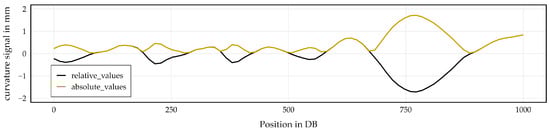
Figure 2. The curvature signal around the crossing nose is broken down into 500 DB window, with the signal before and after the crossing nose area. The raw curvature signal is shown in black and the absolute values in yellow.

The resulting cumulative curves are then compared to detect systematic deviations between runs. Figure 3 shows an example of a turnout, illustrating the cumulative summation of the absolute values from the previous Figure 2. Each color represents a distinct measurement run. This plot includes six measurement runs conducted between 2019 and 2021. As in the previous Figure 2, a length of 1000 DB around the crossing nose area is highlighted. The values at the end of the cumulative curves are subsequently employed to identify runs that were not performed along the main direction of travel.

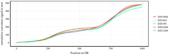
Figure 3. The cumulative summation of the absolute curvature values from an arbitrary turnout. Each color represents a different measurement run (there were six runs between 2019 and 2021). The area around the crossing nose with 1000 DB is shown, and the cumulative values at the end are used to identify runs outside the main direction of travel.

The second approach is cross-correlation, which we primarily use for outlier detection rather than synchronization. One signal is shifted relative to the other, and similarity is computed at each step, typically using a sliding scalar product or the Pearson correlation coefficient. The Pearson coefficient measures the linear relationship between two signals. Values close to +1 indicate a strong positive correlation, values near −1 indicate a strong negative correlation, and values around 0 indicate no linear relationship. The resulting correlation function (correlation coefficient as a function of applied signal shift) reflects the degree of match at different relative positions, and the maximum correlation identifies the offset at which the signals are most similar. Runs that fail to reach a sufficient correlation level of xy are identified as outliers [29].

2.4. Synchronization and Evaluation Method

Figure 4 shows a 250 m segment of the turnout window, highlighting the longitudinal offset between measurement runs before any synchronization is applied. The x-axis represents mileage in data breaks (DB), where one DB corresponds to 25 cm. To improve clarity, only 1000 DB are displayed, which correspond to 250 m and sufficiently cover the turnout area. The crossing nose is positioned at 2000 DB to ensure the entire turnout is captured within this segment. Since the longest turnouts in Austria are approximately 136 m, this selection is adequate.

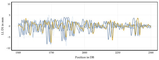
Figure 4. Initial longitudinal level D1 signals of the left rail in a 250 m turnout segment. A subset of the measurement runs is shown in different colors to illustrate variations before synchronization is applied. The crossing nose is located at 2000 DB; one DB corresponds to 25 cm.

The longitudinal level D1 signal of the left rail is plotted because it serves as the primary reference for subsequent synchronization; all other signals will be aligned accordingly. A subset of measurement runs is displayed in different colors to clearly illustrate the variations between runs. These colors are illustrative and will be explained in the synchronization process.

This overview highlights the differences in longitudinal level signals and emphasizes the necessity of subsequent pre-synchronization and fine-tuning procedures to achieve precise synchronization. Please note that the following figures illustrate a representative example and are not intended to be generally applicable to all turnouts.

The synchronization process begins with pre-synchronization of the measurement runs based on the mileage signal. The location of the measurement vehicle is determined by a combination of differential GPS and distance traveled along the track obtained by wheel revolutions. Positioning information is stored within the mileage signal. The median mileage of each run is calculated and used as the initial reference point. Then, a reference mileage series is generated at consistent 25 cm intervals along the turnout section. This provides the framework for signal synchronization. The difference between the median mileage and each measurement point is computed and the resulting offset is applied to all signals within the run. Measurement runs that show significant deviation after this adjustment are removed to ensure only consistent, reliable data proceed to the fine synchronization stage.

The pre-synchronization results are presented in Figure 5 using the same setup as in Figure 4. It demonstrates a 250 m segment of the turnout window. Although pre-synchronization reduces offsets between runs overall, it is insufficient for precise synchronization. The peaks of the different runs are grouped within a similar range (approximately 30 DB in this specific example) but are not perfectly synchronized. This underscores the need for additional synchronization steps to accurately synchronize all measurement signals.

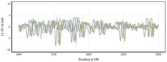
Figure 5. The longitudinal level D1 signal of the left rail in a 250 m turnout window. Pre-synchronized measurement runs are displayed in different colors to illustrate the initial synchronization based on mileage. The crossing nose is at 2000 DB; offsets between runs indicate the need for further synchronization.

After pre-synchronization, any measurement run that do not follow the main direction of travel of the examined turnout is identified using the curvature signal and excluded. The main direction of travel is defined as the branch that is mainly traversed in each turnout. This is usually the straight (through) branch, but can be the diverging branch in some cases. For instance, if the main branch is straight and a measurement run follows the diverging path, the curvature signal will exhibit a characteristic curve shape corresponding to the bending of the turnout, which can be detected. Each remaining run is then synchronized relative to the most recent valid run using the Euclidean distance method. The runs are then converted into a cumulative sum for outlier detection, as illustrated in Figure 3. The first (Q1) and third (Q3) quartiles of the cumulative sum values are calculated, and the interquartile range (IQR) is used to define the upper and lower thresholds (Q3 + 1.5 × IQR and Q1 − 1.5 × IQR, respectively). Runs outside these thresholds are classified as outliers and removed. All excluded runs are stored separately for traceability.

Next, the measurement runs are divided into blocks based on significant differences in signal amplitude, which indicate executed maintenance activity. To identify these changes, a 100 m window around the crossing nose is analyzed for each run. Within this section, the standard deviation of the signal is calculated to quantify amplitude variations. Then, the difference between each run and its two predecessors is determined. A maintenance event is assumed if the first difference is below 0.8 mm and the second difference exceeds 1 mm. This approach groups the measurement runs into blocks with consistent signal characteristics over time. Each significant change, typically due to maintenance, marks the beginning of a new block. Figure 6 schematically illustrates this step, where measurement runs from different blocks are color-coded: yellow represents runs from an older block, and blue represents runs from a more recent block.

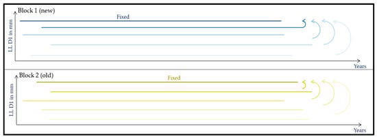
Figure 6. Schematic representation of block partitioning. Block 1 corresponds to the most recent block, and Block 2 corresponds to the oldest. In this step, the latest measurement run within a block serves as the reference, and all other runs are synchronized to it.

Within each block, the signals are synchronized relative to one another using the Euclidean distance method described in Section 2.3. This synchronization is based on the longitudinal level of the left rail, which serves as the primary reference signal. All other signals are shifted by the same offset determined for this reference signal to maintain consistent synchronization. The most recent measurement run of the block serves as the reference. A block represents a subset of measurement runs over time that exhibit stable signal behavior. Synchronization is performed in three stages to progressively increase precision—from global synchronization to local fine synchronization:

• Coarse synchronization: The entire signal is shifted as a whole, with a maximum displacement of 101 m allowed.
• Focused synchronization: The signal is conceptually divided into three equal parts, and the Euclidean distance is computed for the central 333 m around the crossing nose. Based on this, the signal is adjusted with a maximum displacement of 10 m.
• Local adjustment: The signal is divided into consecutive 200 m segments, each of which is adjusted individually with a maximum shift of 0.25 m to correct for local stretching or compression.

Once these adjustments have been made, the length of the signal is verified. Any signals that have been shortened to the point that there is insufficient data are excluded from further synchronization.

The results of applying the block-based synchronization procedure are shown in Figure 7. The displayed segment corresponds to the same 250 m turnout section shown in Figure 4 and Figure 5. Within this partitioning, all measurement runs of a single block are represented by different shades of blue. The darkest blue line indicates the most recent run of the block. The yellow line corresponds to the earliest run of the subsequent block. The blue signals are well-synchronized, demonstrating the effectiveness of the three-stage synchronization procedure within a block. This procedure progressively refines synchronization from coarse to local adjustments. In contrast, in this specific example, the yellow line from the subsequent block remains offset by approximately 30 DB, indicating that inter-block synchronization has not yet occurred. This confirms that the method successfully synchronizes runs within a block while preserving the distinction between different blocks for subsequent processing.

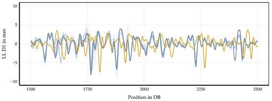
Figure 7. Synchronization of measurement runs within a single block (blue lines) and the earliest run of the subsequent block (yellow line) in a 250 m turnout segment. The three-stage procedure synchronizes signals within the block while maintaining a visible inter-block offset of approximately 30 DB.

The synchronized blocks are then aligned relative to each other using the Euclidean distance method to ensure chronological consistency across all maintenance periods. During this process, each block is treated as a single unit and shifted as a whole without further internal segmentation. The most recent block serves as the reference, and the earlier blocks are sequentially synchronized, allowing a maximum displacement of 101 m. Only the middle third (333 m) of each block is considered when calculating the maximum displacement. For inter-block synchronization, the second-oldest and second-newest runs of each block are used, excluding the oldest and newest runs, which tend to show the highest amplitude differences. This procedure is illustrated schematically in Figure 8. The figure shows the blocks after synchronization, with the two reference measurement runs of each block highlighted in green. The reference of the most recent block remains fixed while the references of the preceding blocks are synchronized to it. All other measurement runs within each block are synchronized accordingly, providing a visual overview of how inter-block synchronization is achieved and ensuring consistency across the entire dataset.

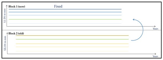
Figure 8. Schematic illustration of the next step after Figure 6, showing the blocks after synchronization. The green lines highlight the reference measurement runs of each block. The reference in Block 1 remains fixed while the reference in Block 2 is synchronized with the first. All other measurement runs within each block are synchronized accordingly.

Synchronization of blocks relative to each other is illustrated in Figure 9. The 250 m turnout segment is shown as it was in Figure 4, Figure 5 and Figure 7. At this stage, all blocks are treated as single units and synchronized chronologically using the Euclidean distance method. The blue lines represent runs from a single block, while the yellow line corresponds to a run from a different block. After inter-block synchronization, the yellow line aligns perfectly with the blue lines. This eliminates the previous offset in the peaks and shows that the signals are now synchronized optimally. The most recent block serves as the reference, so all synchronizations are relative to it. This is evident in the overlay of the signals. This confirms that the inter-block synchronization procedure successfully brings all blocks into consistent chronological order while preserving the integrity of each block.

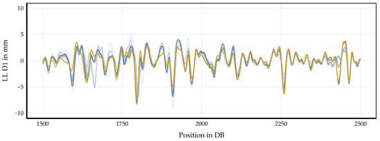
Figure 9. Inter-block synchronization of measurement runs in a 250 m turnout segment. The blue lines represent runs from a single block, while the yellow line corresponds to a run from a different block. The signals are synchronized relative to the most recent block, resulting in an optimal overlay of all amplitudes.

Finally, cross-correlation analysis is applied to detect any remaining misaligned or faulty runs using the longitudinal level and mileage signals. Each measurement run is correlated with all the others, and a linear cross-correlation coefficient is calculated for each pair. Measurement runs whose maximum correlation with all the others falls below 0.275 are considered misaligned or unreliable and are removed from the main dataset. To ensure full traceability, these excluded measurement runs are stored separately and can be reviewed or analyzed later.

This structured, multi-stage approach generates temporally consistent, turnout-specific datasets that are resistant to measurement artifacts. The resulting synchronized data provide a reliable basis for calculating quality indices, enabling accurate condition assessments and predictive maintenance planning.

After establishing a robust and systematic methodology for signal synchronization and pre-processing, it is important to explain how the proposed approach differs from existing synchronization methods. The key difference is the introduction of the block-partitioning strategy, which has not been used before to improve synchronization accuracy in turnout areas. Earlier studies often require manual adjustments, particularly in complex turnout sections where signal characteristics change abruptly. The proposed method, however, enables fully automated synchronization tailored to these conditions. Synchronization on open track is generally easier due to more homogeneous signal behavior. However, this assumption does not apply to turnout areas. The proposed framework addresses this gap by achieving full automation in turnout monitoring without manual intervention.

After developing this methodology, the final step is to evaluate the performance of the automated synchronization process. The following chapter thoroughly evaluates the synchronization framework by addressing the validity of the measurement runs, the computational efficiency of the process, and the practical effectiveness of signal synchronization in turnout areas.

3. Evaluation of the Automated Synchronizations Framework

The performance of the automated synchronization framework is evaluated from multiple perspectives. First, the validity of the measurement runs is assessed to determine if the synchronized data accurately represent the track geometry and turnout conditions. This evaluation lays the groundwork for subsequent analyses of computational performance and the practical applicability of the synchronization approach.

3.1. Assessment of Measurement Run Validity

The analysis evaluated the proportion of valid measurement runs across the 109 turnouts investigated. As Figure 10a shows, about 73% of all measurement runs were successfully synchronized and classified as valid. Initially, 19% of runs were excluded because the track-recording vehicle did not pass through the turnout window. A further 7% were removed due to excessive longitudinal shifts during pre-synchronization, resulting in incomplete coverage of the one-kilometer analysis section. Fewer than 1% of the measurement runs were excluded because the track- recording vehicle did not traverse the turnout in the main traffic direction. Overall, these results indicate that approximately three-quarters of the measurement runs were suitable for use without additional correction. This demonstrates the high baseline reliability of the proposed method.

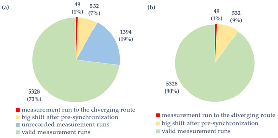
Figure 10. (a) Proportion of valid measurement runs after applying all evaluation criteria, and (b) proportion of valid measurement runs that are important for synchronization.

Figure 10b illustrates the effect of the synchronization process itself, excluding unrecorded runs that were never included in the synchronization procedure. Within this subset, only around 10% of measurement runs were rejected, mainly due to insufficient run length after pre-synchronization. A smaller part of the runs resulted from the track-recording vehicle not traversing the turnout in the main traffic direction. Consequently, nearly 90% of the processed runs were successfully synchronized and validated, confirming the efficiency and robustness of the automated framework. The low proportion of discarded runs, which was achieved without manual adjustment, highlights the reliability and scalability of the approach for large-scale turnout analysis.

3.2. Computational Performance

In addition to improving data quality, the automated procedure offers significant advantages in terms of processing efficiency. Currently, complete turnout synchronization takes only a few minutes, depending on the volume of data. Previous approaches were significantly more time-intensive and relied heavily on manual interaction. Earlier methods required filtering, entering parameters, and correcting misaligned runs for each turnout, making large-scale processing impractical. By eliminating these manual steps, the proposed approach improves computational efficiency and scalability, enabling the automated analysis of extensive measurement datasets.

4. Results

The synchronization framework that we developed in this research is the main methodological outcome and forms the basis for all subsequent evaluations in turnouts. It integrates data preprocessing, direction-based filtering, amplitude-based block partitioning, and multi-stage signal synchronization into a consistent, reproducible process. This structured approach ensures that measurement runs from different time periods are spatially and temporally synchronized with high precision. This enables a consistent evaluation of turnout geometry evolution over time.

Figure 11 provides a schematic overview of the entire synchronization process, summarizing the essential stages from data preparation to final validation. The process begins with extracting track geometry measurement data and turnout metadata. Then, mileage-based pre-synchronization and direction filtering using curvature signals are performed. Next, measurement runs are divided into blocks based on amplitude variations indicating maintenance interventions. Within each block, three-stage synchronization comprising coarse, focused, and local synchronizations ensures precise spatial correspondence among measurement runs. Then, inter-block synchronization establishes chronological consistency across different maintenance periods. Finally, a cross-correlation validation step detects and removes misaligned or unreliable runs.

Figure 11. Overview of the multi-stage synchronization workflow. The process begins with data acquisition and rough pre-synchronization based on mileage references. This is followed by direction filtering and block partitioning. Within each block, runs are synchronized in three stages using the Euclidean distance method. Inter-block synchronization then ensures chronological consistency across maintenance periods. Finally, cross-correlation validation detects and removes any remaining misaligned or unreliable runs.

In summary, the workflow in Figure 11 encapsulates the complete synchronization methodology, demonstrating how raw, heterogeneous measurement data are transformed into temporally consistent, turnout-specific datasets suitable for advanced condition assessments and predictive maintenance applications.

5. Discussion

This study investigated whether using an automated synchronization procedure for measurement runs could improve signal positioning accuracy along the turnout and reduce the amount of manual work needed for data preparation. The proposed approach synchronizes measurement signals consistently and establishes a robust foundation for evaluating conditions and conducting long-term monitoring. The results demonstrate the method’s efficiency, scalability, and ability to process large datasets without manual intervention. Consequently, infrastructure operators can assess turnout conditions more accurately and support data-driven, predictive maintenance strategies. This is particularly important in a broader sense because synchronized and reliable measurement data form the basis for all subsequent analyses, providing critical input that enables informed decision-making in life-cycle management and optimizes the allocation of maintenance resources, thereby contributing to the resilience of railway infrastructure.

These findings align with previous research conducted at Graz University of Technology, where various turnout quality indicators have been developed [7,30]. The automated procedure ensures precise signal synchronization, enhancing the reliability of these indicators and facilitating continuous monitoring by infrastructure managers. Compared to conventional methods that rely on extensive manual processing and correction, the proposed framework significantly advances automation, scalability, and consistency of results.

Beyond the specific results, the main benefit of this research lies in providing a standardized, fully automated synchronization process that others working with similar measurement data can adopt. Synchronizing such data is a necessary step for anyone conducting track monitoring, yet it is often time-consuming and resource-intensive. This process also facilitates more efficient and reproducible data preparation and analysis, supporting further research in railway infrastructure monitoring.

Despite these advantages, certain limitations remain. Specific parameters, such as half-gauge values, could not be integrated into the synchronization process because these signals were not consistently available during the analyzed measurement campaigns. Additionally, since the current method only performs relative synchronization, the resulting datasets are not linked to absolute track positions (mileage). This may limit comparability across different datasets or campaigns. Future work should therefore address absolute synchronization. One way to achieve this would be through georeferencing, which currently requires manually identifying the turnout position within the signal. These developments would improve cross-dataset comparability and expand the applicability of the proposed approach.

References

- Kollment, W.; O’Leary, P.; Harker, M.; Osberger, U.; Eck, S. Towards condition monitoring of railway points: Instrumentation, measurement and signal processing. In Proceedings of the 2016 IEEE International Instrumentation and Measurement Technology Conference Proceedings, Taipei, Taiwan, 23–26 May 2016; pp. 1–6. [Google Scholar] [CrossRef]
- Esveld, C. Modern Railway Track, 2nd ed.; MRT-Productions: Zaltbommel, The Netherlands, 2001. [Google Scholar]
- Kawaguchi, A.; Miwa, M.; Terada, K. Actual Data Analysis of Alignment Irregularity Growth and its Prediction Model. Q. Rep. RTRI 2005, 46, 262–268. [Google Scholar] [CrossRef]
- Peng, F.; Kang, S.; Li, X.; Ouyang, Y.; Somani, K.; Acharya, D. A Heuristic Approach to the Railroad Track Maintenance Scheduling Problem: A heuristic approach to the railroad track maintenance scheduling problem. Comput.-Aided Civ. Infrastruct. Eng. 2011, 26, 129–145. [Google Scholar] [CrossRef]
- Veit, P.; Marschnig, S. Sustainability in Track: A Precondition for High Speed Traffic. In 2010 Joint Rail Conference; ASMEDC: Urbana, IL, USA, 2010; Volume 2, pp. 349–355. [Google Scholar] [CrossRef]
- Xu, P.; Sun, Q.; Liu, R.; Wang, F. A short-range prediction model for track quality index. Proc. Inst. Mech. Eng. Part F J. Rail Rapid Transit 2011, 225, 277–285. [Google Scholar] [CrossRef]
- Loidolt, M. Integration of Short-Wave Effects into Asset Management of Railway Infrastructure. Doctoral Thesis, Graz University of Technology, Graz, Austria, 2024. [Google Scholar]
- Fellinger, M. Sustainable Asset Management for Turnouts; Verlag der Technischen Universität Graz: Graz, Austria, 2020. [Google Scholar] [CrossRef]
- Wang, Y.; Wang, P.; Wang, X.; Liu, X. Position synchronization for track geometry inspection data via big-data fusion and incremental learning. Transp. Res. Part C Emerg. Technol. 2018, 93, 544–565. [Google Scholar] [CrossRef]
- Weston, P.; Roberts, C.; Yeo, G.; Stewart, E. Perspectives on railway track geometry condition monitoring from in-service railway vehicles. Veh. Syst. Dyn. 2015, 53, 1063–1091. [Google Scholar] [CrossRef]
- Xu, P.; Sun, Q.-X.; Liu, R.-K.; Wang, F.-T. Key Equipment Identification model for correcting milepost errors of track geometry data from track inspection cars. Transp. Res. Part C Emerg. Technol. 2013, 35, 85–103. [Google Scholar] [CrossRef]
- Saab, S.S.; Nasr, G.E.; Badr, E.A. Compensation of axle-generator errors due to wheel slip and slide. IEEE Trans. Veh. Technol. 2002, 51, 577–587. [Google Scholar] [CrossRef]
- Khosravi, M.; Soleimanmeigouni, I.; Ahmadi, A.; Nissen, A. Reducing the positional errors of railway track geometry measurements using alignment methods: A comparative case study. Measurement 2021, 178, 109383. [Google Scholar] [CrossRef]
- Xu, P.; Sun, Q.; Liu, R.; Souleyrette, R.R. Optimal Match Method for Milepoint Postprocessing of Track Condition Data from Subway Track Geometry Cars. J. Transp. Eng. 2016, 142, 04016028. [Google Scholar] [CrossRef]
- Wang, M.; Xiao, Y.; Li, W.; Zhao, H.; Hua, W.; Jiang, Y. Characterizing Particle-Scale Acceleration of Mud-Pumping Ballast Bed of Heavy-Haul Railway Subjected to Maintenance Operations. Sensors 2022, 22, 6177. [Google Scholar] [CrossRef]
- Steuer, M.; Krzykawski, M.; Simiński, D.; Chema, W.; Burdzik, R. Train detection methods as the foundation of positioning systems of railroad traffic control. Diagnostyka 2023, 24, 1–7. [Google Scholar] [CrossRef]
- Fikejz, J.; Kavička, A. RegioRail—GNSS Train-Positioning System for Automatic Indications of Crisis Traffic Situations on Regional Rail Lines. Appl. Sci. 2022, 12, 5797. [Google Scholar] [CrossRef]
- Lau, A.; Fan, H.; Yan, H. A Schematic Plan for Train Position Identification Using Digital Twin and Positioning Sensors. In Transport Transitions: Advancing Sustainable and Inclusive Mobility; McNally, C., Carroll, P., Martinez-Pastor, B., Ghosh, B., Efthymiou, M., Valantasis-Kanellos, N., Eds.; Springer Nature: Cham, Switzerland, 2026; pp. 212–218. [Google Scholar] [CrossRef]
- Vu, A.; Ramanandan, A.; Chen, A.; Farrell, J.A.; Barth, M. Real-Time Computer Vision/DGPS-Aided Inertial Navigation System for Lane-Level Vehicle Navigation. IEEE Trans. Intell. Transp. Syst. 2012, 13, 899–913. [Google Scholar] [CrossRef]
- Ndoye, M.; Barker, A.M.; Krogmeier, J.V.; Bullock, D.M. A Recursive Multiscale Correlation-Averaging Algorithm for an Automated Distributed Road-Condition-Monitoring System. IEEE Trans. Intell. Transp. Syst. 2011, 12, 795–808. [Google Scholar] [CrossRef]
- Selig, E.T.; Cardillo, G.M.; Stephens, E.; Smith, A. Analyzing and forecasting railway data using linear data analysis. In Computers in Railways XI: Computer System Design and Operation in the Railway and Other Transit Systems; WIT Press: Toledo, Spain, 2008; pp. 25–34. [Google Scholar] [CrossRef]
- Sakoe, H.; Chiba, S. Dynamic programming algorithm optimization for spoken word recognition. IEEE Trans. Acoust. Speech Signal Process. 1978, 26, 43–49. [Google Scholar] [CrossRef]
- Tomasi, G.; Van Den Berg, F.; Andersson, C. Correlation optimized warping and dynamic time warping as preprocessing methods for chromatographic data. J. Chemom. 2004, 18, 231–241. [Google Scholar] [CrossRef]
- Nielsen, N.-P.V.; Carstensen, J.M.; Smedsgaard, J. Aligning of single and multiple wavelength chromatographic profiles for chemometric data analysis using correlation optimised warping. J. Chromatogr. A 1998, 805, 17–35. [Google Scholar] [CrossRef]
- Jiang, W.; Zhang, Z.-M.; Yun, Y.; Zhan, D.-J.; Zheng, Y.-B.; Liang, Y.-Z.; Yang, Z.Y.; Yu, L. Comparisons of Five Algorithms for Chromatogram Alignment. Chromatographia 2013, 76, 1067–1078. [Google Scholar] [CrossRef]
- Ji, Y.; Huang, Y.; Yang, M.; Leng, H.; Ren, L.; Liu, H.; Chen, Y. Physics-informed deep learning for virtual rail train trajectory following control. Reliab. Eng. Syst. Saf. 2025, 261, 111092. [Google Scholar] [CrossRef]
- Offenbacher, S. Effective Railway Track Tamping: Evaluating Short-Term and Long-Term Impacts on Track Geometry and Monitoring Ballast Condition. Doctoral Thesis, Graz University of Technology, Graz, Austria, 2025. [Google Scholar]
- ÖNORM EN 13848-1:2018; Railway Applications–Track–Track Geometry Quality–Part 1: Characterization of Track Geometry. Austrian Standards International (ASI): Vienna, Austria, 2018.
- Hovad, E.; Thyregod, C.; Andersen, J.F.; Lyndgaard, C.B.; Spooner, M.P.; Rodrigues, A.F.D.S.; Ersbøll, B.K. The effect of driving direction on spatially aligned track recording car measurements in turnouts. Int. J. Rail Transp. 2020, 8, 234–248. [Google Scholar] [CrossRef]
- Loidolt, M.; Egger, J.; Korenjak, A.K. Data-Driven Condition Monitoring of Fixed-Turnout Frogs Using Standard Track Recording Car Measurements. Appl. Sci. 2025, 15, 11122. [Google Scholar] [CrossRef]
Disclaimer/Publisher’s Note: The statements, opinions and data contained in all publications are solely those of the individual author(s) and contributor(s) and not of MDPI and/or the editor(s). MDPI and/or the editor(s) disclaim responsibility for any injury to people or property resulting from any ideas, methods, instructions or products referred to in the content. |
© 2025 by the authors. Licensee MDPI, Basel, Switzerland. This article is an open access article distributed under the terms and conditions of the Creative Commons Attribution (CC BY) license.