Optimum Geometries for Wireless Power Transfer Between an Oblong Coil and a Rectangular Coil

Featured Application

Dynamic Inductive Wireless Power Transfer to Electric Vehicles.

Abstract

The geometry of the coils in a magnetic link and their relative position are crucial for increasing their mutual inductance, which is important for obtaining a higher induced voltage, transferred power, and electrical efficiency. General design guidelines found in the literature point to an increase in mutual inductance by making the coils similar in shape, positioning them as close as possible, and using high-permeability soft-cores to concentrate the flux between them. But these recommendations are often difficult to follow in dynamic inductive wireless power transfer (DIWPT) configurations for vehicular applications. This is mostly due to the necessity of a mechanical clearance between the lane and the vehicle assembly, which creates an “air gap”. Also, unless tracks are used, the lateral movement of a vehicle over a primary coil potentially causes a variation in the induced voltage, which is not adequate to energize the powertrain. Considering these intrinsic problems of DIWPT applications, we developed a few theorems that might facilitate some optimum designs, in the case where rectangular secondary coils are used over oblong primary coils, for two different design targets: (i) maximum induced voltage on the secondary coil and (ii) better insensitivity to the vehicle lateral misalignment on the inductive lane.

1. Introduction

The simplicity of the design of dynamic inductive wireless power transfer (DIWPT) with oblong primary coil configurations, which had long ago been invented [1,2], was rediscovered [3,4,5,6] in the late 20th century, as a result of a growing interest in electric vehicles (EVs). After 2010, the quest for sustainable EV transportation motivated the use of dynamic inductive wireless power transfer (DIWPT) for automotive applications in the design, implementation, and testing of more advanced and practical prototypes, for instance, the OLEV Bus from the Korea Advanced Institute of Science & Technology (KAIST) [7,8] and Section 9.4 of [9], which, by its innovative conception and extensive public demonstration, can be considered disruptive.

While researchers at KAIST were searching for high-end, on-the-road recharging of electric buses, it was the smaller conceptual demonstration prototype developed at NISSAN, in Japan [10], that most attracted our attention, for its simplicity, and for handling lower power levels, around 1 kW, more adequate for lightweight electric vehicles. So, inspired by the work of all these researchers, we set the target of implementing an inductive lane for electrically assisted bicycles and other similar cycles [11].

Our prototype was then devised for the continuous operation of a PEDELEC-type bicycle, which, according to guidelines [12], could only receive up to 250 W of electric assistance to the powertrain. The lane was capable of transferring the full power limit of 250 W inside a 27 cm wide corridor, center-aligned with the bike lane, but more, 400 W, over a 20 cm wide corridor within it. A standard bike was specially adapted to dynamically harvest energy from this inductive lane. Depending on the lateral misalignment of the bike within the 27 cm wide central corridor of the lane, up to 150 W of excess power could be harvested over the 250 W limit. This was enough to store short-term energy that could allow the smooth activation of the powertrain during the transit of the bike between neighbor primary coils lying along the lane.

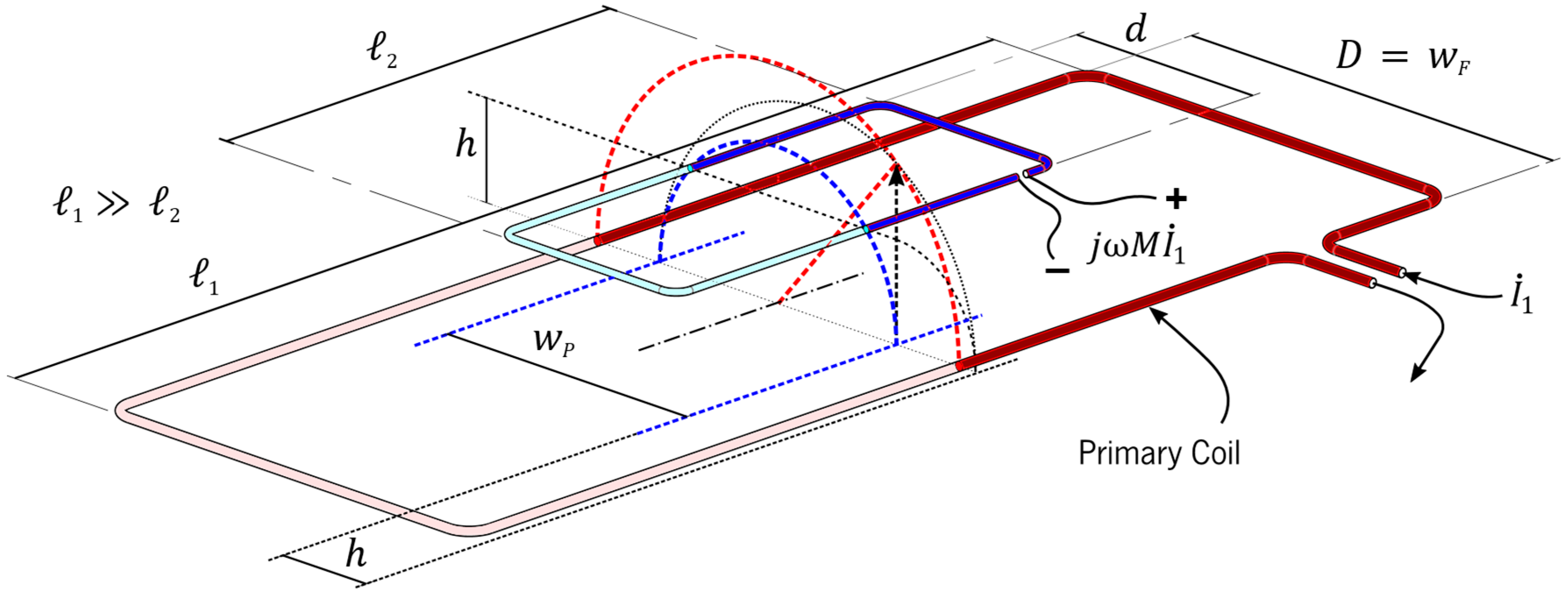
The geometric configuration of the protype that made this possible was derived by installing an as large as possible secondary coil, wound around its rear wheel and fixed to the frame of the bike as close as possible to the lane. This was carried out in such a way that this secondary coil would not mechanically interfere with the normal maneuvering of the bike, nor with the pedaling action of the rider.

Targeting a solution with a reduced electronic component count (per unit of length) on the lane side, the use of oblong primary coils seemed to be the most natural design paradigm to be adopted. It was then necessary to design the cross-section of the magnetic link, due to the intrinsic symmetry of the configuration.

After gross estimations, we searched, by experimentation, for a set of combinations of primary current values and relative sizes and positions of the coils that would successfully yield the nominal 36VDC required by the powertrain, at a chosen operation frequency. The onboard circuitry was set to rectify the induced voltage, filter it, and, finally, regulate it by the use of a step-down DC-DC converter.

In the tests, as intuitively expected, it became apparent that for a given primary current and a fixed distance imposed between the planes containing the primary and secondary coils, there would be an optimum width for the oblong primary coil that would maximize the induced voltage on the secondary coil. This condition would lead to the maximum possible power to be extracted from the secondary coil, if impedance matching and other circuit parameters were carefully adjusted. Conversely, this same configuration would also minimize the primary current that was necessary to obtain some given desired induced voltage or power level on the powertrain, thus diminishing losses on the primary winding and favoring an improved electric efficiency of the system.

During the continuation of our investigation, almost immediately after our first publication was released, additional tests seemed to indicate that, when implemented by single-turn coils, the induced voltage would be maximized when the coils were under center alignment conditions and the centers of the primary coil wiring cross-sections formed the diameter of a semi-circle approximately containing the centers of the wiring cross-sections of the secondary coil as well. However, our interest at that time was redirected to the design of a technique for automatically sensing the presence of the bike over the primary coil to enable its inductive field [13], and this interesting observation was momentarily forgotten. By the end of 2017, the simple mathematics justifying our results (Theorem 2, Section 3.2) was finally established, but it was initially perceived as a mere curiosity, and kept undocumented until it was included as part of the thesis work of the first author [14], remaining otherwise unpublished.

The recent accomplishment of several large-scale DIWPT prototypes and pilot installations, such as the FABRIC project [15,16] and the Smartroad Gotland project, in Sweden [17], brought a whole new interest in the subject. But at the same time, they revealed the relatively much higher costs involved in the deployment of this technology with respect to any other conductive road electrification techniques [18]. However, it is our impression that, when lightweight vehicles are considered, instead of standard, heavier road vehicles, the decrease in the required power levels can make the system costs drop significantly. On one hand, this is because the components used in lower-power circuits are less expensive than those used in higher-power ones. On the other hand, when dealing with lightweight, low-power vehicles, lower electric efficiencies can be better tolerated, and then oblong primary coils (those that are much longer than wider), also much longer than the secondary coils, can be used, despite the lower magnetic coupling coefficients obtained. The consequence is that DIWPT for lightweight EVs could also require much fewer inverter modules per kilometer, helping the maintainability and further decreasing the overall costs.

Considering these possible future DIWPT systems for lightweight EV applications, we reunite in this paper some theorems that will help the design of inductive lanes constituted by oblong primary coils. The theorems indicate the optimum dimensions of the other coil in a magnetic link, which can be either the primary (transmitter) coil or the secondary (receiver) coil. Optimality here refers to two distinct possible design goals: (i) obtaining the maximum open-circuit voltage induced on the secondary coil, or (ii) obtaining the maximally flat response for the open-circuit induced voltage, as the coils are laterally displaced from the center alignment position.

Although all the theorems were derived under the hypothetical situation of filamentary (circular with zero diameter) wires and single-turn coils, we infer that the width estimation given by these theorems will reasonably approximate the actual value of the respective optimum width in a real system if (i) the wire diameters are much smaller than both the coil widths and the distance between coils, thus resulting in a relatively large distance between any two conductors in different coils, and (ii) we use the abstraction of replacing the multiple turns of a coil winding by the same number of turns coinciding, but electrically isolated, on the same support line in a suitably interpolated position. This approximation has been actually experimentally verified for the case of Theorem 1 (general expression for induced voltage) and Theorem 2 (optimum primary coil width that maximizes the induced voltage on given rectangular secondary coil). The experimental verification of Theorems 3 to 5 are left for future work.

2. Wireless Power Transfer

2.1. A Simple Circuit Model for Wireless Power Transfer

When submitted to sinusoidal oscillations of a frequency $f_0$ that is low enough so that the radiated power is negligible, the magnetic coupling can be modeled in terms of phasors by ideal linear circuit components, as shown in Figure 1.

Figure 1. Two non-radiating magnetically coupled coils (a) and their simplified circuit model (b).

In this model, $\omega =2\pi f_0$, and $M$ is the mutual inductance between the two coils, with self-inductances $L_1$ and $L_2$. $R_1$ and $R_2$ are the resistances of the primary and secondary coil windings and depend, among other factors, on both skin and proximity effects. For any fixed frequency of operation, $f_0$, these parameters should be recalculated so that the model can still conserve its linearity. In this manner, in a sinusoidal regimen, with no radiation assumed for the magnetic coupling, the power transferred from Coil 1 to Coil 2 is given by the phasor ${\dot{S}}_{\mathrm{1,2}}$:

$${\dot{S}}_{\mathrm{1,2}}\mathrm{}=\mathrm{}\mathrm{}{\dot{V}}_{M_1}{\dot{I}}_1^{\ast }\mathrm{}\mathrm{}=\mathrm{}\mathrm{}\mathrm{}j\omega M{\dot{I}}_1^{\ast }{\dot{I}}_2\mathrm{},$$

(1)

where for $i∊ \left\{1, 2\right\}$, ${\dot{V}}_{M_{\mathrm{I}}}$ and ${\dot{I}}_{\mathrm{I}}$ are the phasors representing, respectively, the voltage across the dependent voltage source and the current flowing on side $i$ of the magnetic coupling.

Under the hypothesis of a compensated secondary, where the effect of the impedance of the self-inductance $L_2$ is essentially canceled, and a linear resistive load $R_{\mathrm{L}}$, ${\dot{I}}_2$ will be proportional to the induced voltage on the secondary coil, $j\omega M{\dot{I}}_1$, so the transferred power ${\dot{S}}_{\mathrm{1,2}}$ will be expressed by

$${\dot{S}}_{\mathrm{1,2}}\mathrm{}=\mathrm{}\mathrm{}{\dot{V}}_{M_1}{\dot{I}}_1^{\ast }\mathrm{}\mathrm{}=\mathrm{}\mathrm{}\left(\mathrm{}j\omega M{\dot{I}}_{1\mathrm{}}^{\ast }\right)\mathrm{}\left(j\alpha \omega M{\dot{I}}_1\right)=\alpha {\left(\omega M\right)}^2{\dot{I}}_1{\dot{I}}_{1\mathrm{}}^{\ast }=\alpha {\left|\omega M{\dot{I}}_1\right|}^2$$

(2)

where $\alpha >0$.

So, as expected, the transferred power will be proportional to the square of the modulus of the voltage induced on the secondary coil by the primary current ${\dot{I}}_1$, which will be proportional to the product of the frequency of operation, the mutual inductance between the coils, and the primary current itself.

In this way, under the same circuit conditions of the secondary coil and oversimplifying the real magnetic links to the simple model of Figure 1, in order to increase the transferred power, it is necessary to increase either the frequency of oscillation, $f_0$, the mutual inductance, $M$, or the amplitude of the primary current, ${\dot{I}}_1$. For a fixed frequency $f_0$, and fixed a maximum primary current ${\dot{I}}_1$ (a physical limitation of the primary coil or the circuit driving it), the maximum available power transfer will be obtained when $M$ is also maximized.

2.2. Mutual Inductance of a Magnetic Link in DIWPT Configurations

A calculation tool for the mutual inductance, $M$, between two filamentary coils with windings modeled by curves ${\mathrm{k}}_1$ and ${\mathrm{k}}_2$ in ${\mathbb{R}}^3$ was established by Newmann [19,20], and it is now expressed in the International System of Units by

$$M\mathrm{}=\mathrm{}\mathrm{}{\displaystyle \frac{\mu }{4\pi }}\underset{{\mathrm{k}}_1}{\oint }\underset{{\mathrm{k}}_2}{\oint }{\displaystyle \frac{\overrightarrow{d{\mathcal{l}}_1}.\overrightarrow{d{\mathcal{l}}_2}}{r}},$$

(3)

where $r$ is the distance between the points of ${\mathrm{k}}_1$ and ${\mathrm{k}}_2$, for which the infinitesimal oriented elements $\overrightarrow{d{\mathcal{l}}_1}$ and $\overrightarrow{d{\mathcal{l}}_2}$ are, respectively, considered, and $\mu$ is magnetic permeability of the medium in which the coils are immersed. Thus, $M$ is purely dependent on the geometry of the magnetic link.

For real, non-filamentary coils, the distribution of the current density inside the conductors along each cross-section has to be considered, and a dependence of $M$ on the inducing frequency starts to show when the frequency itself is high enough to make the skin depth in the conductors become comparable to or smaller than the diameter of the wires used in the coil windings. But, in many practical cases, designers tend to avoid this condition to reduce winding losses, and a good estimate of the mutual inductance can still be provided by (3).

But (3) is usually difficult to solve analytically. When some closed-form expression for the mutual inductance is found, often it is not a simple one, preventing intuition from building up in the designer. In fact, most of the design cases can be exclusively accomplished by numeric computation. This has been particularly observed when dealing with “short” coils, that is, coils of about the same size, where each of them also has its a longer dimension of the same magnitude as its shorter dimension. Notably, in this class of coils, formulation and precise computation methods for self- and mutual inductances have been determined for circular [21,22,23,24] and rectangular shapes [25] Chapter 8, [26,27,28,29,30], and even for some hybrid variants [31]. Short coils of other shapes have also been studied, such as the double “D” coils [32], which, in addition to the good power transfer capabilities of other short coils, exhibit a diminished fluctuation of the induced voltage and the resulting transferred power (“power pulsation”) as the vehicle moves along its path.

The electric losses in oblong primary coils, for a given alternate current, tend to be higher than those in shorter length ones when using the same type of wiring for the windings of both types of coils. In this manner, the electrical efficiencies obtained in inductive lanes built with oblong coils with the same conductive technology tend to be lower than those obtained with short coils. This is especially important in high-power heavy road EVs, ones that can be a direct functional replacement for their fossil fuel engine counterparts.

Possibly because of this, inductive lanes constituted by oblong primary coils have been somewhat forgotten in recent years, although constituting the basis for the first known DIWPT prototypes [2,4,5]. Except in dedicated industrial applications, where they are appreciated for allowing the dependable implementation of wireless power transfer with a low component count, resulting in more simplicity and robustness.

However, when dealing with lightweight electric vehicles (LEVs), which intrinsically require less energy to move than heavier road vehicles, lower electric efficiencies in the WPT can be tolerated, and result in systems with a potentially much lower cost to build, to operate, and to maintain than short-coil-based systems. This possibility brings back interest to DIWPT with oblong coils, and to the search for analytical design tools for these systems.

In DIWPT configurations using short coils, the design procedure usually does not convey much geometric intuition, often requiring numerical computation of non-elementary integrals. However, when the magnetic link is constituted of an oblong coil and a rectangular coil, simple geometric interpretations can be obtained for the relative dimensions and relative positions of some optimum configurations, if some simplifying hypotheses are adopted, as presented in Section 3.

3. Theorems

Throughout this section, the following general symbology convention is used, unless otherwise explicitly defined:

-

$j$ is the complex number $\sqrt{-1}$.

-

Other Latin letters denote unidimensional variables, e.g., $d$, $h$, and $D$.

-

An arrow over an italic letter denotes a vector in ${\mathbb{R}}^3$ associated with the corresponding physical unit. For instance, $\overrightarrow{E}$ denotes an electric field.

-

Non-italic uppercase letters denote points drawn on a cross-section of the magnetic link, representing the position of parallel filamentary wires.

-

A dot over a letter indicates a phasor, a complex number representing the rms value and phase of a sinusoidal time signal. $V$ indicates voltages; $I$ indicates currents.

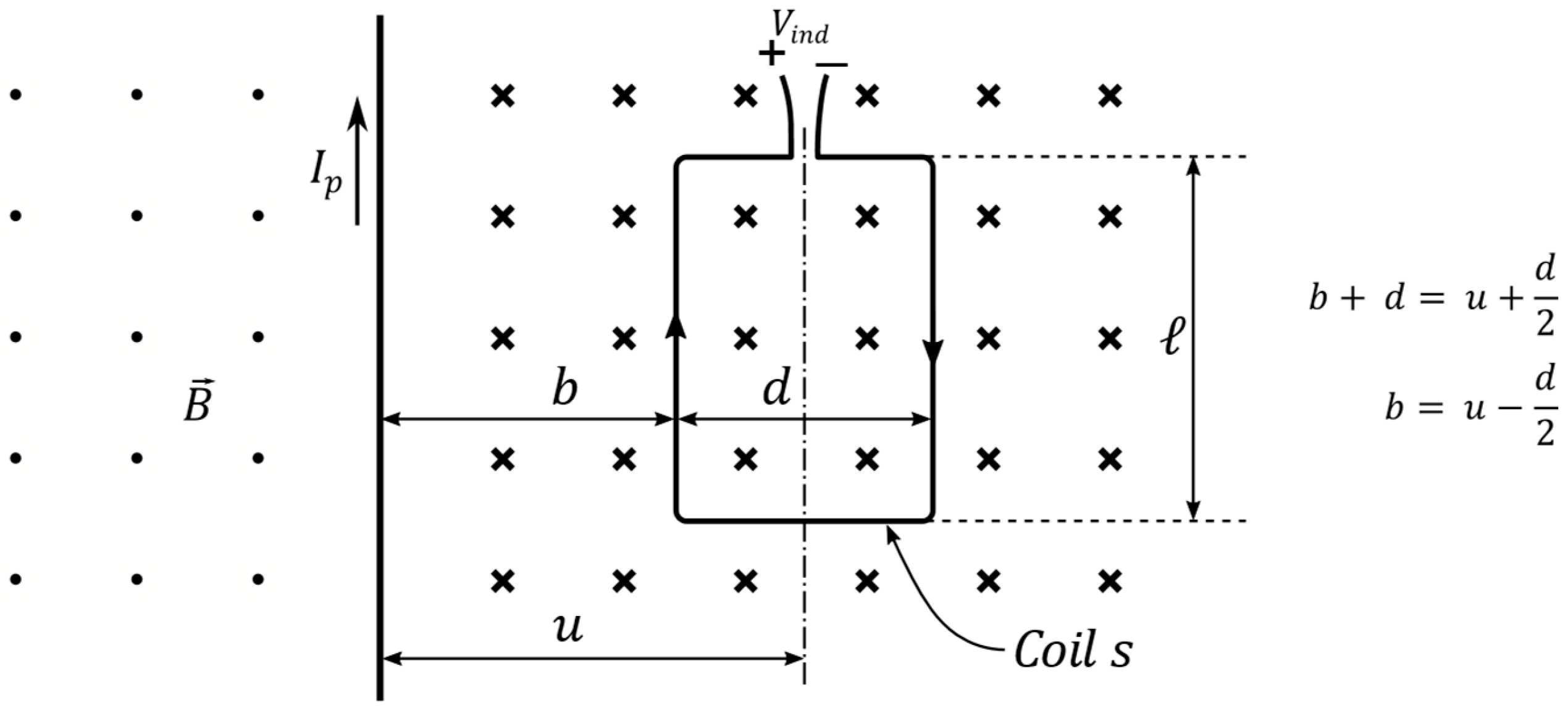
Lemma 1.

The voltage $V_{ind}$ induced on a rectangular coil $s$, constituted by a single turn of filamentary wire, due to an infinitely long, straight, parallel filamentary wire p, carrying a sinusoidal current $I_p$ of constant amplitude and frequency $f_0=2\pi {\omega }_0$, when $s$ is stationary relative to $p$ and located at distance $h$ from the plane that contains $p$, is given by

$${\dot{V}}_{ind}=-j \mu f_0 {\dot{I}}_p \mathcal{l}{\displaystyle \frac{1}{2}}\mathrm{l}\mathrm{n}{\displaystyle \frac{{\left(u-\frac{d}{2}\right)}^2+h^2}{{\left(u+\frac{d}{2}\right)}^2+h^2}},$$

(4)

where

-

${\dot{V}}_{ind}$ is the phasor representation of the voltage $V_{ind}$;

-

$\mu$ is the magnetic permeability of the medium where the conductors are immersed;

-

${\dot{I}}_p$ is the phasor representing current $I_p$;

-

$\mathcal{l}$ is the length of the side of the rectangular coil $s$ that is parallel to the wire p;

-

$d$ is the length of the side of the rectangular coil $s$ that is perpendicular to $p$;

-

$u$ is the oriented displacement of $p$ relative to the center plane of $s$, which is perpendicular to the plane of $s$ and parallel to $p$.

-

$j∊\mathbb{C}$, $j^2=-1$

With $p$ being a filamentary wire, it is assumed that, regarding its effect on other conductors, the current traversing wire $p$ can be considered concentrated on a single line support of $p$, analogous to what is happening to the filamentary wire $s$, which is assumed to only contain a single path where the electric field can be integrated. This assumption will approximate real problems where the distances between conductors are much greater than their diameters. Remarkably, when this assumption does not hold, (4) will visibly fail when $p$ excessively approaches one of the conductors that are the parallel to $p$ sides of the rectangular coil $s$. That is, expression (4) clearly diverges to infinity when, simultaneously, $h \to 0$ and either $u \to d/2$ or $u \to -d/2$, while it is known from experimentation that, in this case, the induced voltage $V_{ind}$ approaches the voltage across the segment of $p$ with length $\mathcal{l}$ that is closest to $s$.

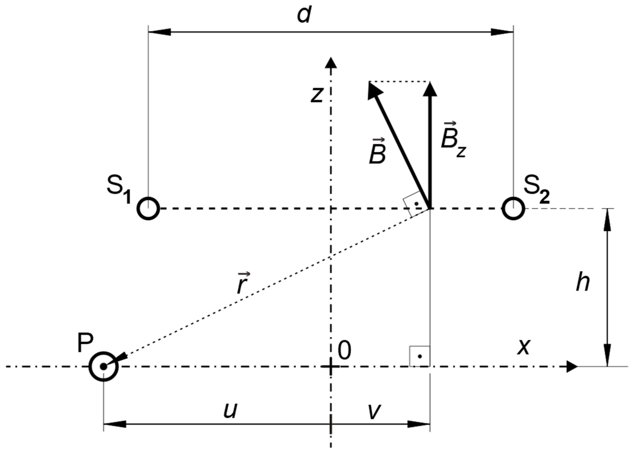
Proof of Lemma 1.

For the visualization of the geometry involved in the problem, let us start by considering the cross-section of this configuration, where $p$ is inducing a voltage in coil $s$, as shown in Figure 2, where the above linear dimensions are indicated, except $\mathcal{l}$, which is taken as perpendicular to the cross-section.

Figure 2. Reference cross-section for Lemma 1.

Let $S_1$, $S_2$, and P be, respectively, the points where coil $s$ and wire $p$ intercept this cross-section. Let $\overrightarrow{B}$ be the magnetic field generated by ${\dot{I}}_p$ flowing on p, and ${\dot{B}}_z$ its complex scalar component on axis $z$, which is perpendicular to the plane containing $s$.

In order to compute the induced voltage on $s$, Maxwell’s equation of Faraday’s Law can be used to express the induced voltage as the time derivative of the magnetic flux traversing coil $s$:

$$V_{ind}=\underset{s}{\oint }\overrightarrow{E}.\overrightarrow{ds}=-{\displaystyle \frac{d}{dt}}\underset{A}{\int }\overrightarrow{B}.\overrightarrow{dA},$$

(5)

where $\overrightarrow{E}$ is the electric field induced on the path corresponding to the thin wire coil $s$, $\overrightarrow{ds}$ is the differential element of the path of s, $\overrightarrow{A}$ is the oriented rectangular surface enclosed by $s$, and $\overrightarrow{dA}$ is its oriented differential area element.

Expression (5) can be rewritten using phasors, and considering the existing planar symmetry of $\overrightarrow{B}$ due to the infinite length of $p$, leading to

$${\dot{V}}_{ind}=-{\displaystyle \frac{d}{dt}}\underset{-{\displaystyle \frac{d}{2}}}{\overset{{\displaystyle \frac{d}{2}}}{\int }}{\dot{B}}_z \mathcal{l} dv$$

(6)

Considering no relative movement of the coil $s$ (quasi-stationary approximation) with respect to the wire $p$, the magnetic flux on $s$ is only a function of the time, so

$${\dot{V}}_{ind}=-\underset{-{\displaystyle \frac{d}{2}}}{\overset{{\displaystyle \frac{d}{2}}}{\int }}{\displaystyle \frac{d}{dt}}{\dot{B}}_z \mathcal{l} dv=-j\omega \mathcal{l}\underset{-{\displaystyle \frac{d}{2}}}{\overset{{\displaystyle \frac{d}{2}}}{\int }}{\dot{B}}_z dv$$

(7)

For an infinitely long thin wire $p$, the magnetic field $\overrightarrow{B}$ on any point of space is perpendicular to $p$, and thus contained in the plane parallel to the cross-section, being tangential to a circle of radius $r$ centered at P passing on that point of space, with complex magnitude given by

$$\dot{B}={\displaystyle \frac{\mu {\dot{I}}_p }{2\pi r}}$$

(8)

It can be observed that

$${\dot{B}}_z=\dot{B}\cos \theta = {\displaystyle \frac{\mu {\dot{I}}_p }{2\pi r}} {\displaystyle \frac{\left(v-u\right)}{r}}={\displaystyle \frac{\mu {\dot{I}}_p }{2\pi }} {\displaystyle \frac{\left(v-u\right) }{h^2+{\left(v-u\right)}^2}}$$

(9)

Combining (7) and (9), and considering that $\omega =2\pi f_0$,

$${\dot{V}}_{ind}=-j \mu f_0 {\dot{I}}_p \mathcal{l}\underset{-{\displaystyle \frac{d}{2}}}{\overset{{\displaystyle \frac{d}{2}}}{\int }}{\displaystyle \frac{\left(v-u\right) }{h^2+{\left(v-u\right)}^2}}dv$$

(10)

The integral in (10) can be calculated by substitution, using $r$ again:

$$r=\sqrt{h^2+{\left(v-u\right)}^2}$$

(11)

$$\Rightarrow r{\displaystyle \frac{dr}{dv}}=\left(v-u\right)$$

(12)

$${\dot{V}}_{ind}=-j \mu f_0 {\dot{I}}_p \mathcal{l}\underset{\sqrt{{\left(u+{\displaystyle \frac{d}{2}}\right)}^2+h^2}}{\overset{\sqrt{{\left(u-{\displaystyle \frac{d}{2}}\right)}^2+h^2}}{\int }}{\displaystyle \frac{1 }{r}}dr ,$$

(13)

which can be integrated as

$${\dot{V}}_{ind}=-j \mu f_0 {\dot{I}}_p \mathcal{l}{\displaystyle \frac{1}{2}} \left(\ln \left({\left(u-{\displaystyle \frac{d}{2}}\right)}^2+h^2\right)-\ln \left({\left(u+{\displaystyle \frac{d}{2}}\right)}^2+h^2\right)\right),$$

(14)

which is an equivalent expression to (4). □

In stationary IWPT (and, by approximation, in quasi-stationary DIWPT), the problem of calculating the induced voltage is equivalent to the calculation of the mutual inductance between the rectangular coil and the infinitely long parallel wire. A trivial case of Lemma 1, where $h=0$, often referred in textbooks [33], is illustrated in Figure 3.

Figure 3. Trivial case of Lemma 1 with $h=0$.

In this case, the magnetic flux traversing coil $s$ (into the paper), ${\Phi }_s$, is given by [33]

$${\Phi }_s=\mu I_p \mathcal{l}{\displaystyle \frac{1}{2\pi }} \ln {\displaystyle \frac{b+d}{b}} ,$$

(15)

leading to the calculation of ${\dot{V}}_{ind}$:

$${\dot{V}}_{ind}=j \mu {\omega }_0 {\dot{I}}_p \mathcal{l}{\displaystyle \frac{1}{2\pi }} \ln {\displaystyle \frac{b+d}{b}}=-j \mu f_0 {\dot{I}}_p \mathcal{l}\ln {\displaystyle \frac{u-\frac{d}{2}}{u+\frac{d}{2}}} ,$$

(16)

which is consistent with (2) when $h=0.$

The obtained expression for ${\dot{V}}_{ind}$ in Lemma 1 (2) is implicitly associated with the reference polarity of the terminals of coil $s$, where the right-hand rule is used for the closed curve integration of the induced electric field on $s$. Considering the geometry in Figure 2, the real and imaginary parts of current ${\dot{I}}_p$ are positive when coming out of paper, and ${\dot{V}}_{ind}$ expresses the differential electric potential $V_1-V_2$, between the left ($S_1$) and right ($S_2$) terminals of $s$, seen from the front of the paper, when $s$ is in open-circuit condition. If the polarity convention is reverse direction, that is, measuring $V_1-V_2$, $V_{ind}$ would alternatively be given by the phasor ${\dot{V}}_{-ind}$:

$${\dot{V}}_{-ind}=j{\displaystyle \frac{\mu f_0 {\dot{I}}_p \mathcal{l}}{2}}\ln {\displaystyle \frac{{\left(u-\frac{d}{2}\right)}^2+h^2}{{\left(u+\frac{d}{2}\right)}^2+h^2}}=-j{\displaystyle \frac{\mu f_0 {\dot{I}}_p \mathcal{l}}{2}}\ln {\displaystyle \frac{{\left(u+\frac{d}{2}\right)}^2+h^2}{{\left(u-\frac{d}{2}\right)}^2+h^2}}$$

(17)

In (3), it is still possible to factorize ${\dot{V}}_{ind}$ as

$${\dot{V}}_{ind}=-j \mu f_0 {\dot{I}}_p \mathcal{l} g\left(u,h,d\right) ,$$

(18)

where $g$ is function of the geometry of the cross-section of the physical problem:

$$g\left(u,h,d\right)={\displaystyle \frac{1}{2}}\ln {\displaystyle \frac{{\left(u-\frac{d}{2}\right)}^2+h^2}{{\left(u+\frac{d}{2}\right)}^2+h^2}}$$

(19)

The expression $\mu f_0{\dot{I}}_p\mathcal{l}$ depends on physical parameters that are not related to the geometry of its cross-section and assumed to be constant. So, for simplicity, it makes sense to interpret $g\left(u,h,d\right)$ as a normalized induced voltage, defined by a real-valued phasor:

$${\dot{G}}_{ind}={\displaystyle \frac{{\dot{V}}_{ind}}{-j \mu f_0 {\dot{I}}_p \mathcal{l}}}=g\left(u,h,d\right) ,$$

(20)

Having $h>0$ and $d>0$ as constant parameters, $g$ can be momentarily redefined as a function of $u$ only, and verified to be anti-symmetric, i.e., for all $u\in \mathbb{R}$,

$$g\left(-u\right)=-g\left(u\right),$$

(21)

It can be noticed that $g$ can be expressed as a multiplication of two functions, $g_1$ and $g_2$, that are each a composition of functions, namely, $\left[\ln x\right]$, $\left[x^2\right]$, $\left[x^2+h^2\right]$, $\left[x-{\displaystyle \frac{d}{2}}\right]$, and $\left[x+{\displaystyle \frac{d}{2}}\right]$, which are continuous and continuously n-differentiable in their domains, for all orders n $\ge 1$:

$$g\left(u\right)=g_1\left(u\right)\ast g_2\left(u\right),$$

(22)

where

$$g_1\left(u\right)=\left[\ln x\right]\circ \left[x^2\right]\circ \left[x^2+h^2\right]\circ \left[x-{\displaystyle \frac{d}{2}}\right]\left(u\right) ,$$

(23)

$$g_2\left(u\right)=\left[\ln x\right]\circ \left[x^2\right]\circ \left[{\displaystyle \frac{1}{x}}\right] \circ \left[x^2+h^2\right]\circ \left[x+{\displaystyle \frac{d}{2}}\right]\left(u\right)$$

(24)

Also, the image of each function in the chain composing both $g_1$ and $g_2$ is contained in the domain of the following function in the chain that takes the output of the former as its input. Then, $g\left(u\right)$ is also n-differentiable in $\mathbb{R}$, and from (28) it follows that

$${\left.{\displaystyle \frac{{\partial }^{n}g}{\partial u^n}}\right|}_{-u}=-{\left(-1\right)}^n{\left.{\displaystyle \frac{{\partial }^{n}g}{\partial u^n}}\right|}_u$$

(25)

and thus

$${\left.{\displaystyle \frac{{\partial }^{2n-1}g}{\partial u^{2n-1}}}\right|}_u={\left.-{\displaystyle \frac{{\partial }^{2n-1}g}{\partial u^{2n-1}}}\right|}_u, n\ge 1$$

(26)

$${\left.{\displaystyle \frac{{\partial }^{2n}g}{\partial u^{2n}}}\right|}_{u=0}={\left.-{\displaystyle \frac{{\partial }^{2n}g}{\partial u^{2n}}}\right|}_{u=0} \Rightarrow {\left.{\displaystyle \frac{{\partial }^{2n}g}{\partial u^{2n}}}\right|}_{u=0}=0, n\ge 1$$

(27)

By developing $\partial g/\partial u$ and ${\partial }^{3}g/\partial u^3$, it can be found that

$${\left.{\displaystyle \frac{\partial g}{\partial u}}\right|}_{u=0}=-{\displaystyle \frac{4d}{d^2+4h^2}} ,$$

(28)

$${\left.{\displaystyle \frac{{\partial }^{3}g}{\partial u^3}}\right|}_{u=0}=-{\displaystyle \frac{32d(d^2-12h^2)}{{(d^2+4h^2)}^3}}$$

(29)

Considering Equations (25)–(29), the Taylor expansion of $g$ to the fourth order, in the vicinity of the center of coil s, which is at $u=0$, with $h$ and $d$ fixed, it is possible to approximate $g\left(u,h,d\right)$ by

$$g\left(u,h,d\right)\cong -{\displaystyle \frac{4d}{d^2+4h^2}}u-{\displaystyle \frac{16d(d^2-12h^2)}{3{(d^2+4h^2)}^3}}{u}^3$$

(30)

So, given that the second and fourth derivatives of $g$ are already zero at $u=0$, the dependence of the induced voltage $g$ on the lateral displacement $u$, in the vicinity of the center of coil $s$, will be maximally linearized when the third derivative of $g$, given by (28), is also zero at $u=0$. This happens when

$$d^2-12h^2=0$$

(31)

$$\Rightarrow {\displaystyle \frac{h}{d}}={\displaystyle \frac{1}{2\sqrt{3}}}={\gamma }_h$$

(32)

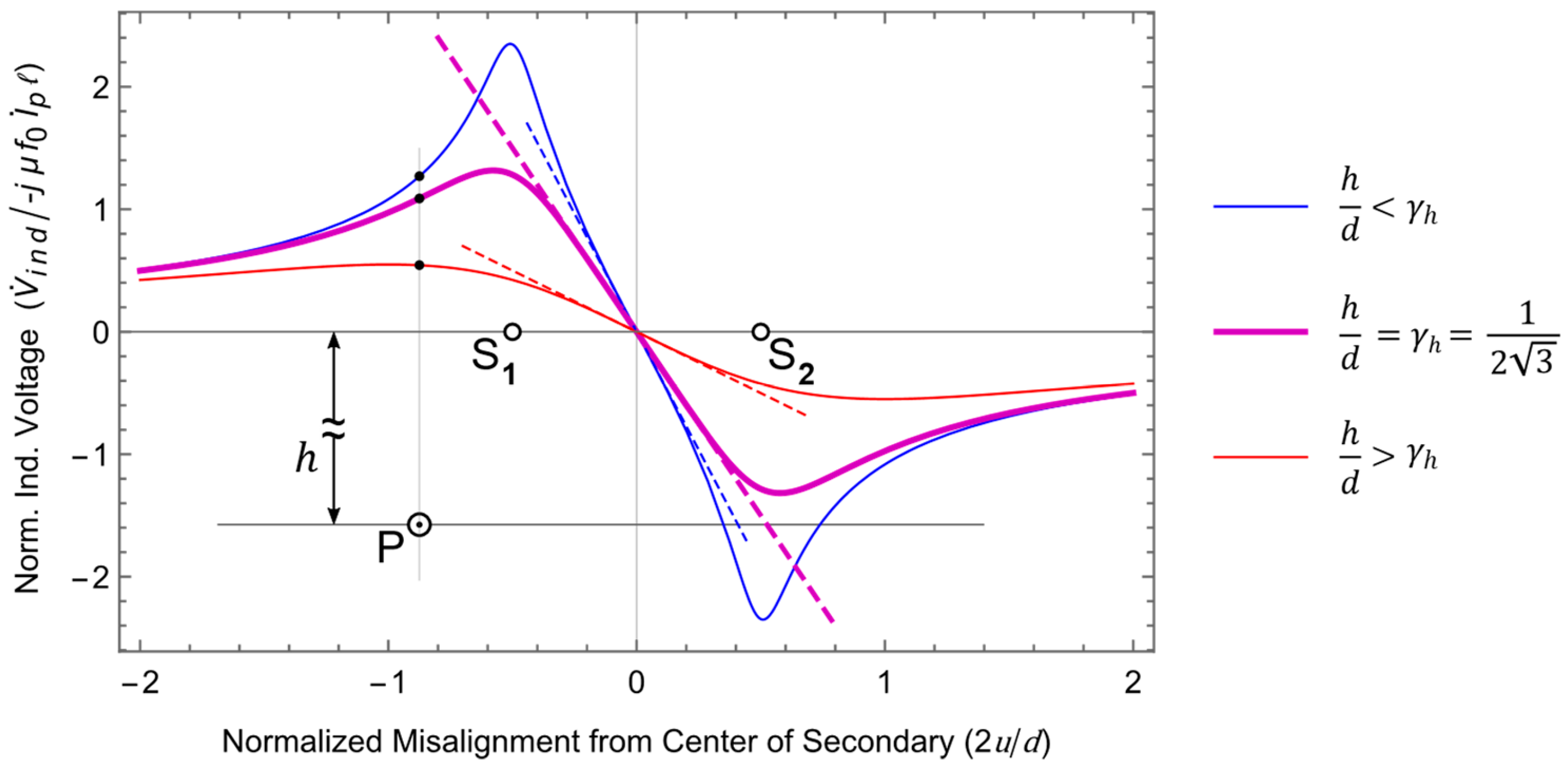
In Figure 4, the normalized induced voltage $g\left(u,h,d\right)$ is plotted as a function of the normalized displacement $2u$/d for different ratios $h/d$, emphasizing the case where the best linearity response is found, when $h/d={\gamma }_h$.

Figure 4. Profile of voltage induced on coil $s$ by a wire $p$ at distance $h$.

It can also be observed in Figure 4 that the curves corresponding to the normalized induced voltage, and thus to the induced voltage itself, exhibit maximum and minimum values at distances to the center of the coils that should be equal, except for the signal, which is due to the symmetric nature of the configuration. These points of maximum and minimum, which appear to depart from the center of $s$ as the ratio $h/d$ is increased, are the matter of the following Lemma 2.

Lemma 2.

Given a rectangular coil $s$ and a parallel wire $p,$ under the same assumptions and parameters described for Lemma 1, the maximum and the minimum induced voltages on $s$ are obtained when the oriented displacement of $p$ relative to center plane of s, which is perpendicular to the plane containing s and parallel to $p$, are, respectively, given by

$$u_{max}=-{\displaystyle \frac{1}{2}}\sqrt{d^2+4h^2}$$

(33)

$$u_{min}=+{\displaystyle \frac{1}{2}}\sqrt{d^2+4h^2}$$

(34)

Proof of Lemma 2.

For the visualization of the geometry involved in the problem, Figure 2, used in Lemma 1, is equally applicable. Referring to expression (18), it can be realized that the maximization or minimization of ${\dot{V}}_{ind}$ is, respectively, obtained by the maximization or minimization of the function $g$ with respect to the oriented distance $u$. This is carried out by requiring the following:

(i).

For the maximum:

$${\displaystyle \frac{\partial g}{\partial u}}=0 \wedge {\displaystyle \frac{{\partial }^{2}g}{\partial u^2}}<0$$

(35)

(ii).

For the minimum:

$${\displaystyle \frac{\partial g}{\partial u}}=0 \wedge {\displaystyle \frac{{\partial }^{2}g}{\partial u^2}}>0$$

(36)

Developing the expressions in (34) and (35),

$${\displaystyle \frac{\partial g}{\partial u}}\left(u,h,d\right)=-{\displaystyle \frac{4d(d^2+4h^2-4u^2)}{(4h^2+{(d-2u)}^2)(4h^2+{(d+2u)}^2)}}$$

(37)

$${\displaystyle \frac{{\partial }^{2}g}{\partial u^2}}\left(u,h,d\right)={\displaystyle \frac{32du\left(16h^2\right(d^2+4h^2+4u^2)-AB)}{A^2{B}^2}}$$

(38)

where

$$A=4h^2+{(d-2u)}^2>0$$

(39)

$$B=4h^2+{(d+2u)}^2>0$$

(40)

Requiring $\partial g/\partial u=0$ implies solving the following equation:

$$d^2+4h^2-4u^2=0 ,$$

(41)

which gives the following two solutions:

$$q_1=-{\displaystyle \frac{1}{2}}\sqrt{d^2+4h^2} ,$$

(42)

$$q_2={\displaystyle \frac{1}{2}}\sqrt{d^2+4h^2} ,$$

(43)

Evaluating ${\partial }^{2}g/\partial u^2$ at $q_1$ and $q_2$ results in

$${\displaystyle \frac{{\partial }^{2}g}{\partial u^2}}\left(u_1,h,d\right)=-{\displaystyle \frac{256 d h^2{\left(d^2+4h^2\right)}^{3/2}}{A^2{B}^2}}<0$$

(44)

$$\Rightarrow {u_{max}=q}_1=-{\displaystyle \frac{1}{2}}\sqrt{d^2+4h^2}$$

(45)

and

$${\displaystyle \frac{{\partial }^{2}g}{\partial u^2}}\left(u_2,h,d\right)={\displaystyle \frac{256 d h^2{\left(d^2+4h^2\right)}^{3/2}}{A^2{B}^2}}>0$$

(46)

$$\Rightarrow {u_{min}=q}_2={\displaystyle \frac{1}{2}}\sqrt{d^2+4h^2}$$

(47)

Expressions for the displacements of $p$ that maximize and minimize the induced voltage on coil $s$, given by (45) and (47), respectively, coincide with (33) and (34). □

A direct application of either Lemma 1 or Lemma 2 to the design of a DIWPT configuration is not likely, because a primary coil is not usually formed of a single conductor. However, based on these lemmas, it is possible to easily derive the expression of induced voltage on a rectangular coil over an oblong primary coil, and some useful relations involving optimal dimensional parameters, which is of interest for designing DIWPT configurations using oblong coils.

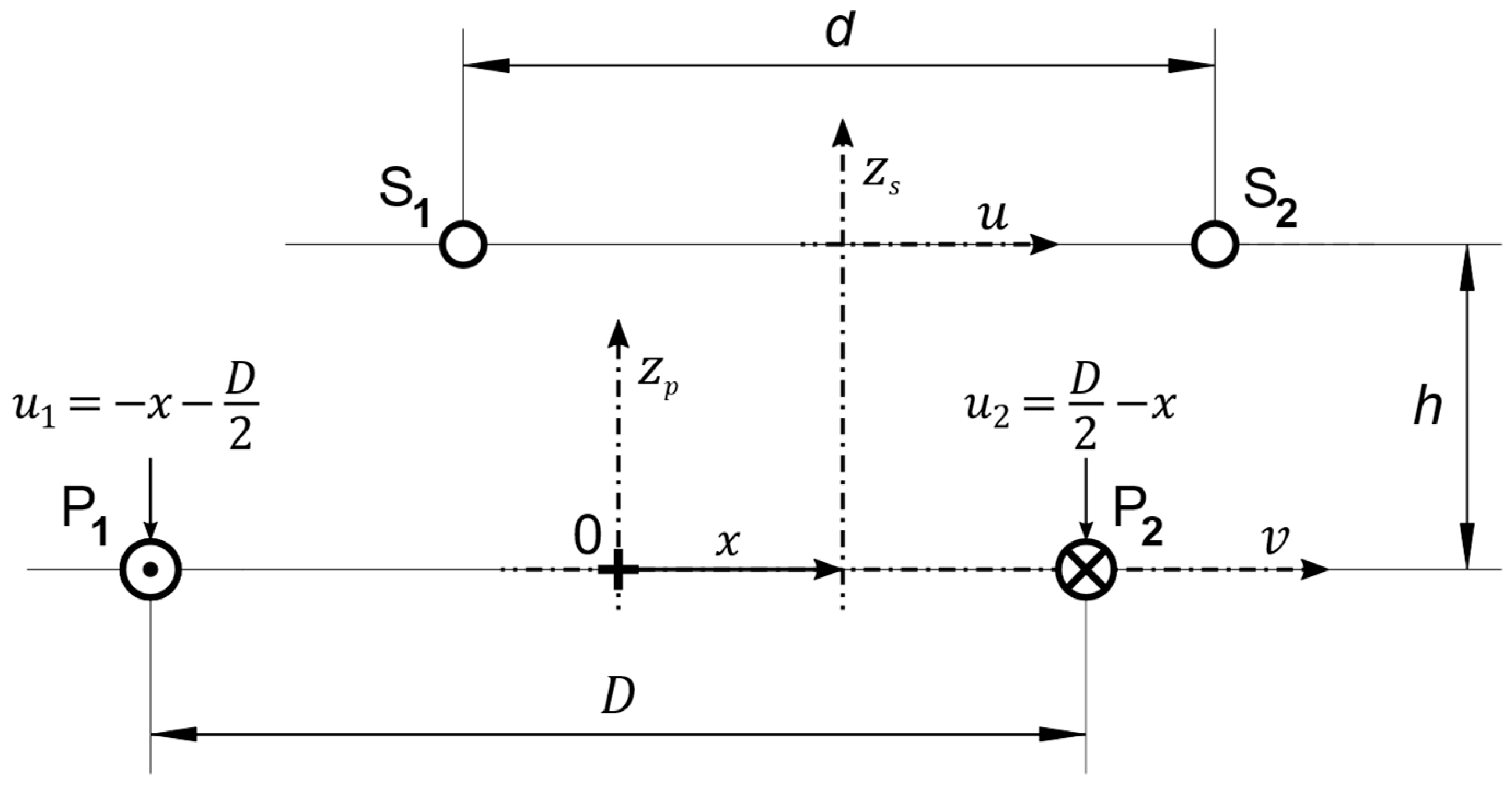
3.1. Expression of the Voltage Induced by an Oblong Coil on a Parallel, Rectangular Secondary Coil at a Given Distance from the Plane Containing the Oblong Coil

Theorem 1.

The voltage $V_{ind}$ induced by a stationary, infinitely long coil p, constituted of a single turn of a filamentary wire carrying a sinusoidal current $I_p$ of constant amplitude and frequency $f_0=2\pi {\omega }_0$, on a parallel rectangular coil $s$, stationary relative to $p$ and also constituted of a single turn of a filamentary wire, which is located on a plane that is parallel to the plane that contains $p$, at a distance $h$ to that plane, is given by

$${\dot{V}}_{ind}=-j \mu f_0 {\dot{I}}_p \mathcal{l}\xi \left(x,h,d,D\right) ,$$

(48)

with the real function $\xi$ given by

$$\xi \left(x,h,d,D\right)={\displaystyle \frac{1}{2}}\ln {\displaystyle \frac{\left({\left(x+\frac{D+d}{2}\right)}^2+h^2\right)\left({\left(x-\frac{D+d}{2}\right)}^2+h^2\right)}{\left({\left(x+\frac{D-d}{2}\right)}^2+h^2\right)\left({\left(x-\frac{D-d}{2}\right)}^2+h^2\right)}} ,$$

(49)

where

-

${\dot{V}}_{ind}$ is the phasor representation of the voltage $V_{ind}$;

-

$\mu$ is the magnetic permeability of the medium where the conductors are immersed;

-

${\dot{I}}_p$ is the phasor representing current $I_p$;

-

$\mathcal{l}$ is the length of the side of the rectangular coil $s$ that is parallel to the wire p;

-

$D$ is the width of the infinitely long coil $p$, i.e., the distance between its two conductors;

-

$d$ is the length of the side of the rectangular coil $s$ that is perpendicular to $p$;

-

$x$ is the oriented displacement of the projection of the longitudinal axis of s on the plane of p to the longitudinal axis of p (if p and s are contained in horizontal planes, $x$ is the lateral misalignment between these coils).

-

$j∊\mathbb{C}$, $j^2=-1$

Again, the term filamentary wire is used here in the same sense and with the same assumptions as used for Lemmas 1 and 2.

Proof of Theorem 1.

For the visualization of the geometry involved in the problem, let us start by considering a cross-section of this configuration, where coil $p$ is inducing a voltage in coil $s$, as shown in Figure 5, with equivalently defined parameters as in Figure 2, where $S_1$.

Figure 5. Cross-section of the inductive configuration formed by coils $p$ and $s$.

Applying the superposition principle to the magnetic fields generated by the currents traversing the two wires of coil p, it can be derived that the total induced voltage will be the sum of the two voltages separately induced by currents $I_p$ flowing out of the paper at $P_1$ and inwards at $P_2$, which is equivalent to a current ${-I}_p$ flowing out of the paper. Then, from Lemma 1, it is possible to use (18) twice, adding up the voltages induced on $s$ by the conductor of $p$ at $P_1$, ${\dot{V}}_1$, and by the conductor of $p$ at $P_2$,${\dot{V}}_1$:

$${\dot{V}}_1=-j \mu f_0 {\dot{I}}_p \mathcal{l} g(u_1,h,d)$$

(50)

$${\dot{V}}_2=-j \mu f_0\left(-{\dot{I}}_p\right) \mathcal{l} g(u_2,h,d)$$

(51)

$${\dot{V}}_{ind}={\dot{V}}_1+{\dot{V}}_2=-j \mu f_0 {\dot{I}}_p \mathcal{l}\left(g\left(-x-{\displaystyle \frac{D}{2}},h,d\right)-g\left({\displaystyle \frac{D}{2}}-x,h,d\right)\right)$$

(52)

Applying (19) to expand the function g, (52) becomes

$${\dot{V}}_{ind}=-j \mu f_0{\dot{I}}_p\mathcal{l}{\displaystyle \frac{1}{2}}\left(\ln {\displaystyle \frac{{\left(-x-\frac{D}{2}-\frac{d}{2}\right)}^2+h^2}{{\left(-x-\frac{D}{2}+\frac{d}{2}\right)}^2+h^2}}-\ln {\displaystyle \frac{{\left(\frac{D}{2}-x-\frac{d}{2}\right)}^2+h^2}{{\left(\frac{D}{2}-x+\frac{d}{2}\right)}^2+h^2}}\right)$$

(53)

Reorganizing the terms of (53) results in

$${\dot{V}}_{ind}=-j \mu f_0{\dot{I}}_p\mathcal{l}{\displaystyle \frac{1}{2}}\ln {\displaystyle \frac{\left({\left(x+\frac{D+d}{2}\right)}^2+h^2\right)\left({\left(x-\frac{D+d}{2}\right)}^2+h^2\right)}{\left({\left(x+\frac{D-d}{2}\right)}^2+h^2\right)\left({\left(x-\frac{D-d}{2}\right)}^2+h^2\right)}} ,$$

(54)

which can be decomposed in expressions (48) and (50). □

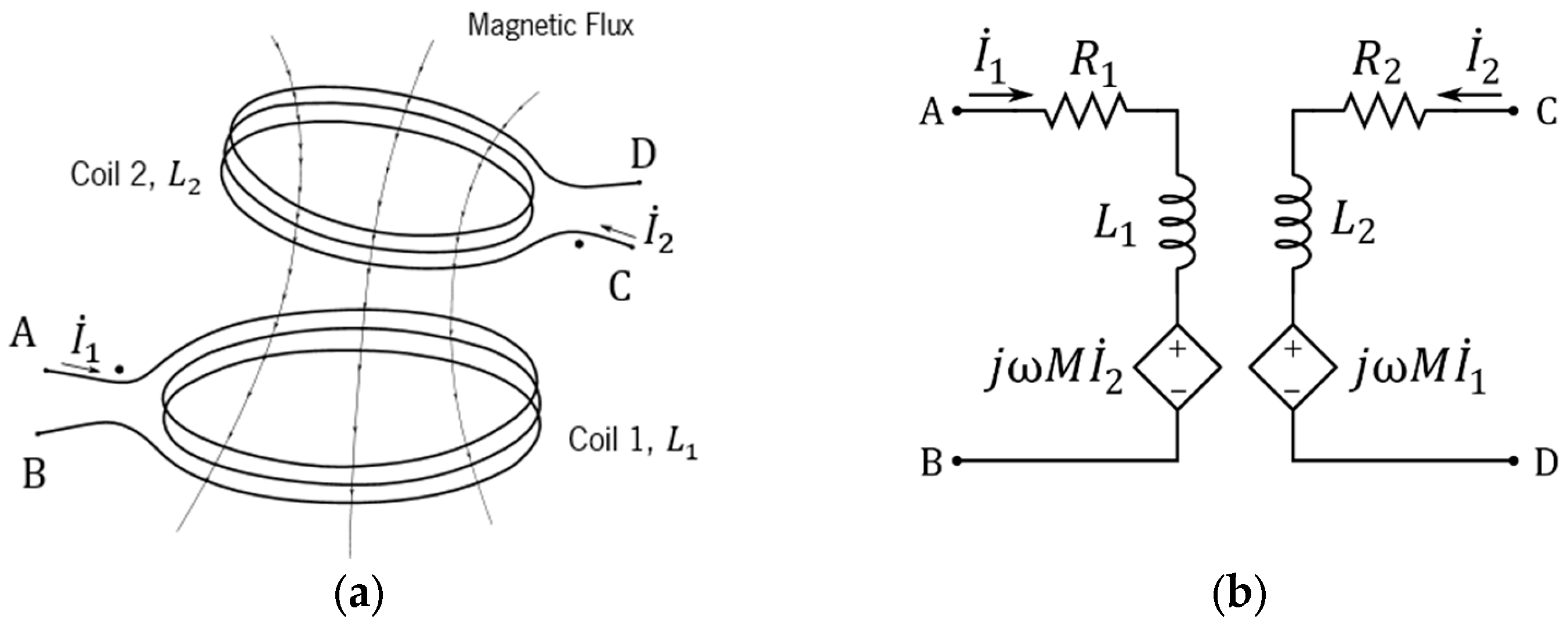
The expression for ${\dot{V}}_{ind}$ (48) can be compared to the model in Figure 1b, permitting the mutual inductance $M$ between $s$ and the long coil p to be equivalently expressed as follows:

$$M={\displaystyle \frac{\mu }{2\pi }} \mathcal{l} \xi \left(x,h,d,D\right),$$

(55)

Illustrating a possible application of Theorem 1, Figure 6 shows the scalar field of the normalized induced voltage, ξ, computed using (49), on the cross-section of an inductive configuration with an infinitely long primary filamentary coil $p$ and a parallel rectangular filamentary coil $s$, each consisting of a single turn.

Figure 6. Normalized voltage induced on a single-turn secondary coil $s$ by a single-turn primary coil $p$ as a function of the relative position of the center of $s$ to $p$, under the hypotheses of Theorem 1.

The conductors of the primary coil $p$, indicated in Figure 6 by two red dots, are placed centered at $h=0$. The conductors of the secondary coil s are indicated by two dark blue dots, $S_1$ and $S_2$, and probe the induced voltage when translated over the cross-section, a typical situation of interest in the design of DIWPT configurations. Specifically, for this example, the ratio $D/d$ was set to $2/\sqrt{3}$. The red curve exemplifies a possible path for the displacement of $s$, with the red cross denoting the center of the secondary coil $s$. The color of the plot shows how the value of the normalized induced voltage, $\xi$, changes when the center of the secondary coil is displaced on the cross-section plane. The blue regions indicate the positions of the cross-section, where $\xi >0$, i.e., ${\dot{V}}_{ind}$ is given by $j\alpha {\dot{I}}_p$, where $\alpha >0$, and the phase of $V_{ind}$ is $\pi /2$ ahead of the phase of $I_p$. Similarly, in the pink regions, the phase of $V_{ind}$ is a $\pi /2$ delayed form of the phase of $I_p$. The black dashed curves are the loci of the zero induced voltage, defined by the following equation:

$$\xi \left(x,h,d,D\right)=0 ,$$

(56)

where $d$ and $D$ are the fixed widths of, respectively, the secondary and primary coils, and $(x,h)$ is the coordinate pair of a point of the cross-section belonging to the dashed curve where $V_{ind}=0.$

Developing (56) results in an equation of $x$ and $h$:

$$\begin{gathered} \left({\left(x-{\displaystyle \frac{D+d}{2}}\right)}^2+h^2\right)\left({\left(x+{\displaystyle \frac{D+d}{2}}\right)}^2+h^2\right) \\ \hspace{1em}\hspace{1em}\hspace{1em}=\left({\left(x+{\displaystyle \frac{D-d}{2}}\right)}^2+h^2\right)\left({\left(x-{\displaystyle \frac{D-d}{2}}\right)}^2+h^2\right) \end{gathered}$$

(57)

which simplifies to

$$d^2+D^2+4h^2-4x^2=0 ,$$

(58)

which is the equation of a rectangular hyperbola on the plane $(x,h)$, with vertices ${\mathtt{H}}_1$ and ${\mathtt{H}}_2$ at

$${\mathtt{H}}_1=\left(-{\displaystyle \frac{\sqrt{d^2+D^2}}{2}},0\right)$$

(59)

$${\mathtt{H}}_2=\left(+{\displaystyle \frac{\sqrt{d^2+D^2}}{2}},0\right)$$

(60)

Remarkably, the fact that the loci of $V_{ind}=0$ form a rectangular hyperbola (eccentricity $\sqrt{2}$) does not depend on the ratio $d/D$, only its scale factor will depend on the indistinct sum of the squares of the coil widths.

Since in most vehicular DIWPT applications, the secondary coil is installed at a fixed distance from the primary coil, another useful application for Theorem 1 is to predict the induced voltage on a rectangular secondary coil as a function of the lateral misalignment on the lane, as exemplified in the curves of Figure 7, plotted in different colors tones for different ratios of $D/d$, increasing from 0.25 (red curve) to 2.5 (blue curve), and $h/d=1/2\sqrt{3}$.

Figure 7. Normalized voltage induced on a single-turn secondary coil $s$ that is at a fixed distance from the single-turn primary coil $p$ as a function of the relative position of the center of $s$ to $p$.

One key consideration to obtain a good numerical approximation for this prediction, using Theorem 1, is to require that the middle cross-section under analysis is far enough from the extremities of the primary coil. However, this is not a problem: while no actual oblong primary coil $p$ has infinite length, in practice, it is verified that the magnetic flux distribution generated by current $I_p$ is fairly regular along all its length, except very close to the extremities of $p$, when this coil is much longer than wide, and also much longer than the secondary coil.

3.2. Width of an Oblong Primary Coil for Maximum Induced Voltage on a Given Secondary Rectangular Coil at a Given Distance from the Primary Coil, Under Center Alignment Conditions

Theorem 2.

The maximum value of the normalized voltage $\xi ={\dot{V}}_{ind}/\left(-j\mu f_0{\dot{I}}_p\mathcal{l}\right)$ induced by a stationary, infinitely long filamentary coil p, of width $D$, which is constituted of a single turn of wire carrying a sinusoidal current $I_p$ of constant amplitude and frequency $f_0=2\pi {\omega }_0$, on a parallel rectangular coil $s$, of fixed width $d$ and length $\mathcal{l}$, also constituted of a single turn of filamentary wire, located on a plane that is parallel to the plane that contains $p$, at a fixed distance $h$ to that plane, is obtained when the coils are symmetrically aligned, with central planes coinciding, and the width $D$ of coil $p$ is equal to $w_P$:

$$w_P=\sqrt{d^2+4h^2}$$

(61)

and can be calculated by

$${\xi }_{{max}_{h,d}}=\ln {\displaystyle \frac{w_P+d}{w_P-d}}$$

(62)

Additionally, when the coils remain center-aligned and the width $D$ of the primary coil $p$ is varied, the normalized induced voltage observed with $D=\lambda w_P$ is the same as that observed when $D=w_P/\lambda$, for any $\lambda >0.$

Proof of Theorem 2.

This proof follows by initially applying Lemma 2 to each of the conductors of $p$, and separately positioning $P_1$ and $P_2$ in order to maximize the induced voltage. The property of the total magnetic flux on $s$ is the sum of the fluxes generated by $I_p$ leaving at $P_1$, and current ${-I}_p$ leaving at $P_2$, due to linear superposition of the respective magnetic fields generated by these two conductors of coil $p$, and the independence of the fields generated by them. Starting from Equations (50) to (52), it follows that

$${\dot{V}}_{ind}={\dot{V}}_1+{\dot{V}}_2$$

(63)

$$\underset{x}{\max }{\displaystyle \frac{{\dot{V}}_{ind}\left(x,h,d,D\right)}{-j \mu f_0 {\dot{I}}_p \mathcal{l}}}=\underset{x}{\max }{\displaystyle \frac{{\dot{V}}_1\left(x,h,d,D\right)}{-j \mu f_0 {\dot{I}}_p \mathcal{l}}}+\underset{x}{\max }{\displaystyle \frac{{\dot{V}}_2\left(x,h,d,D\right)}{-j \mu f_0 \left({\dot{I}}_p\right) \mathcal{l}}}$$

(64)

By Lemma 2,

$$\underset{x}{\max }{\displaystyle \frac{{\dot{V}}_1\left(x,h,d,D\right)}{-j \mu f_0 {\dot{I}}_p \mathcal{l}}}={\displaystyle \frac{{\dot{V}}_1\left(q_1,h,d,D\right)}{-j \mu f_0{ \dot{I}}_p \mathcal{l}}},\hspace{1em} q_1=-{\displaystyle \frac{1}{2}}\sqrt{d^2+4h^2}$$

(65)

Due to the anti-symmetry of ${\dot{V}}_2$, expressed in (20) and (21), to search for the maximum in normalized ${\dot{V}}_2$ is equivalent to searching for the minimum in normalized ${\dot{V}}_1$, and then the second parcel in (63) becomes

$$\underset{x}{\max }{\displaystyle \frac{{\dot{V}}_2\left(x,h,d,D\right)}{-j \mu f_0\left(-{\dot{I}}_p\right)\mathcal{l}}}=-\underset{x}{\min }{\displaystyle \frac{{\dot{V}}_1\left(x,h,d,D\right)}{-j \mu f_0\left({\dot{I}}_p\right)\mathcal{l}}}$$

(66)

which, by using Lemma 2 again, is found as

$$-\underset{x}{\min }{\displaystyle \frac{{\dot{V}}_1\left(x,h,d,D\right)}{-j \mu f_0\left({\dot{I}}_p\right)\mathcal{l}}}=-{\displaystyle \frac{{\dot{V}}_1\left(q_2,h,d,D\right)}{-j \mu f_0\left({\dot{I}}_p\right)\mathcal{l}}} , q_2={\displaystyle \frac{1}{2}}\sqrt{d^2+4h^2}$$

(67)

Hence, the normalized induced voltage on $s$ is maximized when the projections of the conductors of $p$, $P_1$ and $P_2$, are symmetrically placed around the center plane of coil $s$, $x=0$, at the following coordinates:

$$P_1: x=q_1=-{\displaystyle \frac{1}{2}}\sqrt{d^2+4h^2}$$

(68)

$$P_2: x=q_2= {\displaystyle \frac{1}{2}}\sqrt{d^2+4h^2}$$

(69)

and the optimum width $D=w_P$ of coil $p$ will then be given by the difference $q_2-q_1$:

$$w_P=q_2-q_1=\sqrt{d^2+4h^2} ,$$

(70)

which is identical to (61), thus comprising the first item of proof.

For this optimum width $w_P$ under the central alignment condition, the normalized maximum induced voltage can be further calculated by replacing $D$ in (49) by $w_P$, as given in (70):

$${\xi }_{{max}_{h,d}}=\xi \left(0,h,d,w_P\right)={\displaystyle \frac{1}{2}}\ln {\displaystyle \frac{{\left({\left(\frac{\sqrt{d^2+4h^2}+d}{2}\right)}^2+h^2\right)}^2}{{\left({\left(\frac{\sqrt{d^2+4h^2}-d}{2}\right)}^2+h^2\right)}^2}} ,$$

(71)

which can be simplified to

$${\xi }_{max}=\ln {\displaystyle \frac{\sqrt{d^2+4h^2}+d}{\sqrt{d^2+4h^2}-d}} ,$$

(72)

due to (70), an equivalent expression to (62), and this is the second part of the proof.

Finally, it can be calculated that, under the alignment condition, $x=0$, when $D=\lambda w_P$, $\lambda >0,$ the expression of $\xi$, given by Theorem 1 (49), becomes

$$\xi \left(0,h,d,\lambda w_P\right)=\ln {\displaystyle \frac{{\left(\frac{\lambda w_P+d}{2}\right)}^2+h^2}{{\left(\frac{\lambda w_P-d}{2}\right)}^2+h^2}} ,$$

(73)

which, by using (70), can be developed to

$$\xi \left(0,h,d,\lambda w_P\right)=\ln {\displaystyle \frac{w_P\left(1+{\lambda }^2\right)+2\lambda d}{w_P\left(1+{\lambda }^2\right)-2\lambda d}}$$

(74)

Based on (74), $\xi$, at $x=0$ and $D=w_P/\lambda ,$ is equal to

$$\xi \left(0,h,d,w_P/\lambda \right)=\ln {\displaystyle \frac{w_P\left(1+\frac{1}{{\lambda }^2}\right)+\frac{2d}{\lambda }}{w_P\left(1+\frac{1}{{\lambda }^2}\right)-\frac{2d}{\lambda }}}=\xi \left(0,h,d,\lambda w_P\right)$$

(75)

Hence, it follows that under the center alignment condition, the normalized induced voltages on coil $s$ are the same (and so are the induced voltages) when the width of the primary coil is either $\lambda w_P$ or $w_P/\lambda$, with $\lambda >0$. □

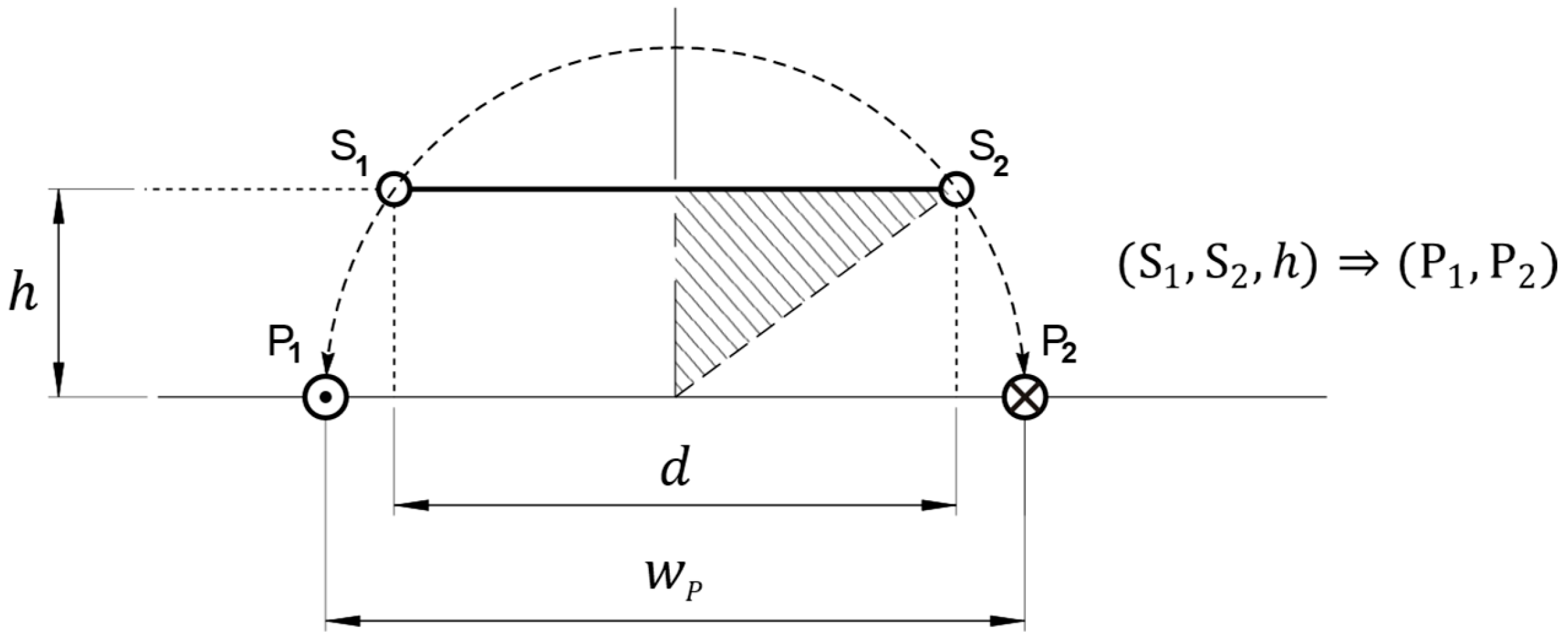
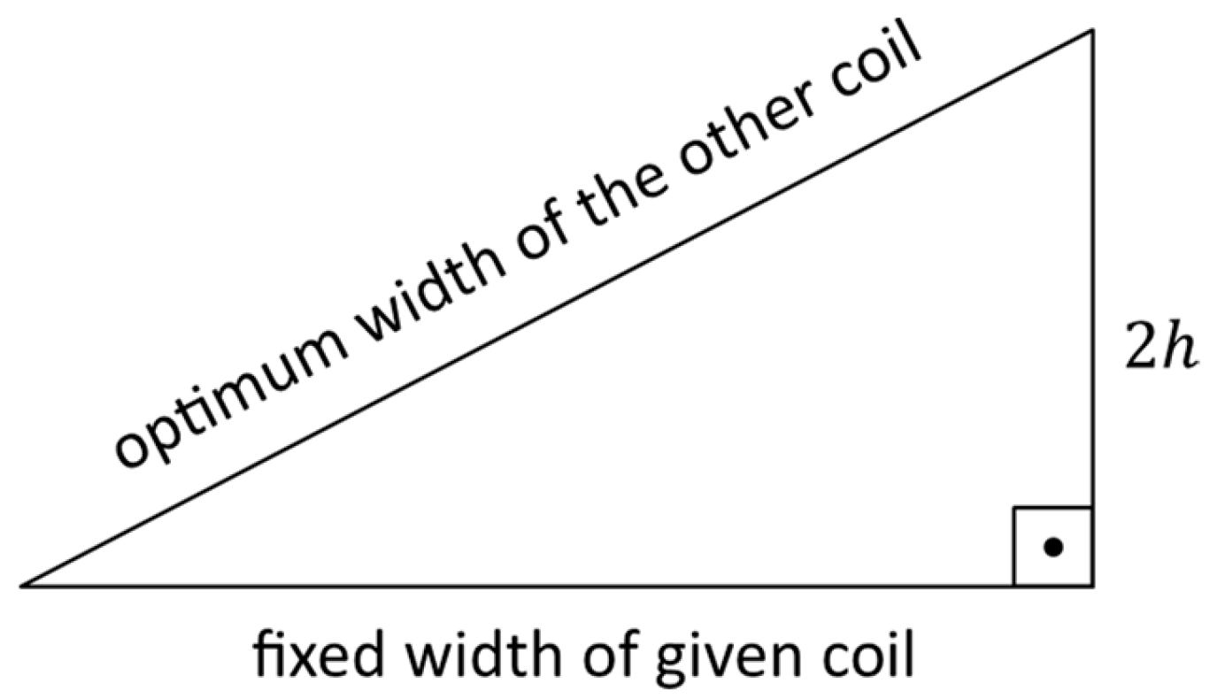
Geometric Interpretation for Theorem 2: Despite the tedious algebraic manipulation involved in Theorem 2, it has a simple immediate geometric interpretation: The infinitely long filamentary single-turn primary coil carrying a fixed sinusoidal current $I_p$ that will induce the maximum voltage on a parallel rectangular single-turn filamentary coil $s$ at distance $h$ from $p$ is the one in which the projection on a cross-section of this inductive configuration of the support lines of the conductors of $p$, $P_1$ and $P_2$, constitute the diameter $\overline{P_1{P}_2}$ of a circle also containing the projection of the support lines of the conductors of $s$, $S_1$ and $S_2$, as shown in Figure 8.

Figure 8. Geometrical interpretation of Theorem 2.

This relative positioning of $S_1$, $S_2$, $P_1$, and $P_2$ creates a right-angled rectangle where the vertical cathetus is $h$, the horizontal cathetus is $d/2$, and the hypotenuse, $D/2$, is calculated using Pythagoras’ theorem:

$${\left({\displaystyle \frac{D}{2}}\right)}^2={\left({\displaystyle \frac{d}{2}}\right)}^2+h^2={\left({\displaystyle \frac{w_P}{2}}\right)}^2$$

(76)

Hence, the geometrical construction in Figure 8 assures that $D=\sqrt{d^2+4h^2}$, which is the required width $w_P$ of $p$ for maximum induction in $s$.

3.3. Width of a Secondary Rectangular Coil at a Given Distance from a Given Oblong Primary Coil, for the Maximum Induced Voltage on the Secondary Coil Under Center Alignment Conditions

Theorem 3.

The maximum value for the normalized voltage $\xi ={\dot{V}}_{ind}/-j\mu f_0{\dot{I}}_p\mathcal{l}$ induced by a stationary, infinitely long filamentary coil p, of fixed width $D$, that is constituted of a single turn of wire carrying a sinusoidal current $I_p$ of constant amplitude and frequency $f_0=2\pi {\omega }_0$, on a parallel rectangular coil $s$, of width $d$ and length $\mathcal{l}$, also constituted of a single turn of filamentary wire, located on a plane that is parallel to the plane that contains $p$, at a fixed distance $h$ to that plane, is obtained when the coils are symmetrically aligned, with central planes coinciding, and the width $d$ of coil $s$ is equal to $w_S$:

$$w_S=\sqrt{D^2+4h^2}$$

(77)

 and can be calculated by

$${\xi }_{{max}_{h,D}}=\ln {\displaystyle \frac{w_S+D}{w_S-D}}$$

(78)

Additionally, when the coils remain center-aligned and the width $d$ of the primary coil $s$ is varied, the normalized induced voltage observed with $d=\lambda w_S$ is the same as that observed when $d=w_S/\lambda$, for any $\lambda >0.$

There is a duality relating Theorem 3 and Theorem 2; the expressions (77) and (78) are exactly the same as those in (61) and (62), except that $D$ and $w_S$ are used in place of $d$ and $w_P$. The physical situation in each case is different, though: In Theorem 2, the width of the secondary coil is fixed at $d$, and an optimal diameter of the primary coil, $D$, that maximizes the induced voltage on $s$ is to be found. Meanwhile, in Theorem 3, the search is reversed: the width $D$ of the primary coil itself is fixed, and an optimal width $d$ for the secondary coil that maximizes the induced on voltage $s$ is to be determined.

Proof of Theorem 3.

The reason for the above-mentioned duality, which is the proof for Theorem 3, is that, by inspection of the algebraic expression (49) of the function $\xi$, both the induced voltage from $p$ on $s$, ${\dot{V}}_{ind}$, as well as the associated normalized induced voltage, $\xi$, given by Theorem 1, are symmetric on $d$ and $D$:

$$\xi \left(x,h,d,D\right)=\xi \left(x,h,D,d\right),$$

(79)

and

$${\displaystyle \frac{{\partial }^n\xi }{\partial d^n}}={\displaystyle \frac{{\partial }^n\xi }{\partial D^n}} , \forall n\ge 1$$

(80)

Hence, the points of maxima in $\xi$, with respect to $d$, when $x=0$, are expressed in terms of fixed $h$ and $D$ by the same function as the points of maxima in $\xi$, when $x=0$, with respect to $D$, when expressed in terms of fixed $h$ and $d$, causing the width of the maximum induced voltage on s, at $x=0$, to also be found at an optimum value of $d$ and $w_S$, given as the function of $h$ and $D$:

$$w_S={\left.\sqrt{y^2+4h^2}\right|}_{y=D}=\sqrt{D^2+4h^2}$$

(81)

In the same manner, the value of the maxima will be given by the same function by which it was calculated in the case of the optimization in $D$, but evaluated at the pair $\left(h,D\right)$, rather than at the pair $\left(h,d\right)$:

$${\xi }_{max}={\left.\ln {\displaystyle \frac{\sqrt{y^2+4h^2}+y}{\sqrt{y^2+4h^2}-y}} \right|}_{y=D}=\ln {\displaystyle \frac{w_S+D}{w_S-D}}$$

(82)

To prove the last statement of Theorem 3, it can be realized that, for all $\lambda >0$,

$$\begin{gathered} \xi \left(0,h,\lambda w_S,D\right)=\xi \left(0,h,D,\lambda w_S\right) \\ ={\left.\xi \left(0,h,y,\lambda \sqrt{y^2+4h^2}\right)\right|}_{y=D}={\left.\xi \left(0,h,y,{\displaystyle \frac{\sqrt{y^2+4h^2}}{\lambda }}\right)\right|}_{y=D} \\ =\xi \left(0,h,D,{\displaystyle \frac{w_S}{\lambda }}\right)=\xi \left(0,h,{\displaystyle \frac{w_S}{\lambda }},D\right) , \end{gathered}$$

(83)

with the first and last equalities being due to the existing indistinguishability in $d$ and $D$, as given by (78), and the equality in the middle, due to Theorem 2. Hence,

$$\xi \left(0,h,\lambda w_S,D\right)=\xi \left(0,h,{\displaystyle \frac{w_S}{\lambda }},D\right) , \forall \lambda >0$$

(84)

which constitutes the last part of Theorem 3. □

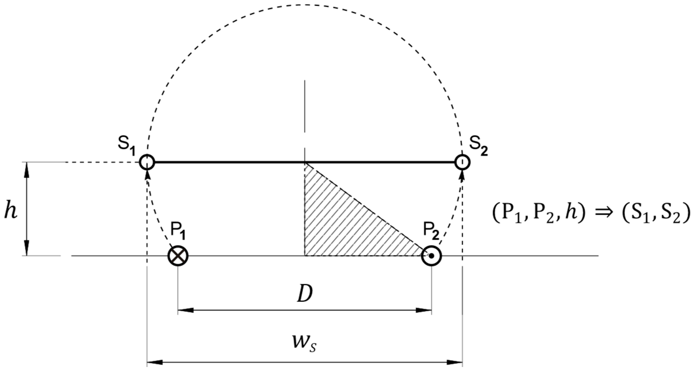
Geometric Interpretation for Theorem 3: Similarly to Theorem 2, the dimensions and location of the optimum filamentary secondary coil $s$ for a maximum induced voltage from a filamentary primary coil $p$, at a fixed distance $h$, also has a simple immediate geometric interpretation: if the projections of the support lines of the conductors of $p$, in a common cross-section with s, are $P_1$ and $P_2$, and the projections of the support lines of the conductors of $s$ parallel to $p$ are $S_1$ and $S_2$, then $S_1$ and $S_2$ constitute the diameter $\overline{S_1{S}_2}$ of a circle also containing $P_1$ and $P_2$, as shown in Figure 9.

Figure 9. Geometrical interpretation of Theorem 3.

Attention should be paid when comparing, using Theorem 2 and Theorem 3, which geometries can be visualized, respectively, in Figure 8 and Figure 9: the optimum width for the other coil, in order to attain maximum induced voltage on the secondary, is always larger than that of a first coil whose width has been fixed, no matter whether the first coil to have its dimensions fixed beforehand is the secondary or the primary coil, as synthetically represented in Figure 10.

Figure 10. Geometric interpretation of the optimum width of the other coil in an oblong coil configuration for maximum induced voltage.

3.4. Width of an Oblong Primary Coil for a Maximally Flat Induced Voltage on a Given Secondary Rectangular Coil at a Given Distance from the Primary Coil, Under Center Alignment Conditions

Theorem 4.

Let $p$ be a stationary, infinitely long filamentary coil p, of width $D$, that is constituted of a single turn of wire carrying a sinusoidal current $I_p$ of constant amplitude and frequency $f_0=2\pi {\omega }_0$; let $s$ be a rectangular coil parallel to $p$ of fixed width $d$ and length $\mathcal{l}$, also constituted of a single turn of filamentary wire and located on a plane that is parallel to the plane that contains $p$, at a fixed distance $h$ to that plane. Then, the profile of the normalized voltage $\xi ={\dot{V}}_{ind}/ j\mu f_0{\dot{I}}_p\mathcal{l}$, induced by $p$ on $s$, as a function of the lateral misalignment of $p$ and $s$, is maximally flat in the vicinity of the center alignment condition when the width $D$ of coil $p$ is either equal to $w_F$ or to $w_F^{\prime }$, as given by the following equations and conditions:

$$w_F=\sqrt{w_P^2+4w_{P}h} , h>0$$

(85)

$$w_F^{\prime }=\sqrt{w_P^2-4w_{P}h }, 0<{\displaystyle \frac{h}{d}}<{\gamma }_h$$

(86)

where  $w_P$ is the width of $p$ for the maximum induced voltage on s, as in Theorem 2:

$$w_P=\sqrt{d^2+4h^2},$$

(87)

and ${\gamma }_h$ is the optimum  $h/d$ ratio for the maximum linearity of the induced voltage on $s$ due to a single conductor of $p$ (32), as given by

$${\gamma }_h={\displaystyle \frac{1}{2\sqrt{3}}}$$

(88)

Proof of Theorem 4.

By analogous argumentation to that used in Lemma 1, when considering expressions (22)–(24), $\xi$, as given by (49), is also continuous and continuously n-differentiable in $\mathbb{R}$, and, by inspection of (49), clearly symmetric in the variable $u$:

$$\xi \left(u,h,d,D\right)=\xi \left(-u,h,d,D\right)$$

(89)

This implies that

$${\displaystyle \frac{{\partial }^n\xi }{\partial u^n}}={\left(-1\right)}^n{\displaystyle \frac{{\partial }^n\xi }{\partial u^n}} , n>1$$

(90)

and thus

$${\displaystyle \frac{{\partial }^{2n-1}\xi }{\partial u^{2n-1}}}\left(0,h,d,D\right)=0, n>1$$

(91)

The requirement for a maximally flat response to lateral misalignment between coils $p$ and $s$ can be traduced by a zero in the first- and second-order derivatives of the normalized induced voltage with respect to the lateral displacement, at the point where central alignment condition is met.

The first order derivative $\partial \xi /\partial u$ at $u=0$ is already guaranteed to be zero by (91). The same holds for the third order derivative. By developing ${\partial }^2\xi /\partial u^2$, it is found that:

$${\displaystyle \frac{{\partial }^2\xi }{\partial u^2}}\left(0,h,d,D\right)={\displaystyle \frac{32dD({(d-D)}^2{(d+D)}^2-8h^2(d^2+D^2+6h^2\left)\right)}{{({(d-D)}^2+4h^2)}^2{({(d+D)}^2+4h^2)}^2}}$$

(92)

Considering the Taylor expansion of $\xi$ to the third order, at the vicinity of $u=0$, the center of alignment between coils $s$ and $p$, with $h$ and $d$ fixed, it is then possible to approximate $\xi \left(x,h,d,D\right)$ by

$$\left(x,h,d,D\right)\cong \xi \left(0,h,d,D\right)+{\displaystyle \frac{x^2}{2}}{\displaystyle \frac{{\partial }^2\xi }{\partial u^2}}\left(0,h,d,D\right)$$

(93)

So, given that the first and the third derivatives of $\xi$ with respect to $u$ are already zero at $u=0$, the variation in the induced voltage $\xi$ in response to the lateral displacement $x$, in the vicinity of the center of alignment of coils $s$ and $p$, will be minimized when the second derivative of $\xi$ at $u=0$, given by (92), is also zero, under which condition $\xi$ will be approximated by the constant $\xi \left(0,h,d,D\right)$. This happens when

$${(d-D)}^2{(d+D)}^2-8h^2\left(d^2+D^2+6h^2\right)=0$$

(94)

As $D>0$ is the free variable geometrical parameter considered in Theorem 4, the only two possibly real positive roots of (94) in D are given by $w_F$ and $w_F^{\prime }$:

$$w_{F }=\sqrt{d^2+4h^2+4\sqrt{d^2{h}^2+4h^4}}, h>0, d>0$$

(95)

$$w_F^{\prime }=\sqrt{d^2+4h^2-4\sqrt{d^2{h}^2+4h^4}} , 0<h<d{\displaystyle \frac{1}{2\sqrt{3}}}$$

(96)

By recognizing that $d^2+4h^2=w_P^2$, from Theorem 2 (61), and that ${\gamma }_h=1/2\sqrt{3}$, from the development of Lemma 1 (32), expressions (95) and (96) can be rewritten, respectively, as (85) and (86). □

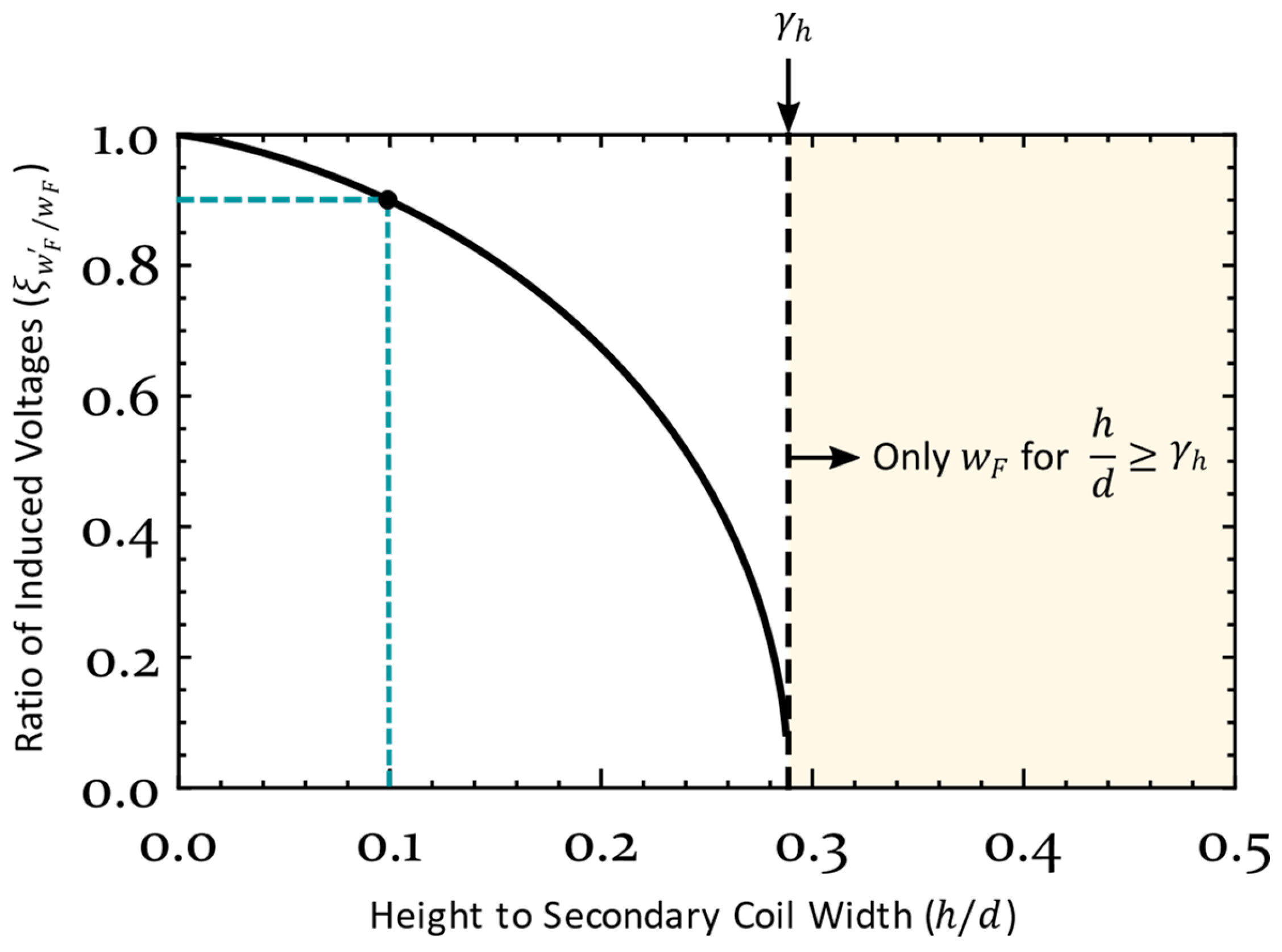
The two possible solutions found, $w_F$ and $w_F^{\prime }$, have different properties concerning the magnitude of voltage that can be induced in each configuration derived. Also, $w_F$ is visibly a larger width than $w_P$, and it is always available as a design option, while $w_F^{\prime }$, when it is defined, is smaller, and associated with lower induced voltages. While both of these values of $D$ will yield a flat response under the center alignment condition, the normalized induced voltage on $s$, under the central alignment condition, will be significant less at $D=w_F^{\prime }$ than at $D=w_F$, except when the ratio $h/d$ is very low (less than 10%), in which case in which the magnitude of the ratio of the induced voltages will be closer to unity (higher than 90%), as shown in Figure 11. However, a too low value of $h/d$ is usually not practical to implement in a real DIWPT application for electric mobility, due to mechanical restrictions on the minimum required air gap.

Figure 11. Condition for the existence of a second smaller width for maximum flatness in the induced voltage.

In summary, although two optimum values were found for a maximum flatness in the induced voltage response, which is a desirable characteristic is some applications, one of them, $w_F^{\prime }$, will only exist if $h/d<28.8\%$. Even then, the induced voltage obtained at $D=w_F^{\prime }$, would be much less than that provided at $D=w_F$, unless $h/d<10\%$, which is likely to be difficult or impractical to implement if the inductive configuration is used for transferring power to terrestrial vehicles. So, the option for the primary coil width of $w_F^{\prime }$ is apparently not as useful for a DIWPT design aiming for lightweight electric mobility as the larger alternative, $w_F$. Thus, in principle, the existence of $w_F^{\prime }$ may be disregarded.

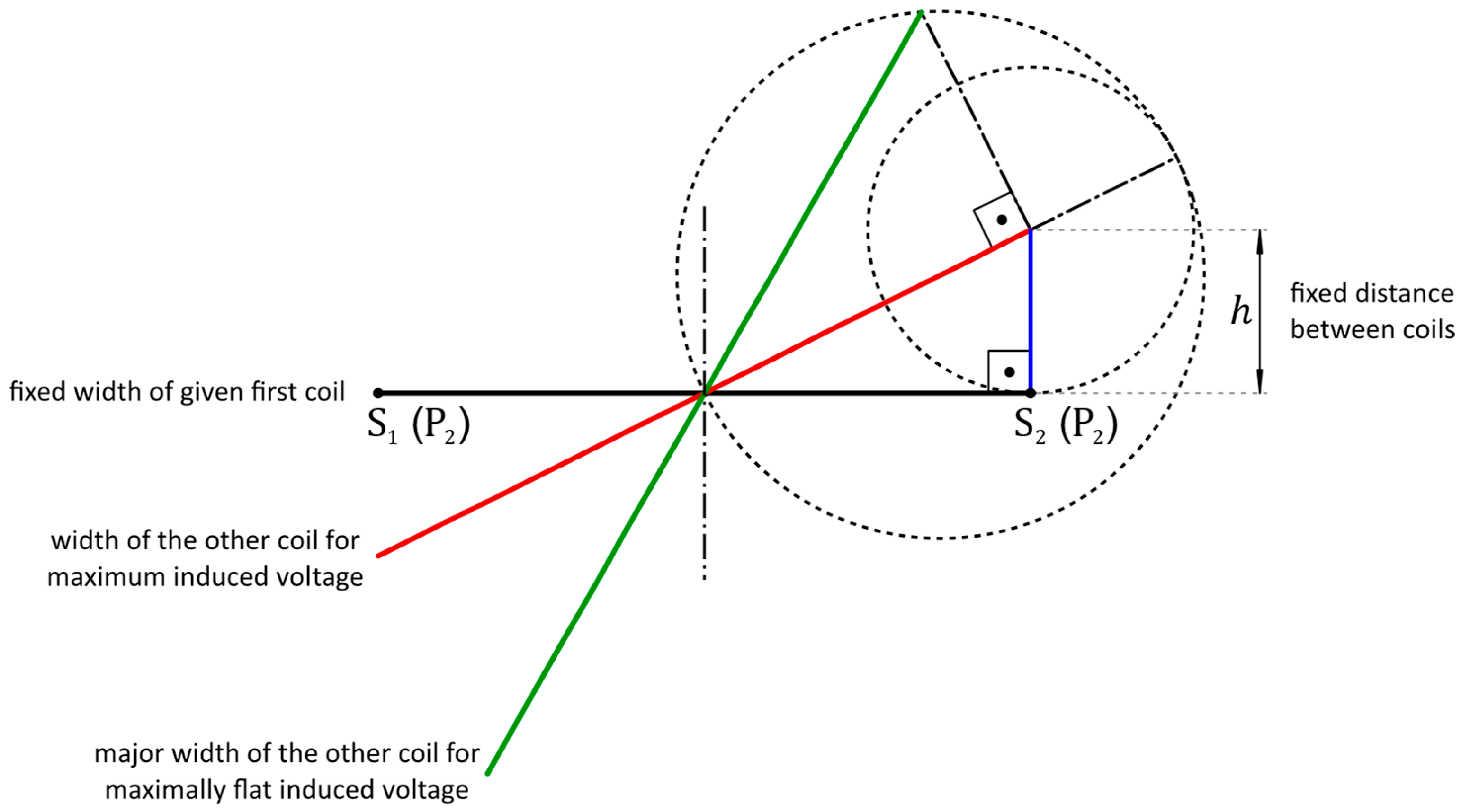
Geometric Interpretation for Theorem 4: A geometrical interpretation is given for the main optimum value $w_F$. Despite not being as straightforward as the geometric construction provided for Theorems 2 and 3, it provides a tool that enhances the visualization, and a more intuitive design of DIWPT configurations using oblong coils, when a maximally flat induced voltage in a secondary coil of given width, is sought.

Figure 12 represents a cross-section of the inductive configuration formed by coils $p$, whose width is a free design parameter, and $s$, of fixed width $d$, given by points $S_1$ and $S_2$, at distance $h$ from the support plane of $p$. For a maximally flat induced voltage, the positioning of the conductors of the primary coil, $w_F$, far apart from each other, is found by first constructing points $P_1$ and $P_2$, such that $\overline{P_1{P}_2}$ is a diameter of a circle also containing $S_1$ and $S_2$, centered at ${\mathtt{C}}_1$, the intersection of the mediatrix of $\overline{S_1{S}_2}$ with the support line at distance $h$ from $\overline{S_1{S}_2}$ ($P_1$ and $P_2$ are the loci for the conductors of $p$ for a maximum induced voltage on $s$, as seen in Theorem 2). Then, point ${\mathtt{H}}_2$ is constructed by making $\overline{P_2{\mathtt{H}}_2}=h$. The intersection of a circle with center at ${\mathtt{C}}_2$ and radius $\overline{{\mathtt{C}}_2{\mathtt{H}}_2}$ with the perpendicular to the support line of the conductors of $p$, drawn from $P_2$, is point ${\mathtt{Z}}_2$. Another circle centered at ${\mathtt{C}}_1$ and drawn with radius $\overline{{\mathtt{C}}_1{\mathtt{Z}}_2}$ will intercept the support line for coil $p$ projections at points ${\mathtt{F}}_1$ and ${\mathtt{F}}_2$, which are the positioning solutions for the conductors of $p$ for a maximally flat induced voltage on $s$. Incidentally, ${\mathtt{F}}_1$ and ${\mathtt{F}}_2$ would be the loci of the conductors of $p$ for maximum voltage on $s$, if $s$, with a distinct width, had its conductors placed at ${\mathtt{Z}}_1$ and ${\mathtt{Z}}_2$, ${\mathtt{Z}}_1$ being the point symmetric to ${\mathtt{Z}}_2$ with respect to the center plane of $s$ that is perpendicular to the support line of $p$.

Figure 12. Geometrical interpretation of Theorem 4.

From this geometric construction, it can be shown that the length of $\overline{{\mathtt{F}}_1{\mathtt{F}}_2}$ is exactly given by the expression derived for $w_F$ (95). For quick estimations of the position of ${\mathtt{F}}_1$ and ${\mathtt{F}}_2$, it can also be verified that

$$d+2h<{ w}_{F }<w_P+2h$$

(97)

3.5. Width of a Secondary Rectangular Coil for a Maximally Flat Induced Voltage by a Given Oblong Primary Coil at a Given Distance from the Secondary Coil, Under Center Alignment Conditions

Theorem 5.

Let $p$ be a stationary, infinitely long filamentary coil p, of fixed width $D$, that is constituted of a single turn of wire carrying a sinusoidal current $I_p$ of constant amplitude and frequency $f_0=2\pi {\omega }_0$; let $s$ be a rectangular coil parallel to $p$ of width $d$ and fixed length $\mathcal{l}$, also constituted of a single turn of filamentary wire and located on a plane that is parallel to the plane that contains $p$, at a fixed distance $h$to that plane. Then, the profile of the normalized voltage $\xi ={\dot{V}}_{ind}/ j\mu f_0{\dot{I}}_p\mathcal{l}$, induced by $p$ on $s$ as a function of the lateral misalignment of $p$ and $s$, is maximally flat in the vicinity of the center alignment condition when the width $d$ of coil s is either equal to $w_F$ or to $w_F^{\prime }$, as given by the following equations and conditions:

$$w_F=\sqrt{w_S^2+4w_{S}h} , h>0$$

(98)

$$w_F^{\prime }=\sqrt{w_S^2-4w_{S}h }, 0<{\displaystyle \frac{h}{d}}<{\gamma }_h$$

(99)

where $w_S$ is the width of $p$ for the maximum induced voltage on s, as in Theorem 3:

$$w_S=\sqrt{D^2+4h^2},$$

(100)

and ${\gamma }_h$ is the optimum $h/D$ ratio for maximum linearity of the induced voltage on $s$ due to a single conductor of $p$, as given by

$${\gamma }_h={\displaystyle \frac{1}{2\sqrt{3}}}$$

(101)

Notably, Theorem 5 can be seen as Theorem 4 with $d$ and $D$ reversed. That is, in Theorem 4 the secondary width is fixed at $d$, and an optimum is sought for the width $D$ of the primary coil, while in Theorem 5 the primary coil has a fixed width $D$, and the problem to be solved is the determination of an optimum secondary width $d$ that will maximize the flatness of the response of the induced voltage as a function of the lateral misalignment of the primary and secondary coils.

Again, likewise to the case of Theorems 2 and 3, there is a duality between Theorems 4 and 5, and the proof of Theorem 5 is based on the same relations and expressions derived for Theorem 4.

Proof of Theorem 5.

Since the inductive configuration and its parameters are equivalent and named exactly as in Theorem 4, the expression for the normalized induced voltage for the present situation is the same as (92), and so are valid expressions (93) and (94). In order to find the optimum, $d$ is then given by the real positive roots of (94), having this time $d$ as the free variable, not $D$ as in the proof of Theorem 4. Since (94) is symmetric with respect to $d$ and $D$, the optimum values for $d$, $w_J$ and $w_J^{\prime }$, are given by

$$w_J=\sqrt{D^2+4h^2+4\sqrt{D^2{h}^2+4h^4}} , h>0, D>0$$

(102)

$$w_J^{\prime }=\sqrt{D^2+4h^2-4\sqrt{D^2{h}^2+4h^4}} , 0<h<D{\displaystyle \frac{1}{2\sqrt{3}}}$$

(103)

It can be recognized from Theorem 3 (77) that $D^2+4h^2=w_S^2$, and from the development of Lemma 1 (32) that ${\gamma }_h=1/2\sqrt{3}$. So, expressions (102) and (103) can be rewritten, respectively, as (99) and (100). □

By analogy to Theorem 4, the geometric evaluation of optimum widths $w_J$ and $w_J^{\prime }$ for a secondary coil $s$ at fixed distance $h$ to a given primary coil with width $D$ will be entirely similar to that shown in Figure 12, but with the drawing up-side down and the location of points $P_1$ and $P_2$, respectively, reversed with $S_1$ and $S_2$.

A general visualization tool for optimum widths of a second coil for the maximum induced voltage (red line segment) and for a maximally flat induced voltage (green line segment) is seen in Figure 13, where the width of the first given coil is represented by the black horizontal line segment and the fixed distance between the two coils. Because of the correspondence of Theorems 3 and 5, respectively, with Theorems 2 and 4, it makes no difference whether the first coil considered is the primary or the secondary coil: the optimum second coil will be always larger than the first coil.

Figure 13. Geometric visualization for the calculation of optimum width coils.

4. Application of Theorems 1 to 5 in DIWPT Design

Considering the possibility of approximating real coils by filamentary windings, for both primary and secondary coils, and provided that their relative velocity is such that the quasi-stationary hypothesis can be applied [34], Theorems 1 to 5 can help the design of DIWPT configurations where the primary coil is an oblong coil and the secondary coil is a rectangular parallel coil at a fixed distance $h$ to the primary coil. This happens because the magnetic field in a cross-section of the primary coil is approximately the same as if the primary coil had infinite length, if the considered cross-section is away from the extremities of the primary coil (by at least one primary coil width of distance or one secondary coil length along the main axis of the primary coil, whichever is larger).

When the secondary coil is compensated, the induced voltage ultimately determines the available power in the secondary coil for a given connected resistive load. In the simplified model considered, the power delivered to the load will be proportional to the squared normalized induced voltage. This is a good reason for the concern in maximizing the induced voltage in practical applications, as established in Theorems 2 and 4.

Alternatively, depending on the circuit design of the secondary coil, the design target might be to have the induced voltage with a flat as possible characteristic, in response to small misalignment variations of the primary and secondary coils, and that is the utility of Theorem 3 and Theorem 5. Theorem 1, on the other hand, provides an analytic method for calculating the induced voltage or the power delivered to $R_L$ as a function of the circuit parameters and the geometry of the coils, allowing the DIWPT design to be refined.

However, in order to fully benefit from the predictions provided by these theorems, the hypothesis of a constant current in the primary coil must hold for a good approximation to be obtained. This will naturally happen if the back-induced voltage from the current secondary coil current is small compared to the voltage established on the primary coil. Noticeably, in DIWPT configurations, where the magnetic coupling coefficient is low, the secondary will likely have more turns than the primary coil, as resulted in our DIWPT application that was developed for e-bikes. It will also happen if the primary circuit is specifically designed to keep the current amplitude constant.

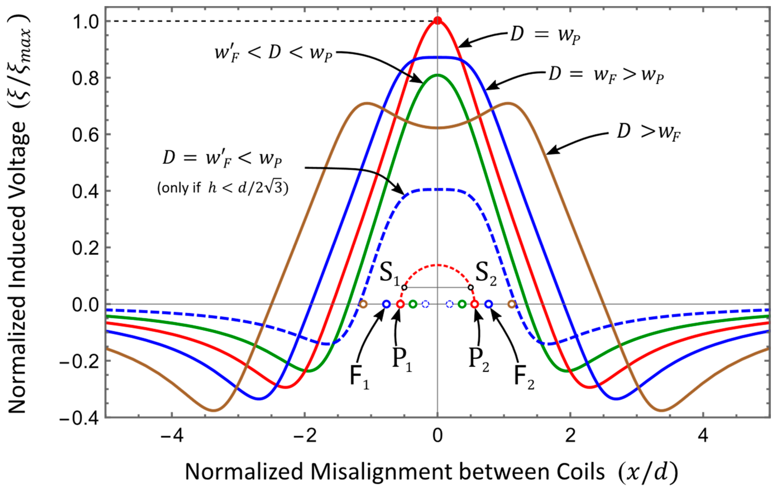
As an illustration of the main mathematical results achieved, the plots of the normalized induced voltage, calculated on basis of the analytical expressions derived for designs with different optimal properties, are exemplified in Figure 14. The configuration corresponds to a given secondary coil with fixed width $d$, at a fixed distance $h$ from a primary coil in which the width $D$ is a parameter of free election by design. The fixed location of the secondary coil is indicated by points $S_1$ and $S_2$, plotted with the vertical axis scale equal to the normalized horizontal scale, differently for the vertical scale for the curves (normalized voltage), for improved perception of the proportions of the geometry in this example, where $h/d$ was set to $1/4$.

Figure 14. Curves of normalized voltage induced on a single-turn rectangular secondary coil by a single-turn oblong primary coil for different primary coil widths, under the conditions of Theorem 1.

In the chart of Figure 14, the induced voltage $\xi$ is normalized by ${\xi }_{max}$ before being plotted, so that the maximum value observed on the vertical axis is one, facilitating the visual comparison of the induced voltage profile of the various configurations. The colors of the curves are in correspondence with the color of the small circles, which represent the location of the conductors of the primary coil that generate each curve. The red curve corresponds to the maximum induced voltage condition, obtained for $D=w_P$, as given by Theorem 2. The two blue curves are the maximally flat induced voltage profiles, obtained for ${D=w}_F$ (continuous blue) and for $D=w_F^{\prime }$ (dashed blue), given by Theorem 4. The green curve is the result of setting the width of the primary coil to a value that is less than $w_P$, but still higher than $w_F^{\prime }$, and the brown curve is an example of a profile generated when the width of the primary coil is larger then $w_F$.

The criterion for a DIWPT design will be strongly dependent on the application. However, in general, the transfer of maximum power for the same primary current is one of the main goals, not only for attaining the required power levels, but also for attaining better efficiency levels, which can be obtained by drawing more power from the same primary current. This is due to the primary losses being strongly related to the square of the rms value of the primary current, which is fixed by hypothesis.

An alternative convenient design goal is to try to keep the amplitude of the induced voltage as constant as possible, while the electric vehicle (secondary coil) harvesting power from the lane (primary coil) drifts laterally around the center of the lane, constantly generating a misalignment input $x$ to the function $\xi$. This property is obtained when $D$ is close to $w_F$, and useful when a DC-DC converter is used to match the load impedance, and the acceptable ratio between the maximum and minimum input to the converter should be kept as low as possible. An in-depth analysis of the application, supported by the tools presented in this section, will lead to the best design choices. In general, unless there is some additional restriction imposed on the width $D$ of the primary coil, there will be no good argument for picking a $D<w_P$ or $D$ much greater than $w_F$.

Concerning electric mobility, although Theorems 3 and 5 provide solutions for optimum geometries of the secondary pick-up coils to be installed on vehicles, the most usual application is to design the primary coil with an optimal width, given a secondary coil of fixed dimensions. This is because whilst the coils should be as large as possible for a good transfer of power, the maximum dimensions of the secondary coil are a priori constrained by the size of the vehicle and mechanical restrictions imposed by the installation of the coil on the vehicle. An example of a graphical construction of the optimum cross-section of an inductive coupling, by the determination of the width $w_F$ of an oblong primary coil (in red) using Theorem 4, given a rectangular secondary coil of width $d$ (in blue), is shown in Figure 15.

Figure 15. Geometric construction of a DIWPT configuration based on oblong primary coils, using Theorem 4.

Once the most favorable dimensions for the coils are fixed, their equivalent circuit parameters, such as inductances and mutual inductance, can be derived and serve as the basis for the circuit design of the primary and the secondary power electronics circuits. Under the hypothesis of concentrated filamentary coil turns, changing the number of turns will vary the self-inductances of the coils and their mutual inductances, providing a means for impedance matching, but the coupling coefficient should remain unaltered if the proximity effect between turns within each coil and the changes in the cross-section of the coils are neglected.

5. Conclusions and Discussion

Five theorems were introduced, aiming to facilitate the design of DIWPT configurations for lightweight vehicular applications, where an oblong coil and a parallel rectangular coil form an air-cored magnetic link, which allows energy to be inductively harvested by wireless power transfer. The first theorem can be seen as a mere manipulation of the basic equations of the mutual inductance between parallel wires, long ago derived [25,35] (pp. 45–47). Theorems 1 and 2 were developed to explain previously developed experimental work, involving the construction and testing of an inductive lane for electric bikes [11,14]. The experimental evaluations of Theorems 3, 4 and 5, which are based on different constraints and desired optimized target behaviors for the induced voltage, are left for future work. Hopefully, all the theorems will serve in other WPT applications where either the primary or the secondary coils are of the oblong type, and the other coil, rectangular, is positioned over the first coil, on a plane that is parallel to that containing the firstly considered oblong coil. In particular, they might find applications in the design of inductive lanes for lower power, lightweight electric vehicles.

Theorems 2 and 3, geometrically interpreted in Figure 10, establish that the width of a first given coil (which can be either the primary or secondary) and the double of the distance separation between the first and the second coil planes form the perpendicular sides of a right triangle where the hypotenuse determines the optimum width of the other coil (respectively, the secondary or primary first coil), maximizing the open secondary induced voltage. Noticeably, the other coil should always be of larger width than that of the first given coil, their size converging to the same value when the distance between them converges to zero, as expected. Hence, these two theorems become more relevant as the distance being imposed between the coils is particularly significant with respect to the dimensions of the first given coil, a typical situation found in DIWPT in electric mobility applications.

Theorems 4 and 5 establish that if a right triangle is formed with the perpendicular sides numerically given by the geometric mean of the optimum width of the second coil for a maximum induced voltage (as calculated by either Theorem 2 or 3) and the double of the distance separation between the first and the second coil planes, then this triangle will have the length of its hypotenuse equal to the width of the primary coil that would yield a maximally flat induced voltage on the secondary coil. In all cases, the theorems only hold when an alternated current of constant amplitude is being imposed on the primary coil.

While the design for maximum induced voltage can help increase both the peak power transferred and the resulting obtained electric efficiency, its flat response to the lateral displacement of the vehicle would simplify the design of the electronic circuitry by diminishing the dynamic input voltage range requirements for the DC-DC converter that, in the secondary coil, regulates the voltage applied to the powertrain. According to the designer’s priorities and, ultimately, to the system requirements, a compromise width for the other coil (which can be either the primary or the secondary coil) can possibly be found between the value given Theorems 2 and 3, and that given by Theorems 4 and 5.

The theorems are expected to be applicable to magnetic link configurations with air gaps constituted by air or other non-conductive materials as long as they exhibit constant and isotropic magnetic permeability.

While inductive lanes for lightweight electric vehicles can have advantages for the overall conservation of energy, as well as for the reduction in both gas emissions and use of natural resources, their adoption is presumed to be a difficult and slow process, not even guaranteed to happen. This is mainly due to the fact that redesigning urban spaces with safe, physically segregated bike lanes normally takes space from other citizens that are neither cyclists nor lightweight transport enthusiasts, and draws resources from other alternative projects and social investments. We also believe that the use of oblong primary coil inductive lanes and lightweight vehicles can perhaps constitute a viable sustainable technical option for the redesign and reconstruction of urban areas that have been greatly damaged, in some cases, completely destroyed and devasted by either natural phenomena or war, either complementing or selectively replacing part of the previously existing heavy-weight vehicular transport network. These circumstances motivated us to try to further disseminate these simple mathematical tools, which are as easy to apply as Pythagoras’ theorem. Hopefully, after being fully validated by experimentation, they might contribute to the design of DIWPT lanes for lightweight electric vehicles, a more sustainable and potentially less expensive technology than that for heavier standard road EVs, which is the current focus of most DIWPT research.