Control for Autonomous Intersection Management Based on Adaptive Control Barrier Function

Abstract

Autonomous intersection management (AIM) is gaining increasing attention due to its crucial role in ensuring safety and efficiency. Various methods have been proposed in the literature to address the AIM problem, including traffic light optimization, connected vehicle optimization based on vehicle-to-anything (V2X) communication technology, and multi-agent autonomous systems. However, each of these approaches has its own limitations, such as parking delays, communication latency, or the lack of guaranteed collision avoidance. This paper presents a novel approach to AIM using adaptive control barrier functions (aCBFs). The proposed aCBF first estimates the power transmission efficiency and incorporates it into the CBF design to ensure collision-free operation. Compared to existing methods, the aCBF approach offers several advantages. Firstly, it eliminates parking delays caused by traffic light systems. Secondly, it can be deployed in intersections with limited network coverage, unlike IoT-based solutions that rely heavily on connectivity. Thirdly, it ensures guaranteed collision-free agent movement at intersections. Specifically, our method guarantees that the minimum distance between agents remains no less than the safe distance at all times, significantly enhancing safety. Furthermore, compared to the TriPField algorithm, our approach achieves a 95% success rate in collision avoidance, demonstrating reliability in autonomous intersection management. The effectiveness of the proposed aCBF-based AIM algorithm has been validated through simulations and experiments with multiple autonomous agent-like robots.

1. Introduction

Every year, numerous traffic accidents occur at intersections due to complicated regulations and improper driver operations. The situation worsens when both human-driven vehicles and autonomous vehicles are present at the intersection. To reduce these accidents, researchers have increasingly focused on the Autonomous Intersection Management (AIM) problem in recent years [1,2,3,4,5,6]. AIM aims to generate collision-free trajectories for vehicles in advance at intersections (refer to Figure 1).

The current AIM approaches can be broadly classified into three categories: traffic light optimization, connected vehicles, and autonomous vehicles [5,6,7,8,9,10,11,12,13,14,15,16,17,18,19,20,21,22,23,24,25,26,27].

1.1. Traffic Light Optimization

Traffic light optimization is still the primary method for managing intersections, but it can result in parking delays. To mitigate these delays, traffic light systems are often optimized based on real-time measurements of traffic density using different sensors installed on the lights [6,7,8,9,10,11].

The AIM system based on traffic light optimzation incorporates various sensor types. In [7], IR sensors were utilized to enable the traffic light system to accurately assess traffic density and adjust the green light duration accordingly, resulting in an adaptive traffic light system. An adaptive traffic signal controller based on reinforcement learning that can learn from high-dimensional sensory data without pre-set parameters was proposed in [16], reducing intersection delays. However, this controller is only effective under low-traffic conditions. Image processing techniques are used in [8,9,10] to analyze traffic density but suffer from poor anti-interference ability and weather sensitivity; accuracy may significantly decrease on rainy or foggy days when cameras cannot capture clear images of intersections. In complex environments, a deep reinforcement learning model was introduced in [11] for controlling the traffic light cycle by analyzing data collected from different sensors to determine traffic density. It should be noted that although these approaches optimize control of the traffic lights, they do not eliminate parking delays at intersections.

1.2. Connected Vehicles (Centralized Control)

Several centralized methods have been proposed in [5,12,13,14,17] to eliminate parking delays. In these methods, traffic management services collect information on all vehicles entering the intersection and compute optimized paths for all vehicles in a centralized manner.

Vehicle-to-anything (V2X) communication technology [12,13] is commonly used as a centralized control technique for intersection management problems. Its main goal is to reduce traffic congestion and prevent accidents, especially in areas prone to accidents like road intersections. A control approach that considers spacing data for both immediate predecessor and successor was proposed under V2X communications environment [17]. However, there are two disadvantages of V2X communication technology in intersection management. First, it is not suitable for large-scale multi-agent systems due to its centralized features, which may cause severe network delays when many vehicles enter an intersection simultaneously. Second, this technology requires high infrastructure requirements such as 5G networks covering the entire intersection and each vehicle having a vehicle-mounted terminal to communicate with the base station.

1.3. Autonomous Vehicles (Decentralized Control)

In order to address the issue of the centralized control method, autonomous vehicles are proposed as a solution to the challenge of connected vehicles being unsuitable for large-scale multi-agent systems. This technology focuses on adjacent vehicles rather than all vehicles at intersections and emphasizes environmental perception and decision-making.

1.3.1. Environmental Perception

In autonomous vehicles, accurate real-time detection and classification of surrounding objects are critical. In [18], researchers propose an object classification method that fuses vision and LiDAR data using a convolutional neural network to obtain informative feature representation for object recognition. In [20], a multi-modal deep learning architecture was suggested to handle RGB-D pictures for object recognition by exploiting the complementary information among different modalities. To enhance nighttime driving scene perception, ref. [21] proposes a method for detecting vehicles while driving at night. Additionally, ref. [22] suggests a perceived model of the environment that classifies four types of moving objects, pedestrians, cyclists, cars, and trucks, improving accuracy in detection and classification for autonomous vehicles.

1.3.2. Decision-Making

Autonomous vehicle technology involves making decisions about the driving strategy based on information such as vehicle position, velocity, direction, lane, and obstacles. At intersections, one of the major maneuvers that requires decision-making for autonomous vehicles is lane-changing [26]. To avoid collisions caused by unreasonable lane-changing, researchers have proposed various methods such as an adaptive fuzzy neural network-based predictor to predict steering angle [23] and a Bayesian network to forecast the probability of lane-changing [28]. As human-driven vehicles will continue to coexist with autonomous vehicles on roads in the future, a decision-making framework resembling human behavior was designed in [24] to reduce discomfort arising from differing driving habits between these vehicle types. It should be noted that there are two disadvantages to autonomous vehicle technology: it requires a lot of training data and cannot guarantee collision-free security due to the complexity of system models and surrounding environments. Therefore, collision avoidance algorithms are crucial for ensuring the safe passage of autonomous vehicles through intersections.

Collision avoidance algorithms have undergone substantial research and development because of their usefulness in many applications [29,30,31,32,33,34,35]. However, many algorithms have major limits when faced with unexpected challenges. Traditional collision avoidance algorithms include the bug algorithm, potential field algorithm, and vector field algorithm [36,37,38,39,40]. Intelligent obstacle avoidance algorithms include the genetic algorithm, fuzzy logic algorithm, and neural network algorithm [41,42,43]. The bug method is the most basic obstacle avoidance algorithm, which involves locating a barrier and wandering around its outline to eliminate it [36,37,38]. The potential field method is a popular approach in robotic motion planning for obstacle avoidance. It represents the environment as a potential field, with the objective exerting an attractive force and impediments exerting repulsive forces [44,45]. The robot navigates by following the resultant force vector, which is the total of various attractive and repulsive forces, directing it toward its destination while avoiding obstacles. However, it can suffer from local minima, when the robot becomes trapped in non-goal locations with zero resultant force, and may exhibit oscillations around obstacles [39]. Therefore, designing a collision avoidance controller for autonomous vehicles to safely navigate intersections is of great importance.

When designing controllers for safety-critical autonomous vehicle operations, such as ensuring that autonomous vehicles pass through intersections without collisions, it is crucial to account for power transmission loss that can significantly impact vehicle performance. These controllers are responsible for dynamically adjusting the vehicle’s control inputs, such as steering angles and acceleration, to ensure safety and efficiency during navigation. However, traditional Control Barrier Function (CBF) approaches may not be suitable for uncertain systems due to their reliance on precise model information. To tackle this challenge, recent studies have introduced adaptive CBF techniques [46,47,48,49]. For example, the online parameter adaptation method in [46] ensures safety, while the strategy outlined in [47] enables operation within larger safe sets. Moreover, the controller utilizing a concurrent learning technique as presented in [48] guarantees exponential convergence of parameter estimation. Additionally, ref. [49] introduces a robust adaptive CBF of higher order, specifically tailored for systems with high-relative-degree safety constraints. However, some existing CBF-based techniques focus on addressing power transmission loss safety issues modeled by input matrix uncertainties that could lead to controllability loss problems [50,51]. Although the Nussbaum gain approach [52] has been suggested to stabilize such issues, systematic methods related to CBF problems are yet to be established.

To overcome the limitations of existing AIM methods, we propose an aCBF-based approach that directly addresses the challenges posed by power transmission loss, ensuring robust safety in autonomous intersection management. Power transmission loss, which results in partial or complete loss of controllability, are a critical issue in AIM scenarios, as they can lead to collisions or delays in vehicle navigation. Our method mitigates these issues through specially designed update laws that adapt to controllability loss, maintaining safety constraints even under fault conditions.

The proposed approach provides the following advantages:

• Adaptive fault compensation —By integrating an adaptive update mechanism, the method effectively compensates for power transmission loss, ensuring safety constraints are upheld even in the presence of controllability loss.
• Decentralized control—The framework operates in a decentralized manner, eliminating the need for traffic lights, reducing vehicle parking delays, and demonstrating scalability in large autonomous systems.
• Computational efficiency—Unlike network-learning-based methods, aCBF-based control does not require pre-training, reducing computational overhead while guaranteeing safety in multi-agent systems.
• Broad applicability—The ability to simultaneously address power transmission loss robustness and broader AIM challenges makes this approach a promising solution for autonomous intersection management.

This paper is organized as follows: CBF preliminaries are covered in Section 2. Section 3 presents the safe adaptive AIM problem and proposes a CBF-based control algorithm for multi-agent systems. Simulations and experiments verifying the algorithm are detailed in Section 4, and conclusions are provided in Section 5.

2. Preliminaries

This section reviews two fundamental methods that underpin our controller design, including the CBF approach and the projection operator for the update law.

2.1. CBF

Consider the following control affine system:

$$\dot{\mathit{x}}=\mathit{f}\left(\mathit{x}\right)+\mathit{g}\left(\mathit{x}\right)\mathit{u},$$

(1)

where $\mathit{x}\in {\mathbb{R}}^n$ is the state, $\mathit{u}\in \mathrm{U}\subset {\mathbb{R}}^m$ is the control input, $\mathit{f}:{\mathbb{R}}^n\to {\mathbb{R}}^n$ and $\mathit{g}:{\mathbb{R}}^n\to {\mathbb{R}}^{n\times m}$ are locally Lipchitz continuous functions. A set $\mathcal{S}$ is called forward controlled invariant with respect to system (1) if for every ${\mathit{x}}_0\in \mathcal{S}$, there exists a control signal $\mathit{u}\left(t\right)$ such that $\mathit{x}(t;t_0,{\mathit{x}}_0)\in \mathcal{S}$ for all $t\ge t_0$, where $\mathit{x}(t;t_0,{\mathit{x}}_0)$ denotes the solution of (1) at time t with initial condition ${\mathit{x}}_0\in {\mathbb{R}}^n$ at time $t_0$.

Consider control system (1) and a set $\mathcal{C}\subset {\mathbb{R}}^n$ defined by

$$\mathcal{C}=\left\{\mathit{x}\in {\mathbb{R}}^n:h\left(\mathit{x}\right)\ge 0\right\},$$

(2)

for a continuously differentiable function $h\left(\mathit{x}\right):{\mathbb{R}}^n\to \mathbb{R}$ that has a relative degree one. The function h is called a (zeroing) CBF if there exists a constant $\gamma >0$ such that

$$\underset{\mathit{u}\in \mathrm{U}}{sup}\left[{\mathcal{L}}_{f}h\left(\mathit{x}\right)+{\mathcal{L}}_{g}h\left(\mathit{x}\right)\mathit{u}+\gamma h\left(\mathit{x}\right)\right]\ge 0,$$

(3)

where ${\mathcal{L}}_{f}h\left(\mathit{x}\right)={\displaystyle \frac{\partial h}{\partial \mathit{x}}}\mathit{f}\left(\mathit{x}\right)$, ${\mathcal{L}}_{g}h\left(\mathit{x}\right)={\displaystyle \frac{\partial h}{\partial \mathit{x}}}\mathit{g}\left(\mathit{x}\right)$ are the Lie derivatives [53]. Given a CBF $h\left(\mathit{x}\right)$, the set of all control values that satisfy (3) for all $\mathit{x}\in {\mathbb{R}}^n$ is defined as $K_{bf}\left(\mathit{x}\right)=\{\mathit{u}\in \mathrm{U}:{\mathcal{L}}_{f}h\left(\mathit{x}\right)+{\mathcal{L}}_{g}h\left(\mathit{x}\right)\mathit{u}+\gamma h\left(\mathit{x}\right)\ge 0\}.$ It was proven in [53] that any Lipschitz continuous controller $\mathit{u}\left(\mathit{x}\right)\in K_{bf}\left(\mathit{x}\right)$ for every $\mathit{x}\in {\mathbb{R}}^n$ will guarantee the forward invariance of $\mathcal{C}$. The provably safe control law is obtained by solving an online quadratic program (QP) problem that includes the control barrier condition as its constraint.

2.2. Projection Operator

To compensate for the power transmission loss in the design of the adaptive controller, the following projection operator is adopted [54]

$$\mathrm{Proj}(\mathit{x},\mathit{y},l)=\left\{\begin{array}{cc}\mathit{y}-l\left(\mathit{x}\right){\displaystyle \frac{\nabla l\left(\mathit{x}\right)\nabla l{\left(\mathit{x}\right)}^{\top }}{{\parallel \nabla l\left(\mathit{x}\right)\parallel }^2}}\mathit{y},\hfill & \mathrm{if}l\left(\mathit{x}\right)>0\wedge {\mathit{y}}^{\top }\nabla l\left(\mathit{x}\right)>0,\hfill \\ \mathit{y},\hfill & \mathrm{otherwise}.\hfill \end{array}\right.$$

Here $\mathit{x}$, $\mathit{y}$ are arbitrary vectors and $l\left(\mathit{x}\right)$ is a convex function defined as

$$l\left(\mathit{x}\right)={\displaystyle \frac{{\mathit{x}}^{\top }\mathit{x}-{\overline{x}}^2}{2\eta \overline{x}+{\eta }^2}},$$

(4)

where $\overline{x}$ and $\eta$ are given positive constants.

Lemma 1.

Given that ${\mathit{x}}^{*}$ is the nominal value of $\mathit{x}$, which may vary from it, if $l\left({\mathit{x}}^{*}\right)\le 0$, one can see that [54]

$${(\mathit{x}-{\mathit{x}}^{*})}^{\top }(\mathrm{Proj}(\mathit{x},\mathit{y},l)-\mathit{y})\le 0.$$

(5)

Lemma 2.

If $\mathit{x}\left(t\right)$ is governed by

$$\dot{\mathit{x}}=\mathrm{Proj}(\mathit{x},\mathit{y},l),$$

(6)

and $l\left(\mathit{x}\right(0\left)\right)\le 1$, one can obtain $l\left(\mathit{x}\right(t\left)\right)\le 1$ for $\forall t\ge 0$, which implies $\parallel \mathit{x}\left(t\right)\parallel \le \overline{x}+\eta$ [54].

3. Controller Design

This section introduces a CBF-based adaptive controller that ensures collision-free motion in uncertain multi-agent systems.

3.1. Control Problem Formalization

The control strategy design employs the following single integrator model for the agents:

$${\dot{\mathit{p}}}_i={\overline{\mathit{u}}}_i,i\in \{1,2,\dots ,n\}.$$

(7)

where n is the number of agents, ${\mathit{p}}_i\in {\mathbb{R}}^2$ represents the state of an agent, ${\overline{\mathit{u}}}_i\in {\mathbb{R}}^2$ denotes the input signal. It is important to note that when actuators do not function as intended (e.g., power transmission loss), the expected performance and stability of the system can be severely compromised [55,56]. To enhance the reliability and performance of systems, control methods must be developed to counteract the impact of power transmission loss, which results in a fault-tolerant control problem. In order to investigate this issue, we introduce a power transmission loss model that considers partial loss of actuator effectiveness [55,56]. The power transmission loss model can be describe as follows:

$${\overline{\mathit{u}}}_i={\theta }_i{\mathit{u}}_i,$$

(8)

where ${\theta }_i>0$ represents the power transmission efficiency of the ith vehicle, and it includes steering power transmission loss, brake power transmission loss, transmission power transmission loss, and so on. Then, (7) can be rearranged as

$${\dot{\mathit{p}}}_i={\theta }_i{\mathit{u}}_i.$$

(9)

where the power transmission efficiency ${\theta }_i$ is assumed to satisfy the following assumptions.

Assumption 1.

To ensure the controllability of system (9), the power transmission efficiency ${\theta }_i$ is assumed to satisfy ${\theta }_i\in [{\alpha }_i,1]$, where ${\alpha }_i$ is a small positive constant $(0<{\alpha }_i<1)$. Without this condition, such as when ${\theta }_i=0$, the system becomes uncontrollable, making the controller design infeasible.

To deal with the AIM problem, in this paper we design a safe adaptive controller for the system (9) based on the CBF technique. The schematic diagram of the CBF in application to the multi-agent system can be seen in Figure 2. To do so, according to Section 2.1, we define a safe set ${\mathcal{C}}_i$ for agent i as

$${\mathcal{C}}_i=\{{\mathit{p}}_i\in {\mathbb{R}}^n\mid h_i\left({\mathit{p}}_i\right)\ge 0\},$$

(10)

where $h_i\left({\mathit{p}}_i\right)$ is a Lipschitz continuous function with a relative degree 1. To avoid collisions, one can design $h_i$ as

$$h_i={\parallel {\mathit{p}}_i-{\mathit{z}}_i\parallel }^2-{\left(2r_{\mathrm{safe}}\right)}^2,$$

(11)

${\mathit{z}}_i$ indicates the position of the nearest neighbor detected within agent i’s sensing range, ${\dot{\mathit{z}}}_i$ is the measurable velocity of this neighbor, and $r_{\mathrm{safe}}$ represents the safety radius that can fit the size of agent i, as shown in Figure 2.

Assumption 2.

The velocity of the detected obstacle ${\dot{z}}_i$ by the ith agent is bounded such that $\parallel {\dot{z}}_i\parallel \le V_z$, where $V_z>0$ is a positive constant.

The control problem can now be stated as follows. Construct the actual input $u_i$ such that the corresponding $p_i\left(t\right)$ resulting from system (9) will stay inside the safety set ${\mathcal{C}}_i$ defined as (10), i.e., $h\left(p_i\left(t\right)\right)\ge 0$ for $\forall t>t_0$, in the presence of uncertainty ${\theta }_i\in [{\alpha }_i,1]$.

To the best of our knowledge, CBF-based safe adaptive controller design for systems with the power transmission loss has not been proposed yet in the literature, which constitutes the novelty of this work.

3.2. A Safe Adaptive Controller Design

Regarding the power transmission loss, setting ${\theta }_i={\theta }_i^{*}+{\displaystyle \frac{1+{\alpha }_i}{2}}$ where ${\alpha }_i>0$ is a small constant, we can see that ${\theta }_i^{*}\in [{\displaystyle \frac{{\alpha }_i-1}{2}},{\displaystyle \frac{1-{\alpha }_i}{2}}]$. By selecting ${\overline{\theta }}_i={\displaystyle \frac{1-{\alpha }_i}{2}}$, we have ${\theta }_i^{*}\in [-{\overline{\theta }}_i,{\overline{\theta }}_i]$. Then, system (9) becomes

$${\dot{p}}_i={\theta }_i^{*}{u}_i+{\displaystyle \frac{1+{\alpha }_i}{2}}{u}_i.$$

(12)

To compensate for the effects of the unknown parameter ${\theta }_i^{*}$ to the control system (12), corresponding update laws ${\widehat{\theta }}_i$ need to be designed for approximating these parameters.

Theorem 1.

By constructing the update law  ${\hat{\theta }}_i$  for the parameter estimation as

$${\dot{\widehat{\theta }}}_i=\mathrm{Proj}\left({\widehat{\theta }}_i,-{\displaystyle \frac{1}{2K_i}}{\left({\displaystyle \frac{\partial h_i}{\partial {\mathit{p}}_i}}\right)}^{\top }{\mathit{u}}_i-{\displaystyle \frac{\mu }{2}}{\widehat{\theta }}_i,l\left({\widehat{\theta }}_i\right)\right),$$

(13)

where $\mu >0$, $l\left({\widehat{\theta }}_i\right)={\displaystyle \frac{{\widehat{\theta }}_i^2-{\overline{\theta }}_i^2}{{\overline{\theta }}_i{\alpha }_i+{({\alpha }_i/2)}^2}}$, $|{\widehat{\theta }}_i\left(0\right)|\le {\displaystyle \frac{1}{2}}$, and $K_i\le {\displaystyle \frac{h_i\left(0\right)}{(|{\widehat{\theta }}_i\left(0\right){|+{\overline{\theta }}_i)}^2}}$, any Lipschitz continuous control ${\mathit{u}}_i\left({\mathit{p}}_i\right)\in K_{bf}({\mathit{p}}_i,{\widehat{\theta }}_i)$ where

$$K_{bf}({\mathit{p}}_i,{\widehat{\theta }}_i)\triangleq \left\{{\mathit{u}}_i\in {\mathbb{R}}^m|\left({\widehat{\theta }}_i+{\displaystyle \frac{1+{\alpha }_i}{2}}\right){\left({\displaystyle \frac{\partial h_i}{\partial {\mathit{p}}_i}}\right)}^{\top }{\mathit{u}}_i-∥{\displaystyle \frac{\partial h_i}{\partial {\mathit{z}}_i}}∥V_z+{\displaystyle \frac{\mu }{2}}\left(h_i-K_i{\overline{\theta }}_i^2\right)\ge 0\right\},$$

(14)

will guarantee the safety of ${\mathcal{C}}_i$ in regard to system (9).

Proof. 

Define ${\overline{h}}_i$ as

$${\overline{h}}_i=h_i-K_i{\tilde{\theta }}_i^2,$$

(15)

where ${\tilde{\theta }}_i={\theta }_i^{*}-{\widehat{\theta }}_i$. To prove Theorem 1, one needs to show that ${\overline{h}}_i\left(t\right)\ge 0$ for $\forall t$, such that $h_i\left(t\right)\ge 0$ for $\forall t$ as required by (10). This property holds if ${\dot{\overline{h}}}_i$ can be expressed in the form of (or larger than) $-\lambda {\overline{h}}_i$, where $\lambda >0$ with ${\overline{h}}_i\left(0\right)\ge 0$.

Following the reconstruction of ${\dot{\overline{h}}}_i$ developed in [51], one obtains

$${\dot{\overline{h}}}_i\ge \left({\widehat{\theta }}_i+{\displaystyle \frac{1+{\alpha }_i}{2}}\right){\left({\displaystyle \frac{\partial h_i}{\partial {\mathit{p}}_i}}\right)}^{\top }{\mathit{u}}_i-{\displaystyle \frac{\mu }{2}}\left(K_i{\overline{\theta }}_i^2\right)-∥{\displaystyle \frac{\partial h_i}{\partial {\mathit{z}}_i}}∥V_z+{\displaystyle \frac{\mu }{2}}{K}_i{\tilde{\theta }}_i^2.$$

(16)

If ${\mathit{u}}_i$ in (16) is selected from (14), the following condition is satisfied

$$\left({\widehat{\theta }}_i+{\displaystyle \frac{1+{\alpha }_i}{2}}\right){\left({\displaystyle \frac{\partial h_i}{\partial {\mathit{p}}_i}}\right)}^{\top }{\mathit{u}}_i-{\displaystyle \frac{\mu }{2}}\left(K_i{\overline{\theta }}_i^2\right)-∥{\displaystyle \frac{\partial h_i}{\partial {\mathit{z}}_i}}∥V_z\ge -{\displaystyle \frac{\mu }{2}}{h}_i,$$

(17)

and thus, in virtue of (15), (16) can be reexpressed as

$${\dot{\overline{h}}}_i\ge -{\displaystyle \frac{\mu }{2}}\left(h_i-K_i{\tilde{\theta }}_i^2\right)=-{\displaystyle \frac{\mu }{2}}{\overline{h}}_i.$$

(18)

In addition, as ${\theta }_i^{*}$ is bounded by ${\overline{\theta }}_i$ respectively, ${\overline{h}}_i\left(0\right)$ satisfies

$$\begin{array}{cc}\hfill {\overline{h}}_i\left(0\right)& =h_i\left(0\right)-K_i{\left({\theta }_i^{*}-{\widehat{\theta }}_i\left(0\right)\right)}^2\ge h_i\left(0\right)-K_i{\left({\overline{\theta }}_i+\left|{\widehat{\theta }}_i\left(0\right)\right|\right)}^2\ge 0.\hfill \end{array}$$

(19)

According to the comparison lemma [57], we know ${\overline{h}}_i\left(t\right)\ge 0$ for $\forall t$, such that $h_i\left(t\right)\ge 0$ for $\forall t$.    □

With the help of Theorem 1, a safe controller is obtained by solving the following CBF-based quadratic programming problem:

$$\begin{array}{cc}\underset{{\mathit{u}}_i^{*}}{min}\hfill & \parallel {\mathit{u}}_i-{\widehat{\mathit{u}}}_i{\parallel }^2\hfill \\ \mathrm{s}.\mathrm{t}.\hfill & \left({\widehat{\theta }}_i+{\displaystyle \frac{1+{\alpha }_i}{2}}\right){\left({\displaystyle \frac{\partial h_i}{\partial {\mathit{p}}_i}}\right)}^{\top }{\mathit{u}}_i-∥{\displaystyle \frac{\partial h_i}{\partial {\mathit{z}}_i}}∥V_z+{\displaystyle \frac{\mu }{2}}\left(h_i-K_i{\overline{\theta }}_i^2\right)\ge 0,\hfill \end{array}$$

where ${\widehat{\theta }}_i$ is updated according to (13), $h_i$ is given in (11), and ${\widehat{\mathit{u}}}_i$ represents a nominal control law that may be unsafe in the intersection. The proposed adaptive CBF (aCBF) controller for the AIM is shown in Figure 3. The entire working process of the proposed algorithm is presented in Algorithm 1.

Algorithm 1: Adaptive CBF-based Controller for AIM

Input: Initial state $p_i\left(0\right)$, initial power transmission efficiency                  ${\theta }_i$, safe set ${\mathcal{C}}_i$, nominal control input ${\widehat{u}}_i$, obstacle velocity                  bound $V_z$. Output: Safe control input $u_i$ ensuring collision-free                 navigation.

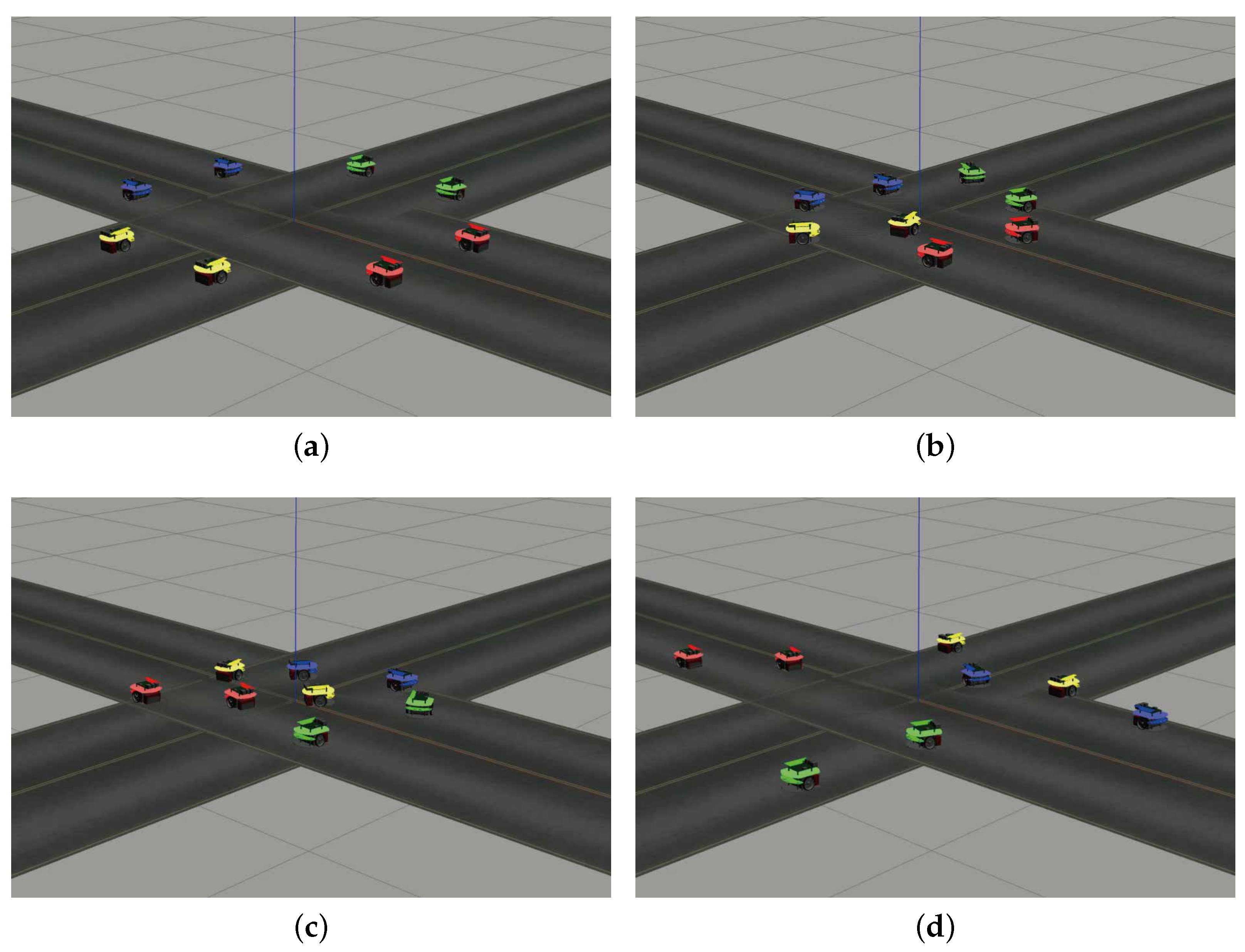
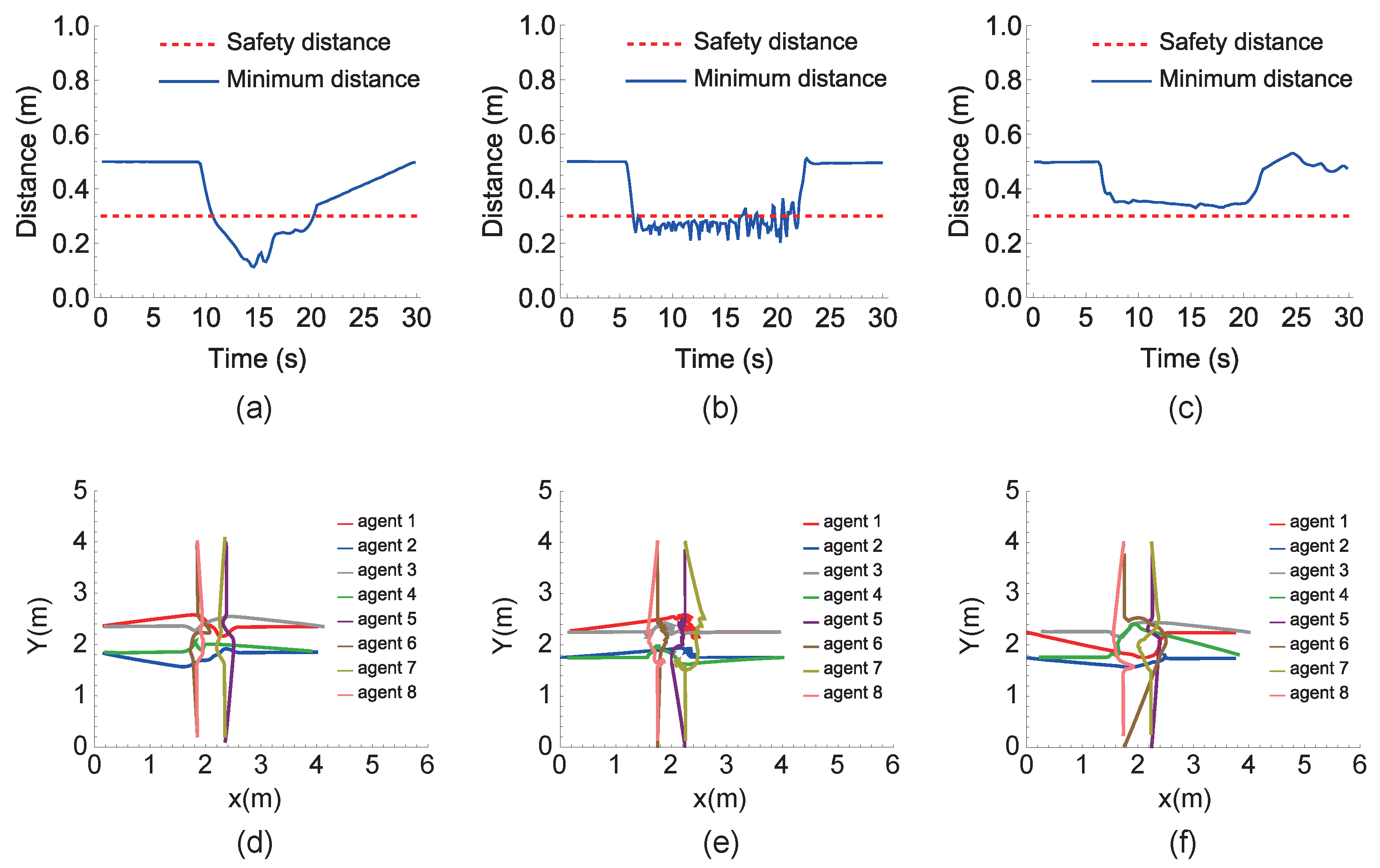
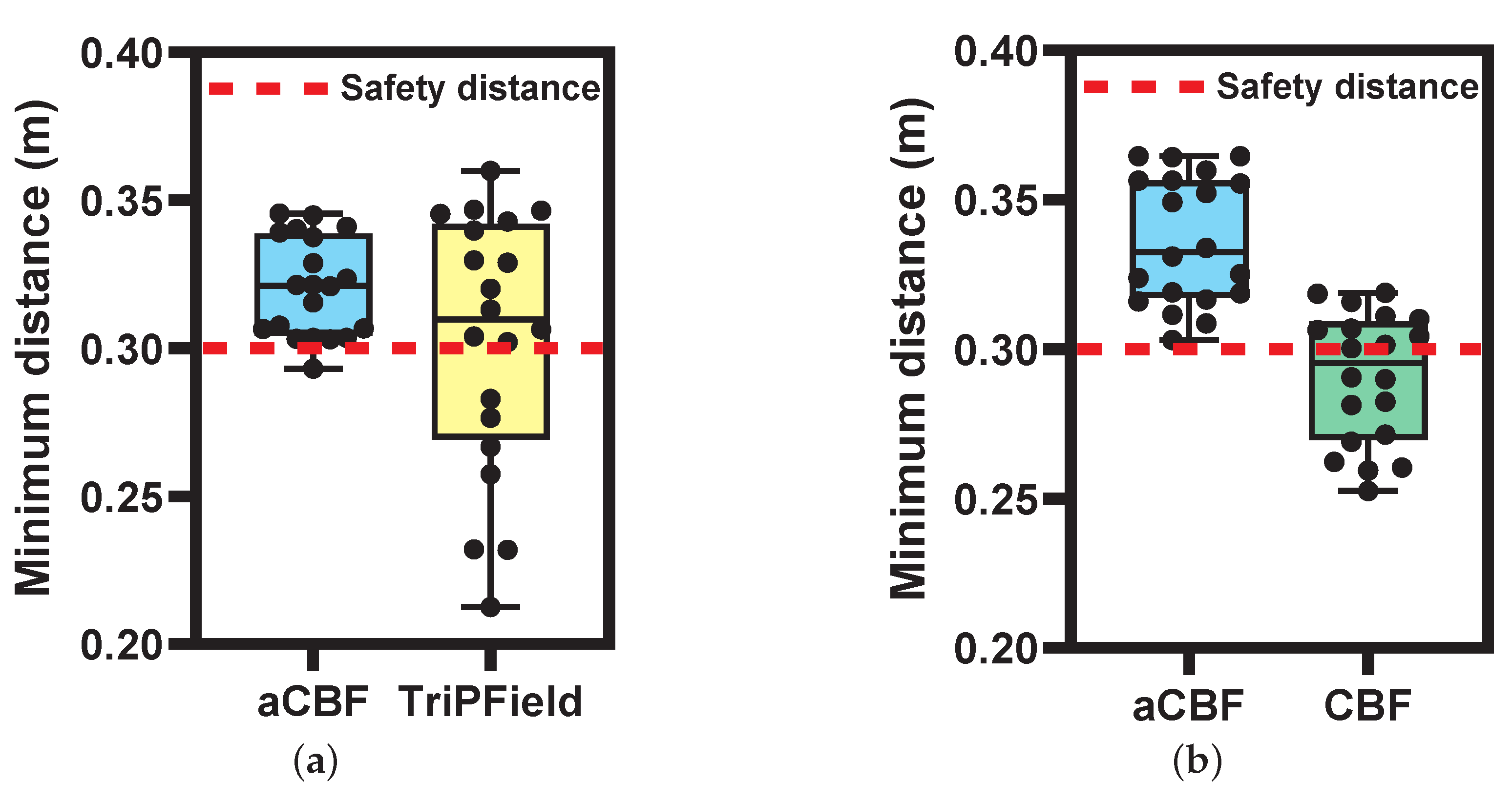
4. Simulations and Experiments

In this section, the proposed controller is verified under simulations and experiments. The raspberry Pi mouse V3 robots (see Figure 4) from RT-Corporation are selected as autonomous vehicles, utilized and controlled by the Robot Operation System (ROS Noetic) in the Ubuntu 20.0.04 LTS environment. The Raspberry Pi mouse V3 robot is a small mobile platform that uses a Raspberry Pi 3B+ as the primary computation board together with a 1000 mAh LiPo battery, four distance sensors, and two four-phase step motors to drive the left and right wheels that operate independently. Since Raspberry Pi mouse robots are differential-drive robots, they can be modeled as unicycles:

$${\dot{x}}_i={\nu }_{i}cos{\varphi }_i$$

(22a)

$${\dot{y}}_i={\nu }_{i}sin{\varphi }_i$$

(22b)

$${\dot{\varphi }}_i={\omega }_i,$$

(22c)

where ${\mathit{p}}_i=(x_i,y_i)$ is the position of robot i, ${\varphi }_i$ its heading, and ${\nu }_i$, ${\omega }_i$ are the translational and angular velocities. Since the CBF algorithm provides desired motions in terms of ${\dot{\mathit{p}}}_i$, we map these onto ${\nu }_i$, ${\omega }_i$ through [58]

$${\nu }_i=\parallel {\dot{\mathit{p}}}_i\parallel ,{\omega }_i=\left[\begin{array}{cc}-sin{\varphi }_i& cos{\varphi }_i\end{array}\right]{\displaystyle \frac{{\dot{\mathit{p}}}_i}{\parallel {\dot{\mathit{p}}}_i\parallel }}.$$

(23)

To verify the feasibility of the proposed CBF-based controller, we conduct simulations in the Gazebo simulator, which is based on the Open Dynamics Engine and Object-Oriented Graphics Rendering Engine. In Gazebo, the robot’s 3D Unified Robotics Description Format (URDF) model, which is a replica of the real robot shown in Figure 4, is utilized for the simulation. The Raspberry Pi mouse’s URDF model can be found on GitHub (version 2.0.0, latest release: 18 November 2024) [59]. Simulations are performed on a desktop featuring an Intel i9-11900F CPU, 64GB RAM, and an NVIDIA RTX 3090 GPU.

4.1. Simulations

In this section, we showcase the effectiveness of the proposed CBF-based controller through simulation. We set up a one-way, two-lane intersection scenario in the Gazebo environment. The scenario is depicted in Figure 5. There are a total of eight robots—yellow, blue, green, and red colored—with two robots of each color in both directions. To simulate a busy intersection, all lane robots enter simultaneously to reach maximum capacity. The objective is for yellow robots to swap positions with green ones and blue robots with red ones without collisions.

The simulation outcomes are displayed in Figure 5 and Figure 8. Figure 5 exhibits snapshots from the simulation, while the initial robot configuration is shown in Figure 5a. As evident from Figure 5b,c, under the proposed aCBF control, each robot maintains safe spacing from others and autonomously plans its path towards the goal position, successfully avoiding collisions as demonstrated by Figure 5d. This collision-free motion is further illustrated in Figure 8c; here, the blue curve represents minimum distances among any two robot pairs which consistently exceed the safety distance $2r_{\mathrm{safe}}=0.3$ m (red dotted curve), ensuring no collisions occur throughout the simulation process. Figure 8f records all the paths of by the eight robots during simulation controlled by the aCBF.

To demonstrate the effectiveness of avoiding collisions at intersections, the results under the three-dimensional potential field (TriPField) method were compared with those under the proposed CBF-based controller. In the same simulation environment, we used the TriPField method to control these eight robots. Under the TriPField method, although each robot autonomously plans its path towards the goal position, as illustrated in Figure 6d, collisions are not completely avoided. As evident from Figure 6b,c, when all robots reach the center of the intersection, there are minor collisions between robots. Figure 8a further illustrates the collisions between robots, showing that at t = 10.5 s, the minimum distance between robots is less than the safety distance. Figure 8d records all paths of the eight robots during the simulation controlled by TriPField. Through comparison, it is concluded that robots controlled by the CBF-based method are safer than those controlled by the TriPField method when passing through the intersection.

To further validate that the aCBF method ensures greater safety compared to the traditional CBF algorithm under power transmission loss, we conducted simulations in the same environment, setting the power transmission efficiency $\theta =0.5$ for each robot. Under the traditional CBF method, although each robot autonomously plans its path to the target position, collisions between robots occur, as shown in Figure 7b. From Figure 7d, it can be observed that a significant collision occurs between the red and yellow vehicles as they move toward their target positions. Figure 8b further illustrates these collisions, revealing that the minimum distance between robots falls below the safety threshold at t = 12 s. Additionally, Figure 8e records the paths of all eight robots controlled by the traditional CBF algorithm during the simulation. A comparison demonstrates that robots controlled by the aCBF method are safer than those controlled by the traditional CBF method when passing through intersections under power transmission loss. Figure 9 presents box plots for two sets of comparative simulations, where each sample represents the minimum distance between any two vehicles in the simulations. Figure 9a compares the aCBF with TriPField, while Figure 9b compares the aCBF with traditional CBF under power transmission loss.

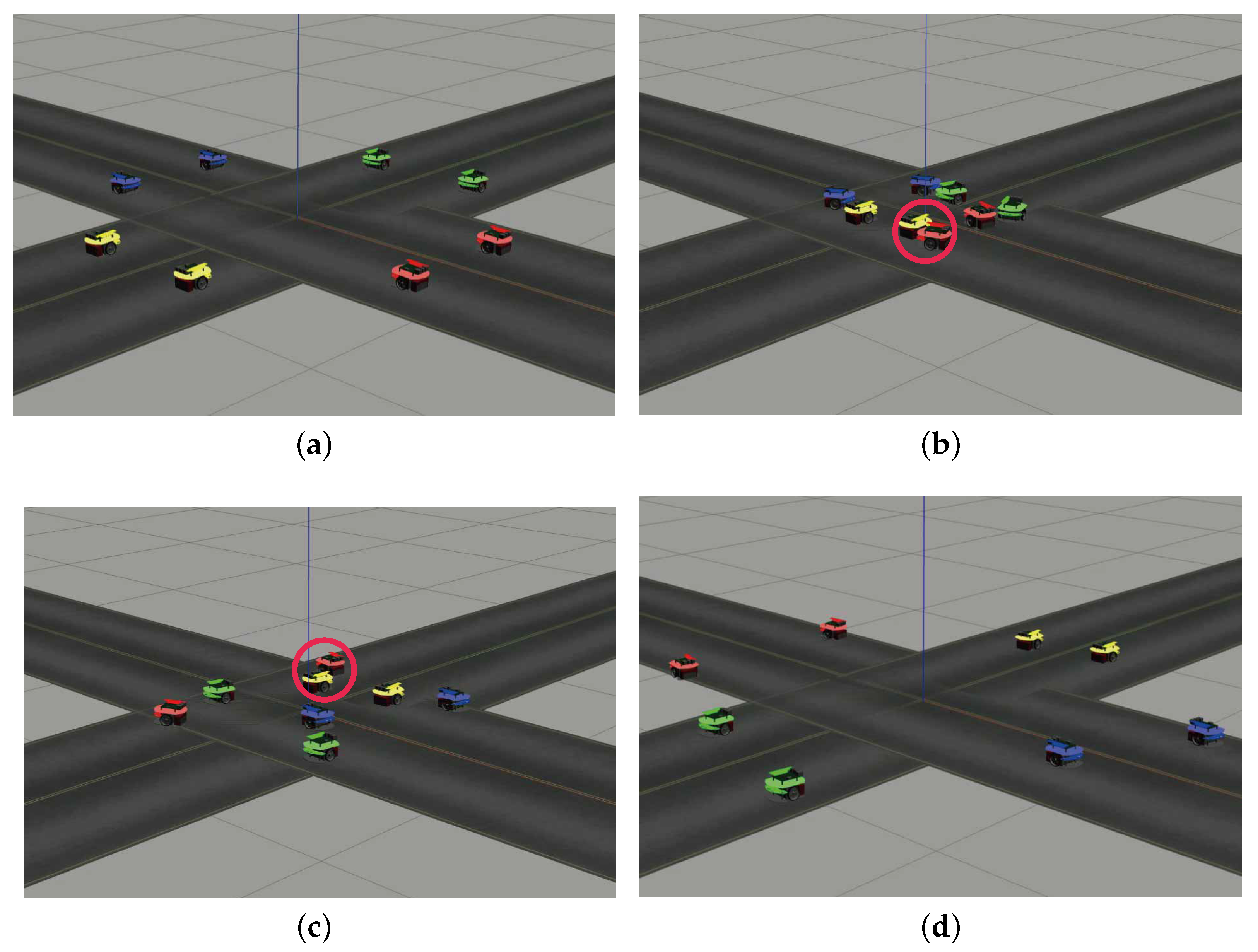
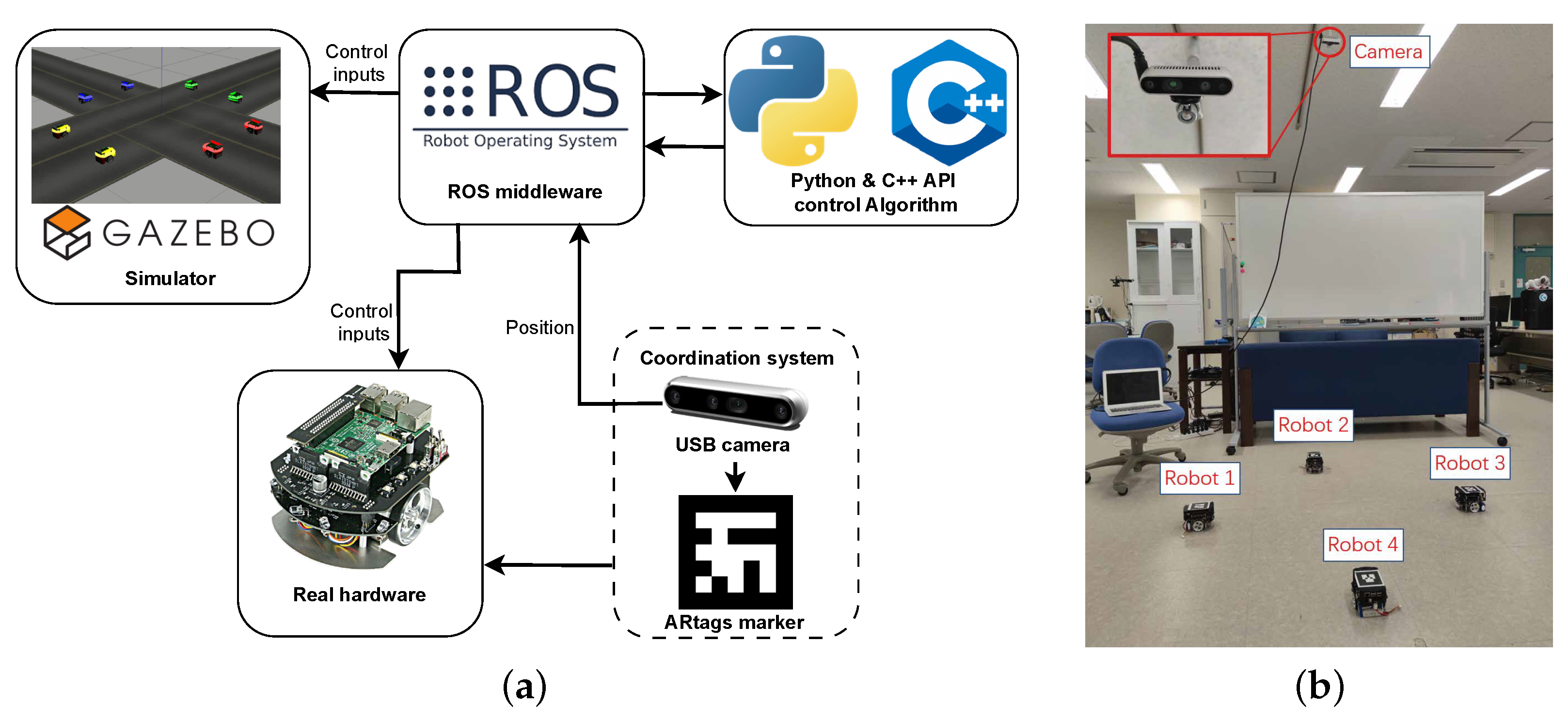
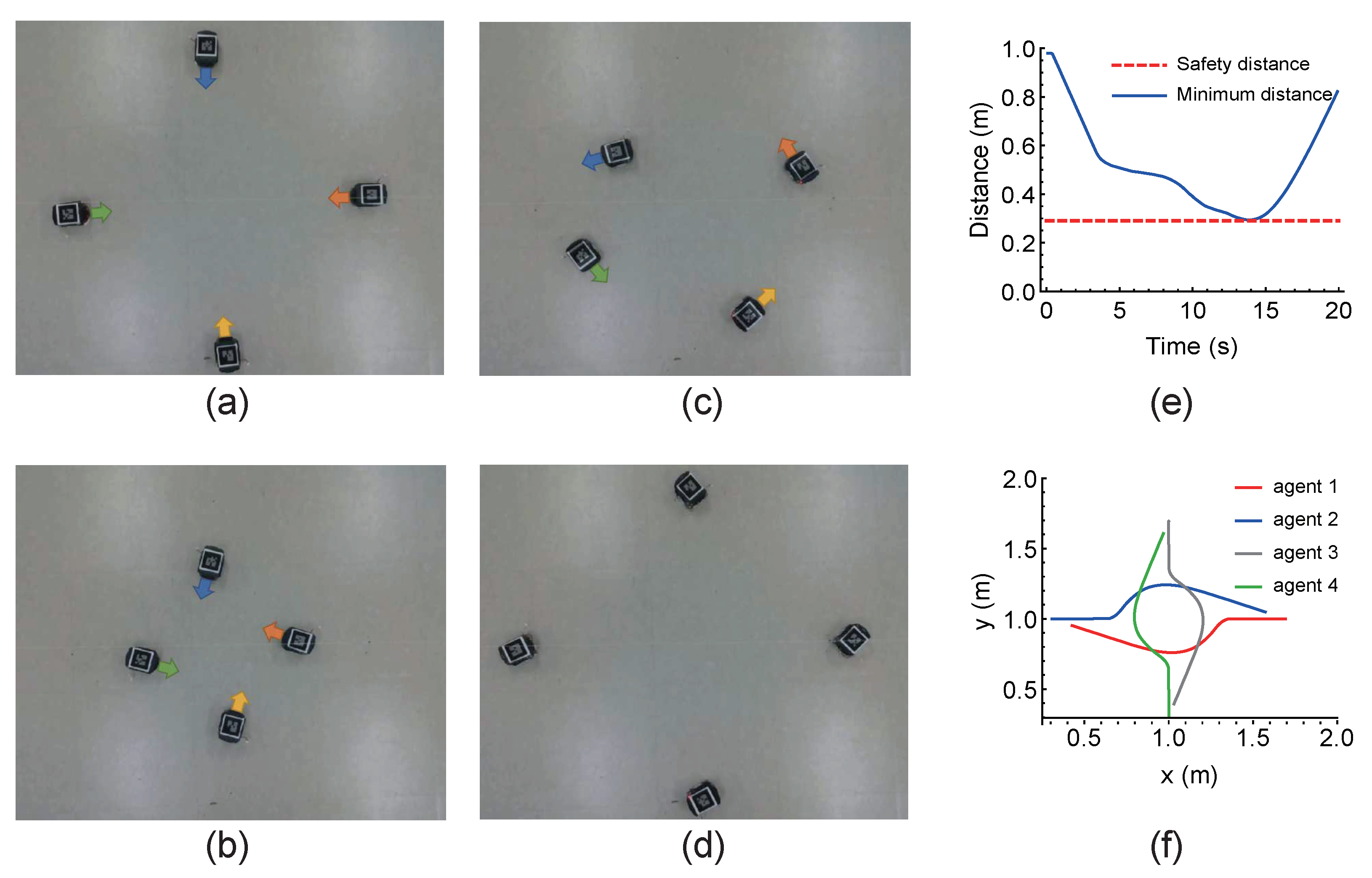
4.2. Experiments

The experimental setup is shown in Figure 10. The hardware and software communication are shown as in Figure 10a. It consists of the Intel Realsense D435 depth camera, computer, and Raspberry Pi mouse robots. The camera is mounted to the ceiling at 2.3 m above the ground and has a field of view that faces downward, as shown in Figure 10b. The USB-C port on the camera is used to connect it to the computer. Each robot has an AR tag on top, which allows the camera to track the robot’s position and orientation. When the camera recognizes the AR tag and records the robot’s position, it transmits this information to the computer through the USB data cable. When the computer receives the information from the camera, the computer generates the control signal and sends it to the robots. The experiment runs on a single desktop computer equipped with an Intel(R) Core(TM) i7-1195G7 CPU and 32GB RAM.

In the experiments, we set up a one-way, single-lane intersection scenario, shown in Figure 11. There are four robots involved, with one robot positioned on each lane facing opposite directions. We synchronize the entry of the robots from both lanes into the center simultaneously. The objective of the experiment is for the robot marked with a yellow arrow to swap positions with the one marked with a blue arrow, and for the robot indicated by a green arrow to exchange places with the one pointed out by an orange arrow without any collision.

The AIM experiment results are presented in Figure 11. It displays the top-view snapshots from the experiment, including the initial robot configuration shown in Figure 11a. Figure 11b,c demonstrate that each robot, under aCBF control, maintains a safe distance from others and navigates autonomously towards the goal position. In Figure 11d, all robots successfully cross the intersection without collisions occurring. This collision-free movement is further illustrated in Figure 11e, where the blue curve represents the minimum distance between any pair of robots, exceeding the safety threshold $2r_{\mathrm{safety}}$ = 0.3 m indicated by the red curve throughout the entire experiment duration, ensuring no collisions took place. Figure 11f depicts all robots’ trajectories during the experiment period.

5. Conclusions

In this paper, we have presented an innovative approach for Autonomous Intersection Management (AIM) utilizing adaptive control barrier functions (aCBFs). The proposed method effectively addresses the critical challenges of safety and efficiency in managing intersections with both static obstacles and autonomous vehicles. By incorporating adaptive fault compensation, the aCBF framework ensures robust performance even in the presence of power transmission loss, making it a reliable and scalable solution for autonomous intersection management.

Through extensive simulations, our results demonstrate that the aCBF significantly outperforms existing multi-agent collision avoidance algorithms in ensuring safe vehicle navigation. In comparative studies, the aCBF achieves a 95% collision avoidance rate, whereas the TriPField algorithm only maintains 65%. Furthermore, when power transmission loss occurs, the aCBF still ensures 100% collision avoidance, while the traditional CBF only achieves 45%. This highlights the superiority of the aCBF in ensuring intersection safety under real-world uncertainties. This work contributes to advancing robust and adaptive safety mechanisms in autonomous intersection management, offering a promising solution for large-scale deployment in intelligent traffic management.

Despite these advantages, the current approach assumes that all vehicles entering the intersection are autonomous and controlled by the aCBF. However, in the foreseeable future, mixed traffic scenarios will emerge, where autonomous vehicles coexist with human-driven vehicles. Human drivers exhibit unpredictable behaviors, introducing additional challenges for intersection management. To further enhance the safety and adaptability of our algorithm, future work will explore the integration of machine learning techniques, such as human behavior prediction models and reinforcement learning, to anticipate human driving behaviors and proactively adjust aCBF-based control strategies.

References

- Dresner, K.; Stone, P. A multiagent approach to autonomous intersection management. J. Artif. Intell. Res. 2008, 31, 591–656. [Google Scholar] [CrossRef]
- Filocamo, B.; Alonso Ruiz, J.; Sotelo, M.A. Efficient management of road intersections for automated vehicles—The FRFP system applied to the various types of intersections and roundabouts. Appl. Sci. 2019, 10, 316. [Google Scholar] [CrossRef]
- Carlino, D.; Boyles, S.D.; Stone, P. Auction-Based Autonomous Intersection Management. In Proceedings of the 16th International IEEE Conference on Intelligent Transportation Systems (ITSC 2013), The Hague, The Netherlands, 6–9 October 2013; Volume 16, pp. 529–534. [Google Scholar]
- Namazi, E.; Li, J.; Lu, C. Intelligent intersection management systems considering autonomous vehicles: A systematic literature review. IEEE Access 2019, 7, 91946–91965. [Google Scholar] [CrossRef]
- Bian, Y.; Li, S.E.; Ren, W.; Wang, J.; Li, K.; Liu, H.X. Cooperation of multiple connected vehicles at unsignalized intersections: Distributed observation, optimization, and control. IEEE Trans. Ind. Electron. 2019, 67, 10744–10754. [Google Scholar] [CrossRef]
- Noh, S. Decision-making framework for autonomous driving at road intersections: Safeguarding against collision, overly conservative behavior, and violation vehicles. IEEE Trans. Ind. Electron. 2018, 66, 3275–3286. [Google Scholar] [CrossRef]
- Ghazal, B.; ElKhatib, K.; Chahine, K.; Kherfan, M. Smart Traffic Light Control System. In Proceedings of the Third International Conference on Electrical, Electronics, Computer Engineering and Their Applications (EECEA), Beirut, Lebanon, 21–23 April 2016; Volume 3, pp. 140–145. [Google Scholar]
- Vidhya, K.; Banu, A.B. Density-based traffic signal system. Int. J. Innov. Res. Sci. Eng. Technol. 2014, 3, 2218–2222. [Google Scholar]
- Monika, G.; Kalpana, N.; Gnanasundari, P. An intelligent automatic traffic light controller using embedded systems. Int. J. Innov. Res. Sci. Eng. Technol. 2015, 4, 19–27. [Google Scholar]
- Chen, Y.L.; Wu, B.F.; Huang, H.Y.; Fan, C.J. A real-time vision system for nighttime vehicle detection and traffic surveillance. IEEE Trans. Ind. Electron. 2010, 58, 2030–2044. [Google Scholar] [CrossRef]
- Liang, X.; Du, X.; Wang, G.; Han, Z. A deep reinforcement learning network for traffic light cycle control. IEEE Trans. Veh. Technol. 2019, 68, 1243–1253. [Google Scholar] [CrossRef]
- Hobert, L.; Festag, A.; Llatser, I.; Altomare, L.; Visintainer, F.; Kovacs, A. Enhancements of V2X communication in support of cooperative autonomous driving. IEEE Commun. Mag. 2015, 53, 64–70. [Google Scholar] [CrossRef]
- Dorrell, D.; Vinel, A.; Cao, D. Connected vehicles—Advancements in vehicular technologies and informatics. IEEE Trans. Ind. Electron. 2015, 62, 7824–7826. [Google Scholar] [CrossRef]
- Lin, P.; Liu, J.; Jin, P.J.; Ran, B. Autonomous vehicle-intersection coordination method in a connected vehicle environment. IEEE Intell. Transp. Syst. Mag. 2017, 9, 37–47. [Google Scholar] [CrossRef]
- Isele, D.; Cosgun, A.; Fujimura, K. Analyzing knowledge transfer in deep Q-networks for autonomously handling multiple intersections. arXiv 2017, arXiv:1705.01197. [Google Scholar]
- Shabestary, S.M.A.; Abdulhai, B. Deep learning vs. discrete reinforcement learning for adaptive traffic signal control. Proc. Int. Conf. Intell. Transp. Syst. 2018, 21, 286–293. [Google Scholar]
- Seiler, P.; Pant, A.; Hedrick, K. Disturbance propagation in vehicle strings. IEEE Trans. Autom. Control 2004, 49, 1835–1842. [Google Scholar] [CrossRef]
- Gao, H.; Cheng, B.; Wang, J.; Li, K.; Zhao, J.; Li, D. Object classification using CNN-based fusion of vision and LIDAR in autonomous vehicle environment. IEEE Trans. Ind. Inform. 2018, 14, 4224–4231. [Google Scholar] [CrossRef]
- Bai, Y.; Wang, Y.; Xiong, X.; Svinin, M.; Magid, E. Adaptive Multi-Agent Control with Dynamic Obstacle Avoidance in a Limited Region. In Proceedings of the 2022 American Control Conference (ACC), Atlanta, GA, USA, 8–10 June 2022; IEEE: Piscataway, NJ, USA, 2022; pp. 4695–4700. [Google Scholar]
- Wang, A.; Lu, J.; Cai, J.; Cham, T.J.; Wang, G. Large-margin multi-modal deep learning for RGB-D object recognition. IEEE Trans. Multimedia 2015, 17, 1887–1898. [Google Scholar] [CrossRef]
- Kosaka, N.; Ohashi, G. Vision-based nighttime vehicle detection using CenSurE and SVM. IEEE Trans. Intell. Transp. Syst. 2015, 16, 2599–2608. [Google Scholar] [CrossRef]
- Chavez-Garcia, R.O.; Aycard, O. Multiple sensor fusion and classification for moving object detection and tracking. IEEE Trans. Intell. Transp. Syst. 2015, 17, 525–534. [Google Scholar] [CrossRef]
- Tang, J.; Liu, F.; Zhang, W.; Ke, R.; Zou, Y. Lane-changes prediction based on adaptive fuzzy neural network. Expert Syst. Appl. 2018, 91, 452–463. [Google Scholar] [CrossRef]
- Hang, P.; Lv, C.; Xing, Y.; Huang, C.; Hu, Z. Human-like decision making for autonomous driving: A noncooperative game theoretic approach. IEEE Trans. Intell. Transp. Syst. 2020, 22, 2076–2087. [Google Scholar] [CrossRef]
- Bai, Y.; Wang, Y.; Svinin, M.; Magid, E.; Sun, R. Adaptive multi-agent coverage control with obstacle avoidance. IEEE Control Syst. Lett. 2021, 6, 944–949. [Google Scholar] [CrossRef]
- Wang, W.; Qie, T.; Yang, C.; Liu, W.; Xiang, C.; Huang, K. An intelligent lane-changing behavior prediction and decision-making strategy for an autonomous vehicle. IEEE Trans. Ind. Electron. 2021, 69, 2927–2937. [Google Scholar] [CrossRef]
- Mihály, A.; Farkas, Z.; Gáspár, P. Multicriteria autonomous vehicle control at non-signalized intersections. Appl. Sci. 2020, 10, 7161. [Google Scholar] [CrossRef]
- Rehder, T.; Muenst, W.; Louis, L.; Schramm, D. Learning lane change intentions through lane contentedness estimation from demonstrated driving. In Proceedings of theIEEE 19th International Conference on Intelligent Transportation Systems (ITSC), Rio de Janeiro, Brazil, 1–4 November 2016; pp. 893–898. [Google Scholar]
- Chen, J.; Zhou, Y.; Lv, Q.; Deveerasetty, K.K.; Dike, H.U. A review of autonomous obstacle avoidance technology for multi-rotor UAVs. In Proceedings of the IEEE International Conference on Information and Automation (ICIA), Wuyishan, China, 11–13 August 2018; pp. 244–249. [Google Scholar]
- Ames, A.D.; Xu, X.; Grizzle, J.W.; Tabuada, P. Control barrier function based quadratic programs for safety critical systems. IEEE Trans. Autom. Control 2017, 62, 3861–3876. [Google Scholar] [CrossRef]
- Yan, H.; Zhu, Q.; Zhang, Y.; Li, Z.; Du, X. An obstacle avoidance algorithm for unmanned surface vehicle based on a star and velocity-obstacle algorithms. In Proceedings of the 2022 IEEE 6th Information Technology and Mechatronics Engineering Conference (ITOEC), Chongqing, China, 4–6 March 2022; Volume 6, pp. 77–82. [Google Scholar]
- Peng, Y.; Qu, D.; Zhong, Y.; Xie, S.; Luo, J.; Gu, J. Obstacle detection and obstacle avoidance algorithm based on 2-D RPLIDAR. In Proceedings of the IEEE International Conference on Parallel & Distributed Processing with Applications, Big Data & Cloud Computing, Sustainable Computing & Communications, Social Computing & Networking (ISPA/BDCloud/SocialCom/SustainCom), New York City, NY, USA, 30 September–3 October 2021; pp. 1–4. [Google Scholar]
- Kim, J.C.; Pae, D.S.; Lim, M.T. Obstacle avoidance path planning algorithm based on model predictive control. In Proceedings of the 18th IEEE International Conference on Control, Automation and Systems (ICCAS), Pyeong Chang, Republic of Korea, 17–20 October 2018; pp. 141–143. [Google Scholar]
- Jia, F.; Liu, X.; Wu, J.; Shi, Y.; Xu, F.; Zhang, Z. Research on multi-AGV autonomous obstacle avoidance strategy based on improved A* algorithm. In Proceedings of the 2018 25th International Conference on Mechatronics and Machine Vision in Practice (M2VIP), Stuttgart, Germany, 20–22 November 2018; pp. 1–6. [Google Scholar]
- Song, X. Research and design of robot obstacle avoidance strategy based on multisensor and fuzzy control. In Proceedings of the IEEE 2nd International Conference on Data Science and Computer Application (ICDSCA), Dalian, China, 28–30 October 2022; pp. 930–933. [Google Scholar]
- Ng, S.Y.; Ahmad, N.S. A bug-inspired algorithm for obstacle avoidance of a nonholonomic wheeled mobile robot with constraints. In Intelligent Computing, Proceedings of the 2019 Computing Conference, London, UK, 16–17 July 2019; Springer International Publishing: Berlin/Heidelberg, Germany, 2019; Volume 2, pp. 1235–1246. [Google Scholar]
- Sivaranjani, S.; Nandesh, D.A.; Gayathri, K.; Ramanathan, R. An investigation of bug algorithms for mobile robot navigation and obstacle avoidance in two-dimensional unknown static environments. In Proceedings of the International Conference on Communication information and Computing Technology (ICCICT), Mumbai, India, 25–27 June 2021; pp. 1–6. [Google Scholar]
- Cichosz, C.; Gurocak, H. Collision avoidance in human-cobot work cell using proximity sensors and modified bug algorithm. In Proceedings of the 2022 10th IEEE International Conference on Control, Mechatronics and Automation (ICCMA), Belval, Luxembourg, 9–12 November 2022; pp. 53–59. [Google Scholar]
- Chen, Y.-S.M.J.-Q.Y.; Luo, G.-C.; Su, X.-L. UAV path planning using artificial potential field method updated by optimal control theory. Int. J. Syst. Sci. 2016, 47, 1407–1420. [Google Scholar] [CrossRef]
- Ulrich, I.; Borenstein, J. VFH+: Reliable obstacle avoidance for fast mobile robots. In Proceedings of the IEEE International Conference on Robotics and Automation, Leuven, Belgium, 20–20 May 1998; Volume 2, pp. 1572–1577. [Google Scholar]
- Srinivasan, D.; Cheu, R.; Poh, Y.; Ng, A. Development of an intelligent technique for traffic network incident detection. Eng. Appl. Artif. Intell. 2000, 13, 311–322. [Google Scholar] [CrossRef]
- Perez-D’Arpino, C.; Medina-Melendez, W.; Guzman, J.; Fermin, L.; Fernandez-Lopez, G. Fuzzy logic based speed planning for autonomous navigation under velocity field control. In Proceedings of the 2009 IEEE International Conference on Mechatronics, Malaga, Spain, 14–17 April 2009; pp. 1–6. [Google Scholar]
- He, R.W.R.; Zhang, Q. UAV autonomous collision avoidance approach. Automatika 2017, 58, 195–204. [Google Scholar] [CrossRef]
- Liu, C.; Zhai, L.; Zhang, X. Research on local real-time obstacle avoidance path planning of unmanned vehicle based on improved artificial potential field method. In Proceedings of the 2022 6th CAA International Conference on Vehicular Control and Intelligence (CVCI), Nanjing, China, 28–30 October 2022; pp. 1–6. [Google Scholar]
- Lu, S.X.; Li, E.; Guo, R. An obstacles avoidance algorithm based on improved artificial potential field. In Proceedings of the 2020 IEEE International Conference on Mechatronics and Automation (ICMA), Beijing, China, 2–5 August 2020; pp. 425–430. [Google Scholar]
- Taylor, A.J.; Ames, A.D. Adaptive safety with control barrier functions. In Proceedings of the 2020 American Control Conference (ACC), Denver, CO, USA, 1–3 July 2020; pp. 1399–1405. [Google Scholar]
- Lopez, B.T.; Slotine, J.J.E.; How, J.P. Robust adaptive control barrier functions: An adaptive and data-driven approach to safety. IEEE Control Syst. Lett. 2020, 5, 1031–1036. [Google Scholar] [CrossRef]
- Isaly, A.; Patil, O.S.; Sanfelice, R.G.; Dixon, W.E. Adaptive safety with multiple barrier functions using integral concurrent learning. In Proceedings of the 2021 American Control Conference (ACC), New Orleans, LA, USA, 25–28 May 2021; pp. 3719–3724. [Google Scholar]
- Cohen, M.H.; Belta, C. High order robust adaptive control barrier functions and exponentially stabilizing adaptive control Lyapunov functions. arXiv 2022, arXiv:2203.01999. [Google Scholar]
- Bechlioulis, C.P.; Rovithakis, G.A. Robust adaptive control of feedback linearizable MIMO nonlinear systems with prescribed performance. IEEE Trans. Autom. Control 2008, 53, 2090–2099. [Google Scholar] [CrossRef]
- Bai, Y.; Wang, Y.; Xiong, X.; Song, J.; Svinin, M. Safe adaptive multi-agent coverage control. IEEE Control Syst. Lett. 2023, 7, 3217–3222. [Google Scholar] [CrossRef]
- Liu, Y.J.; Tong, S. Barrier Lyapunov functions for Nussbaum gain adaptive control of full state constrained nonlinear systems. Automatica 2017, 76, 143–152. [Google Scholar] [CrossRef]
- Xu, X.; Tabuada, P.; Ames, A.D.; Grizzle, J.W. Robustness of control barrier functions for safety critical control. Proc. IFAC Conf. Anal. Des. Hybrid Syst. 2015, 48, 54–61. [Google Scholar]
- Lavretsky, E.; Gibson, T.E. Projection operator in adaptive systems. arXiv 2011, arXiv:1112.4232. [Google Scholar]
- Ye, D.; Yang, G.-H. Adaptive fault-tolerant tracking control against actuator faults with application to flight control. IEEE Trans. Control Syst. Technol. 2006, 14, 1088–1096. [Google Scholar] [CrossRef]
- Liu, Z.; Yuan, C.; Zhang, Y. Active fault-tolerant control of unmanned quadrotor helicopter using linear parameter varying technique. J. Intell. Robot. Syst. 2017, 88, 415–436. [Google Scholar] [CrossRef]
- Khalil, H.K. Nonlinear Systems, 3rd ed.; Prentice Hall: Upper Saddle River, NJ, USA, 2002. [Google Scholar]
- Lee, S.G.; Diaz-Mercado, Y.; Egerstedt, M. Multirobot Control Using Time-Varying Density Functions. IEEE Trans. Robot. 2015, 31, 489–493. [Google Scholar] [CrossRef]
- Raspimouse_description. Available online: https://github.com/rt-net/raspimouse_description.git (accessed on 5 July 2024).
- Ji, Y.; Ni, L.; Zhao, C.; Lei, C.; Du, Y.; Wang, W. TriPField: A 3D Potential Field Model and Its Applications to Local Path Planning of Autonomous Vehicles. IEEE Trans. Intell. Transp. Syst. 2023, 24, 3541–3554. [Google Scholar] [CrossRef]
- Liu, J.; Yang, J.; Mao, J.; Zhu, T.; Xie, Q.; Li, Y.; Wang, X.; Li, S. Flexible active safety motion control for robotic obstacle avoidance: A CBF-guided MPC approach. IEEE Robot. Autom. Lett. 2025, 10, 2686–2693. [Google Scholar] [CrossRef]
Disclaimer/Publisher’s Note: The statements, opinions and data contained in all publications are solely those of the individual author(s) and contributor(s) and not of MDPI and/or the editor(s). MDPI and/or the editor(s) disclaim responsibility for any injury to people or property resulting from any ideas, methods, instructions or products referred to in the content. |
© 2025 by the authors. Licensee MDPI, Basel, Switzerland. This article is an open access article distributed under the terms and conditions of the Creative Commons Attribution (CC BY) license (https://creativecommons.org/licenses/by/4.0/).
Share and Cite
Song, J.; Svinin, M.; Wakamiya, N. Control for Autonomous Intersection Management Based on Adaptive Control Barrier Function. Appl. Sci. 2025, 15, 2315. https://doi.org/10.3390/app15052315
Song J, Svinin M, Wakamiya N. Control for Autonomous Intersection Management Based on Adaptive Control Barrier Function. Applied Sciences. 2025; 15(5):2315. https://doi.org/10.3390/app15052315
Chicago/Turabian StyleSong, Jie, Mikhail Svinin, and Naoki Wakamiya. 2025. "Control for Autonomous Intersection Management Based on Adaptive Control Barrier Function" Applied Sciences 15, no. 5: 2315. https://doi.org/10.3390/app15052315
APA StyleSong, J., Svinin, M., & Wakamiya, N. (2025). Control for Autonomous Intersection Management Based on Adaptive Control Barrier Function. Applied Sciences, 15(5), 2315. https://doi.org/10.3390/app15052315