Safety-Constrained Disturbance-Compensated Model Predictive Control for Flexible-Joint Robots

Abstract

Flexible-joint robots (FJRs) offer safety and energy efficiency in collaborative tasks, yet achieving high-precision tracking remains challenging under strict state and safety constraints due to elastic coupling, model mismatch, and external disturbances. To address this issue, this paper proposes a safe and disturbance-compensated model predictive control (SDC-MPC) method that integrates model predictive control (MPC) with a disturbance observer (DOB) to estimate and compensate lumped uncertainties and disturbances in real time. To enforce safety, a control barrier function (CBF) is incorporated as an online inequality to maintain forward-invariance safety constraints. The method adapts safety margins to disturbances and allows soft relaxations of constraints when necessary, thereby ensuring feasibility under strong disturbances. A discrete-time implementation makes the approach suitable for real-time applications. Experiments on a single-joint platform demonstrate improved tracking performance and robustness.

1. Introduction

With the continuous development of robotics technology, the application of flexible-joint robots (FJRs) in collaborative manufacturing and human–robot interaction scenarios has gradually increased. Compared with rigid-joint counterparts, FJRs offer significant advantages in terms of safety and energy efficiency due to their low mass, low output impedance, and inherent compliance [1,2]. These properties mitigate impact forces during physical contact, enable safer power-assisted operation, and reduce actuator effort in long-duration tasks where thermal and energy budgets are tight. However, the elastic transmission simultaneously introduces non-collocation between sensing and actuation, additional elastic modes, and pronounced motor–link coupling, rendering the closed-loop behavior higher-order and potentially non-minimum-phase [3]. Furthermore, practical effects—such as Coulomb/viscous friction, gear backlash, parameter drift caused by temperature and wear, and unknown external loads—can excite resonant peaks and trigger oscillations, thereby undermining both tracking performance and damping effectiveness [4]. Consequently, achieving high-precision position tracking while rigorously enforcing state and safety constraints (e.g., joint/deflection limits, torque/velocity bounds, and human-proximity envelopes) has become a central and persistent challenge in FJR control.

To address these challenges, a variety of control strategies have been proposed, including robust control [5,6], sliding-mode control [7,8], adaptive control [9,10], backstepping control [11], and LQR control [12]. Among these, model predictive control (MPC) stands out as a classical optimization-based framework that predicts the system’s future evolution and computes control inputs via online finite-horizon optimization [13]. MPC naturally incorporates multivariable couplings and explicit state/input constraints and has been widely applied to FJR trajectory tracking and performance trade-offs (e.g., balancing accuracy against actuation effort and deflection suppression) [14,15,16]. Nevertheless, in practice, MPC faces two persistent limitations: (1) sensitivity to model mismatch and disturbances, where even small unmodeled elastic dynamics or load variations propagate into prediction errors, shrinking the feasible set and jeopardizing recursive feasibility and constraint satisfaction; and (2) fragility in constraint handling, where hard constraints may become infeasible under perturbations, while straightforward softening or conservative tightening strategies either weaken safety semantics or induce excessive conservatism without guarantees of inter-sample invariance [17]. These issues are exacerbated in FJRs, as lightly damped flexible modes amplify modeling errors across the prediction horizon and degrade the reliability of terminal ingredients (terminal set/cost) typically used to ensure stability.

To address the first issue, researchers have combined disturbance observers (DOBs) with MPC, yielding DOB-based strategies that improve steady-state accuracy, disturbance rejection, and oscillation suppression for FJRs and flexible actuators, as verified in both simulations and hardware [18,19,20]. Integrating disturbance estimates into the predictive model enables offset-free tracking and reduces bias within the optimizer; alternatively, disturbance-aware constraint tightening can preserve feasibility under bounded perturbations [21,22]. In practice, however, DOB design introduces a trade-off between bandwidth and robustness: a high observer bandwidth accelerates disturbance cancellation but risks amplifying measurement noise and exciting elastic modes, whereas a conservative design may leave residual bias that the MPC must accommodate. Moreover, even with DOB compensation, vanilla MPC lacks a principled mechanism to certify state-space safety under fast, large transients or parameter drifts, and transient infeasibility can still arise when the optimization and the safety filter are not explicitly coordinated.

As safety considerations become paramount in robotic control, control barrier functions (CBFs) have emerged as a unified and computationally tractable formalism to encode forward-invariant “no-go” sets [23]. CBF constraints minimally modify a nominal controller to prioritize safety while preserving performance whenever possible. In robotics, CBFs have been extended to higher-order (relative-degree) formulations suitable for mechanical systems, to measurement- and parameter-robust variants that tolerate estimation error, and to discrete-time implementations compatible with digital controllers; they have been applied to joint-limit enforcement, velocity/force constraints, singularity avoidance, and human–robot safety envelopes [24,25,26]. Yet, directly imposing CBF constraints in the presence of strong disturbances or model mismatch can still cause conservatism (over-tight safety margins that unnecessarily restrict motion) or transient infeasibility (when estimated margins are insufficient). Although existing decoupled architectures have made progress in either disturbance rejection (e.g., MPC + DOB [27,28]) or safety enforcement (e.g., MPC + CBF [29,30]), these two mechanisms often conflict: aggressive compensation from a DOB may push the system towards safety boundaries, while a disturbance-unaware CBF may impose overly conservative constraints, thereby negating the performance gains intended by the disturbance rejection. This disconnect motivates a tighter integration in which safety margins adapt online to estimation quality and predicted transients.

To address these issues, and to fill the gap in FJR control regarding a unified framework that effectively coordinates disturbance rejection with formal safety guarantees—thereby overcoming the difficulty of balancing high-precision tracking and strict safety constraints under significant model uncertainty—this paper proposes a safe and disturbance-compensated MPC (SDC-MPC) method that integrates DOB and CBF within a single, coherent framework. The approach fuses predictive optimization, disturbance compensation, and formal safety enforcement to realize efficient, robust, and safe control for strongly coupled, strictly constrained FJR systems. The key innovations are: (1) an MPC architecture enhanced with a disturbance observer to mitigate model mismatch and unknown inputs, enabling offset-free tracking and improved modal damping without sacrificing noise robustness; (2) a CBF-based safety enforcement mechanism tailored to the predictive model so that safety constraints remain satisfied even under strong disturbances and uncertainties; (3) estimation-driven safety margins and judicious soft-constraint mechanisms that adapt to observer confidence and predicted transient severity, alleviating infeasibility while preserving clear safety semantics; and (4) a discrete-time realization designed for sampled-data implementation with real-time feasibility on embedded targets. Through simulations and hardware experiments, the method demonstrably improves disturbance rejection and tracking accuracy while rigorously maintaining safety constraints, including during fast contact transients and under parameter drift.

To facilitate a clear understanding of the paper’s structure, the remainder is organized as follows. Section 2 introduces the single-joint FJR dynamic model that forms the basis for controller design and analysis, including the motor–link coupling and joint elasticity that drive the need for safety-aware prediction. Section 3 presents the proposed SDC-MPC scheme, detailing the DOB design, the CBF construction, and their integration within the predictive optimization, together with the discrete-time implementation aspects required for real-time deployment. Section 4 validates the approach on a single-joint platform with experiments targeting tracking accuracy, disturbance rejection, oscillation damping, and constraint satisfaction under representative perturbations. Section 5 provides a critical analysis of the mechanisms driving the performance enhancements and discusses the limitations of the proposed method, including scalability and modeling assumptions. Finally, Section 6 concludes the paper and outlines potential extensions to multi-joint systems and interaction-rich tasks.

2. Flexible Joint Robotic Arm Dynamic Model

This section develops a physics-based dynamic model for a single-link flexible-joint robotic arm. Coordinates and gear–spring relations are specified together with standard modeling assumptions. Based on the kinetic/potential energies and Lagrange’s equations, the true-parameter equations of motion are obtained; a controller-oriented nominal form is then produced by introducing the nominal motor inertia $J_0$ and decomposing disturbances into a motor-channel matched term $d_1$ and a link-channel unmatched term $d_2$. An equivalent continuous-time state-space representation is finally presented to support subsequent estimation and control designs (e.g., DOB, MPC, and CBF).

2.1. Coordinates, Gear Ratio, and Modeling Assumptions

A single-link flexible-joint robotic arm is considered (the physical setup is depicted in Figure 2), where a rotary motor drives the link through a reduction gear and a torsional spring. Denoting the motor-side angle (pre-gear) by $\theta$, the link-side angle by q, and the gear ratio by $N_m>0$, the post-gear motor output angle equals $\theta /N_m$. The spring deflection is

$$\delta \triangleq {\displaystyle \frac{\theta }{N_m}}-q$$

(1)

The following assumptions are adopted: (i) the motor rotor and the link are rigid with inertias $J_m$ and $I_m$; (ii) the joint elasticity is linear with stiffness $K_m$; (iii) the gear is ideal and power invariance holds; (iv) gravity, friction, and external torques are modeled as generalized forces or lumped into disturbances; (v) the operating range ensures small elastic deflection validating linearization.

2.2. Energy Functions and Lagrange Equations

With $\theta$ and q as generalized coordinates, the kinetic and potential energies are:

$$\begin{array}{cc}\hfill T& ={\displaystyle \frac{1}{2}}{J}_m{\dot{\theta }}^2+{\displaystyle \frac{1}{2}}{I}_m{\dot{q}}^2\hfill \\ \hfill V& ={\displaystyle \frac{1}{2}}{K}_m{\left({\displaystyle \frac{\theta }{N_m}}-q\right)}^2\hfill \end{array}$$

(2)

For an ideal gear, the elastic torque on the link and its reflection to the motor side satisfy

$${\tau }_{\ell }=K_m\left({\displaystyle \frac{\theta }{N_m}}-q\right)$$

(3)

$${\tau }_m={\displaystyle \frac{1}{N_m}}{\tau }_{\ell }={\displaystyle \frac{K_m}{N_m^2}}\theta -{\displaystyle \frac{K_m}{N_m}}q$$

(4)

Lagrange’s equations with nonconservative generalized forces $Q_{\theta }$ and $Q_q$ read

$${\displaystyle \frac{d}{dt}}\left({\displaystyle \frac{\partial T}{\partial \dot{\xi }}}\right)-{\displaystyle \frac{\partial T}{\partial \xi }}+{\displaystyle \frac{\partial V}{\partial \xi }}=Q_{\xi },\xi \in \{\theta ,q\}$$

(5)

Specifying the generalized forces by

$$Q_{\theta }=u+\Delta ,Q_q={\Gamma }_q$$

(6)

and noting

$$\begin{array}{cc}\hfill {\displaystyle \frac{\partial V}{\partial \theta }}& ={\displaystyle \frac{K_m}{N_m^2}}\theta -{\displaystyle \frac{K_m}{N_m}}q\hfill \\ \hfill {\displaystyle \frac{\partial V}{\partial q}}& =-{\displaystyle \frac{K_m}{N_m}}\theta +K_{m}q\hfill \end{array}$$

(7)

one obtains the true-parameter equations of motion:

$$J_m\ddot{\theta }+{\displaystyle \frac{K_m}{N_m^2}}\theta -{\displaystyle \frac{K_m}{N_m}}q=u+\Delta$$

(8)

$$I_m\ddot{q}-{\displaystyle \frac{K_m}{N_m}}\theta +K_{m}q={\Gamma }_q$$

(9)

which are equivalently written as

$$\ddot{\theta }=-{\displaystyle \frac{K_m}{J_m{N}_m^2}}\theta +{\displaystyle \frac{K_m}{J_m{N}_m}}q+{\displaystyle \frac{1}{J_m}}u+{\displaystyle \frac{1}{J_m}}\Delta$$

(10)

$$\ddot{q}={\displaystyle \frac{K_m}{I_m{N}_m}}\theta -{\displaystyle \frac{K_m}{I_m}}q+{\displaystyle \frac{1}{I_m}}{\Gamma }_q$$

(11)

2.3. Nominal-Inertia Rewriting and Disturbance Decomposition

Introducing a nominal motor inertia $J_0$ and adding/subtracting $\frac{1}{J_0}u$ in (10), while keeping the stiffness gains in terms of $J_0$, yields

$$\ddot{\theta }=-{\displaystyle \frac{K_m}{J_0{N}_m^2}}\theta +{\displaystyle \frac{K_m}{J_0{N}_m}}q+{\displaystyle \frac{1}{J_0}}u+\underset{{\displaystyle d_1}}{\underbrace{\left(\frac{1}{J_m}-\frac{1}{J_0}\right)u+\frac{1}{J_m}\Delta }}$$

(12)

By defining the link-side unmatched disturbance $d_2\triangleq {\displaystyle \frac{1}{I_m}}{\Gamma }_q$, the nominal two-channel disturbance model is

$$\left\{\begin{array}{cc}\hfill \ddot{\theta }& =-{\displaystyle \frac{K_m}{J_0{N}_m^2}}\theta +{\displaystyle \frac{K_m}{J_0{N}_m}}q+{\displaystyle \frac{1}{J_0}}u+d_1\hfill \\ \hfill \ddot{q}& ={\displaystyle \frac{K_m}{I_m{N}_m}}\theta -{\displaystyle \frac{K_m}{I_m}}q+d_2\hfill \end{array}\right.$$

(13)

with the matched disturbance

$$d_1=\left(\frac{1}{J_m}-\frac{1}{J_0}\right)u+\frac{1}{J_m}\Delta$$

(14)

where $d_1$ enters the motor channel whereas $d_2$ acts on the link dynamics.

2.4. State-Space Representation

Defining $x_1=\theta$, $x_2=\dot{\theta }$, $x_3=q$, $x_4=\dot{q}$, and $x={[x_1,x_2,x_3,x_4]}^{\top }$, the continuous-time model reads

$$\left\{\begin{array}{cc}\hfill \dot{x}& =A_{c}x+B_{c}u+B_{dc}d\hfill \\ \hfill y& =C_{c}x\hfill \end{array}\right.$$

(15)

where $d={\left[\begin{array}{c}{d}_1,d_2\end{array}\right]}^T$ and the system matrices are given without numbering as

$$A_c=\left[\begin{array}{cccc}0& 1& 0& 0\\ -\frac{K_m}{J_0{N}_m^2}& 0& \frac{K_m}{J_0{N}_m}& 0\\ 0& 0& 0& 1\\ \frac{K_m}{I_m{N}_m}& 0& -\frac{K_m}{I_m}& 0\end{array}\right],B_c=\left[\begin{array}{c}0\\ \frac{1}{J_0}\\ 0\\ 0\end{array}\right],B_{dc}=\left[\begin{array}{cc}0& 0\\ 1& 0\\ 0& 0\\ 0& 1\end{array}\right],C_c=\left[\begin{array}{cccc}1& 0& 0& 0\end{array}\right]$$

3. Safe and Disturbance-Compensated MPC Design

3.1. Disturbance Observer Design

This subsection presents a disturbance observer (DOB) based on the forward Euler discrete-time model derived from Equation (15):

$$\begin{array}{cc}\hfill x(t+1)& =Ax\left(t\right)+Bu\left(t\right)+B_{d}d\left(t\right)\hfill \\ \hfill y\left(t\right)& =Cx\left(t\right)\hfill \end{array}$$

(16)

where t denotes the sampling instant and $T_s$ is the sample time. The matrices are given as

$$A=\left[\begin{array}{cccc}1& T_s& 0& 0\\ -{\displaystyle \frac{K_m{T}_s}{J_m{N}_m^2}}& 1& {\displaystyle \frac{K_m{T}_s}{J_m{N}_m}}& 0\\ 0& 0& 1& T_s\\ {\displaystyle \frac{K_m{T}_s}{I_m{N}_m}}& 0& -{\displaystyle \frac{K_m{T}_s}{I_m}}& 1\end{array}\right],B=\left[\begin{array}{c}0\\ {\displaystyle \frac{T_s}{J_m}}\\ 0\\ 0\end{array}\right],B_d=\left[\begin{array}{cc}0& 0\\ T_s& 0\\ 0& 0\\ 0& T_s\end{array}\right],C=\left[\begin{array}{cccc}1& 0& 0& 0\end{array}\right]$$

To encode the slow variation of $d\left(t\right)$, the augmented state $x_a\left(t\right)\triangleq \left[\begin{array}{c}x\left(t\right)\\ d\left(t\right)\end{array}\right]$ and the augmented model are considered

$$\begin{array}{cc}\hfill x_a(t+1)& =A_a{x}_a\left(t\right)+B_{a}u\left(t\right)\hfill \\ \hfill y\left(t\right)& =C_a{x}_a\left(t\right)\hfill \end{array}$$

(17)

where

$$A_a\triangleq \left[\begin{array}{cc}A& B_d\\ 0& I\end{array}\right],B_a\triangleq \left[\begin{array}{c}B\\ 0\end{array}\right],C_a\triangleq \left[\begin{array}{cc}C& 0\end{array}\right]$$

and the disturbance is modeled as $d(t+1)=d\left(t\right)$

A Luenberger-type observer for (17) is designed as

$${\widehat{x}}_a(t+1)=A_a{\widehat{x}}_a\left(t\right)+B_{a}u\left(t\right)+L_a\left(y\left(t\right)-C_a{\widehat{x}}_a\left(t\right)\right)$$

(18)

with ${\widehat{x}}_a\left(t\right)=\left[\begin{array}{c}\widehat{x}\left(t\right)\\ \widehat{d}\left(t\right)\end{array}\right]$ and a structured gain $L_a\triangleq \left[\begin{array}{c}0\\ L\end{array}\right]$. Expanding Equation (18) leads to

$$\begin{array}{cc}\hfill \widehat{x}(t+1)& =A\widehat{x}\left(t\right)+Bu\left(t\right)+B_d\widehat{d}\left(t\right)\hfill \\ \hfill \widehat{d}(t+1)& =\widehat{d}\left(t\right)+L\left(y\left(t\right)-C\widehat{x}\left(t\right)\right)\hfill \end{array}$$

(19)

Using $y\left(t\right)=Cx\left(t\right)$ and Equation (19), the DOB takes the compact form

$$\left\{\begin{array}{cc}\hfill z(t+1)& =\left(I-L{B}_d\right)\left[z\left(t\right)+Lx\left(t\right)\right]-L\left[Ax\left(t\right)+Bu\left(t\right)\right]\hfill \\ \hfill \widehat{d}\left(t\right)& =z\left(t\right)+Lx\left(t\right)\hfill \end{array}\right.$$

(20)

where $z\left(t\right)$ is an auxiliary state and L is the observer gain matrix

Define the observer error $e_{ob}\left(t\right)=d\left(t\right)-\widehat{d}\left(t\right)$. The dynamics of the disturbance observer error can then be expressed as

$$\begin{array}{cc}\hfill e_{ob}(t+1)& =d(t+1)-\widehat{d}(t+1)\hfill \\ \hfill & =d(t+1)-z(t+1)-Lx(t+1)\hfill \\ \hfill & =d(t+1)+L{B}_d(z\left(t\right)+Lx\left(t\right))+L(Ax\left(t\right)+Bu\left(t\right))-L(Ax\left(t\right)+Bu\left(t\right))\hfill \\ \hfill & -L{B}_{d}d\left(t\right)-z\left(t\right)-Lx\left(t\right)\hfill \\ \hfill & =d(t+1)+L{B}_d(z\left(t\right)+Lx\left(t\right)-d\left(t\right))-z\left(t\right)-Lx\left(t\right)\hfill \\ \hfill & =d\left(t\right)-\widehat{d}\left(t\right)+L{B}_d(\widehat{d}\left(t\right)-d\left(t\right))\hfill \\ \hfill & =(L{B}_d-I)e_{ob}\left(t\right)\hfill \end{array}$$

Therefore, as long as an appropriate L is chosen, the observer error $\widehat{d}-d$ will asymptotically converge to zero.

3.2. Control Barrier Function Design

In this section, a design of a control barrier function (CBF) is presented to enforce the state constraint objective. The CBF is designed to ensure that the robot’s joint angles remain within safe operating limits, preventing collisions or mechanical damage. The CBF is defined as follows:

$$h=\overline{y}-y=\overline{y}-Cx$$

(21)

where $\overline{y}$ represents the upper bound of the system output. Based on this CBF, the safe set $\mathcal{S}$ is defined as

$$\mathcal{S}=\left\{x\mid h\left(x\right)\ge 0\right\}$$

(22)

which ensures that the system stays within the desired safe operating region.

To guarantee that the safe set $\mathcal{S}$ is forward invariant, and thus the safety of the system is preserved, it is required that the time derivative of h satisfies

$$\dot{h}=\dot{\overline{y}}-C\dot{x}=\dot{\overline{y}}-C\left(A_{c}x+B_{c}u+B_{dc}\widehat{d}\right)\ge -\alpha \left(h\right)$$

(23)

where $\alpha \left(h\right)$ belongs to the $\mathcal{K}$-class. For simplicity, let $\alpha \left(h\right)=\gamma h$ with $\gamma >0$. Since the controller is implemented on the discrete-time model, the derivative condition (23) is enforced via the forward difference:

$$\Delta h\left(x\right(t),u(t\left)\right)=h\left(x\right(t+1\left)\right)-h\left(x\right(t\left)\right)\ge -\gamma h\left(x\right(t\left)\right)$$

(24)

Using $h\left(x\right)=\overline{y}-Cx$ and the discrete model $x(t+1)=Ax\left(t\right)+Bu\left(t\right)+B_d\widehat{d}\left(t\right)$, the one–step increment of h is

$$\begin{array}{cc}\hfill h\left(x\right(t+1\left)\right)-h\left(x\right(t\left)\right)& =\overline{y}(t+1)-C[Ax\left(t\right)+Bu\left(t\right)\hfill \\ \hfill & +B_d\widehat{d}\left(t\right)]-\left[\overline{y}\left(t\right)-Cx\left(t\right)\right]\hfill \end{array}$$

(25)

For the present output choice $C=\left[1000\right]$, one has $CB=0$, so the one–step discrete CBF does not directly constrain $u\left(t\right)$. A discrete high–order CBF with relative degree two is therefore adopted.

Define the first and second forward differences

$$h_1\left(t\right)\triangleq h\left(x(t+1)\right)+{\rho }_{1}h\left(x\left(t\right)\right)$$

(26)

$$h_2\left(t\right)\triangleq h\left(x(t+2)\right)+{\rho }_2{h}_1\left(t\right)$$

(27)

with design parameters ${\rho }_1,{\rho }_2\in (0,1]$. Enforcing $h_2\left(t\right)\ge 0$ yields an affine inequality in the decision variables. Using

$$x(t+2)=A^{2}x\left(t\right)+ABu\left(t\right)+Bu(t+1)+\left(A{B}_d+B_d\right)\widehat{d}\left(t\right)$$

together with $h=\overline{y}-Cx$, one obtains

$$\begin{array}{cc}\hfill & \overline{y}(t+2)-C{A}^{2}x\left(t\right)-C\left(A{B}_d+B_d\right)\widehat{d}\left(t\right)\hfill \\ \hfill & +{\rho }_2[\overline{y}(t+1)-CAx\left(t\right)-C{B}_d\widehat{d}\left(t\right)\hfill \\ \hfill & +{\rho }_1\left(\overline{y}\left(t\right)-Cx\left(t\right)\right)]\ge CABu\left(t\right)+CBu(t+1)\hfill \end{array}$$

(28)

Since $CB=0$, Equation (28) reduces to a scalar bound on $u\left(t\right)$:

$$\begin{array}{cc}\hfill & \overline{y}(t+2)-C{A}^{2}x\left(t\right)-C\left(A{B}_d+B_d\right)\widehat{d}\left(t\right)\hfill \\ \hfill & +{\rho }_2\left[\overline{y}(t+1)-CAx\left(t\right)-C{B}_d\widehat{d}\left(t\right)+{\rho }_1\left(\overline{y}\left(t\right)-Cx\left(t\right)\right)\right]\ge CABu\left(t\right)\hfill \end{array}$$

(29)

For the present model in (16), $CAB=T_s^2/J_m>0$. Hence it is convenient to define the explicit input bound:

$$\begin{array}{cc}\hfill {\beta }_{CBF}\triangleq {\displaystyle \frac{1}{CAB}}\{& \overline{y}(t+2)-C{A}^{2}x\left(t\right)-C\left(A{B}_d+B_d\right)\widehat{d}\left(t\right)\hfill \\ \hfill & +{\rho }_2\left[\overline{y}(t+1)-CAx\left(t\right)-C{B}_d\widehat{d}\left(t\right)+{\rho }_1\left(\overline{y}\left(t\right)-Cx\left(t\right)\right)\right]\}\hfill \end{array}$$

(30)

and impose

$$u\left(t\right)\le {\beta }_{CBF}$$

(31)

3.3. Model Predictive Controller Design

This subsection formulates a model predictive controller (MPC) designed to achieve offset-free tracking, which ensures that the steady-state error between the system’s output and the reference trajectory converges to zero [13]. In offset-free MPC, the controller compensates for disturbances and modeling errors, ensuring that the system output stays on target despite these factors. Over the prediction horizon, system parameters and the disturbance are assumed constant. The prediction is initialized with the current measurements, i.e., $x_0=x\left(t\right)$ and $d_0=\widehat{d}\left(t\right)$. The prediction model is defined as:

$$\left\{\begin{array}{c}{x}_{k+1}=A{x}_k+B{u}_k+B_d{\widehat{d}}_k\hfill \\ y_k=C{x}_k\hfill \end{array}\right.$$

(32)

where k denotes the prediction step.

The first-step prediction reads:

$$\left\{\begin{array}{c}{x}_1=A{x}_0+B{u}_0+B_d{\widehat{d}}_0\hfill \\ y_1=C{x}_1\hfill \end{array}\right.$$

(33)

and the N-th step prediction is

$$\left\{\begin{array}{c}{x}_N=A^N{x}_0+A^{N-1}B{u}_0+A^{N-2}B{u}_1+\dots +B{u}_{N-1}+{\displaystyle \sum _{i=1}^N}{A}^{i-1}{B}_d{\widehat{d}}_0\hfill \\ y_N=C{x}_N\hfill \end{array}\right.$$

(34)

Stacking the predicted outputs over the horizon yields the compact relation

$$Y=M{x}_0+WU+\Phi {\widehat{d}}_0$$

(35)

with $Y={\left[y_1^T{y}_2^T\dots y_N^T\right]}^T$ and $U={\left[u_0^T{u}_1^T\dots u_{N-1}^T\right]}^T$, where

$$M=\left[\begin{array}{c}CA\\ C{A}^2\\ ⋮\\ C{A}^N\end{array}\right],W=\left[\begin{array}{cccc}CB& 0& \dots & 0\\ CAB& CB& \dots & 0\\ ⋮& ⋮& \ddots & ⋮\\ C{A}^{N-1}B& C{A}^{N-2}B& \dots & CB\end{array}\right],\Phi =\left[\begin{array}{c}{\displaystyle \sum _{i=1}^1}C{A}^{i-1}{B}_d\\ {\displaystyle \sum _{i=1}^2}C{A}^{i-1}{B}_d\\ ⋮\\ {\displaystyle \sum _{i=1}^N}C{A}^{i-1}{B}_d\end{array}\right].$$

The offset-free MPC objective penalizes the output tracking error and the deviation of the control sequence from a steady-state sequence constructed for the target $(x_r,y_r)$ and the current disturbance estimate:

$$J={\left[Y_r-Y\right]}^T\overline{Q}\left[Y_r-Y\right]+{\left[U_s-U\right]}^T\overline{R}\left[U_s-U\right]$$

(36)

where $Y_r={\left[y_r{y}_r\dots y_r\right]}^T$ and

$$U_s=W^{+}\left[Y_r-M{x}_r-\Phi {\widehat{d}}_0\right].$$

(37)

The block-diagonal weights are

$$\overline{Q}=\left[\begin{array}{cccc}Q& & & \\ & Q& & \\ & & \ddots & \\ & & & F\end{array}\right],\overline{R}=\left[\begin{array}{ccc}R& & \\ & \ddots & \\ & & R\end{array}\right],$$

with $Q,R$ denoting stage weights and F the terminal weight obtained from

$$F=A^{T}FA-A^{T}FB{\left(B^{T}FB+R\right)}^{-1}{B}^{T}FA+Q.$$

(38)

Substituting Equation (35) into (36) and discarding constant terms that do not affect the optimizer gives the quadratic form:

$$J=G^{T}U+{\displaystyle \frac{1}{2}}{U}^{T}HU$$

(39)

where

$$\begin{array}{c}G=-2\left\{W^T\overline{Q}\left[Y_r-M{x}_0-\Phi {\widehat{d}}_0\right]+{\overline{R}}^T{U}_s\right\},\hfill \\ H=2(W^T\overline{Q}W+\overline{R}).\hfill \end{array}$$

Together with actuator bounds and the CBF-induced input bound enforced at each step,

$$\left\{\begin{array}{c}{u}_{min}\le u_k\le u_{max}\\ u_k\le {\beta }_{CBF}\end{array},\right.$$

the resulting MPC problem becomes

$$\begin{array}{c}\underset{U}{min}J=G^{T}U+{\displaystyle \frac{1}{2}}{U}^{T}HU\hfill \\ s.t.\left[\begin{array}{c}I\\ ⋮\\ I\end{array}\right]u_{min}\le U\le \left[\begin{array}{c}I\\ ⋮\\ I\end{array}\right]min\{u_{max},{\beta }_{CBF}\}\hfill \end{array}$$

(40)

which is a convex quadratic program under $Q⪰0$ and $R\succ 0$. The schematic of the proposed disturbance-compensated model predictive control (SDC-MPC) method is shown in Figure 1.

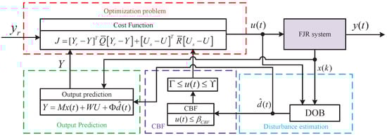
Figure 1. Control block Diagram of SDC-MPC.

To establish closed-loop stability and offset-free tracking, Equation (40) is equivalently written as:

$$\begin{array}{cc}\hfill \underset{u_0,\dots ,u_{N-1}}{min}& {∥x_N-{\overline{x}}_t∥}_F^2+\sum _{k=0}^{N-1}{∥x_k-{\overline{x}}_t∥}_Q^2+{∥u_k-{\overline{u}}_t∥}_R^2\hfill \\ \hfill \mathrm{s}.\mathrm{t}.& \Gamma \le u_k\le {\rm Y},k=0,1,\dots N\hfill \\ \hfill & x_{k+1}=A{x}_k+B{u}_k+B_d{d}_k\hfill \\ \hfill & d_{k+1}=d_k\hfill \\ \hfill & x_0=x\left(t\right)\hfill \\ \hfill & d_0=\widehat{d}\left(t\right)\hfill \end{array}$$

(41)

where $\Gamma =u_{min}$, ${\rm Y}=min\{u_{max},{\beta }_{CBF}\}$, and ${\overline{x}}_t,{\overline{u}}_t$ are the steady-state targets obtained from

$$\left[\begin{array}{cc}A-I& B\\ C& 0\end{array}\right]\left[\begin{array}{c}{\overline{x}}_t\\ {\overline{u}}_t\end{array}\right]=\left[\begin{array}{c}-B_d\widehat{d}\left(t\right)\\ y_r\end{array}\right].$$

(42)

Theorem 1.

Assuming that the MPC (41) is always feasible and the constraints are continuously satisfied, the steady-state error converges to zero, i.e., $y_{\infty }=y_r$.

Proof. 

First, according to Section 3.1, the prediction error satisfies

$$e_{ob}(t+1)={\Theta }_{ob}{e}_{ob}\left(t\right)$$

(43)

where ${\Theta }_{ob}=\left(L{B}_d-I\right)$ is Hurwitz under a suitable L.

As $t\to \infty$, the prediction model (32) yields

$$\left[\begin{array}{cc}A-I& B\\ C& 0\end{array}\right]\left[\begin{array}{c}{x}_{\infty }\\ u_{\infty }\end{array}\right]=\left[\begin{array}{c}-B_d{\widehat{d}}_{\infty }\\ y_{\infty }\end{array}\right].$$

(44)

Together with Equation (42), this implies

$$\left[\begin{array}{cc}A-I& B\\ C& 0\end{array}\right]\left[\begin{array}{c}\delta x_{\infty }\\ \delta u_{\infty }\end{array}\right]=\left[\begin{array}{c}0\\ y_{\infty }-y_r\end{array}\right]$$

(45)

where $\delta x_{\infty }=x_{\infty }-{\overline{x}}_{\infty }$ and $\delta u_{\infty }=u_{\infty }-{\overline{u}}_{\infty }$.

Define $\delta x_k=x_k-{\overline{x}}_t$ and $\delta u_k=u_k-{\overline{u}}_t$; then $y_k-y_r=C\delta x_k$. Problem (41) becomes

$$\begin{array}{cc}\hfill \underset{\delta u_0,\dots ,\delta u_{N-1}}{min}& {∥\delta x_N∥}_F^2+\sum _{k=0}^{N-1}{∥\delta x_k∥}_Q^2+{∥\delta u_k∥}_R^2\hfill \\ \hfill \mathrm{s}.\mathrm{t}.& \delta x_{k+1}=A\delta x_k+B\delta u_k,\delta x_0=x\left(t\right)-{\overline{x}}_t.\hfill \end{array}$$

(46)

Solving this problem yields $\delta u_0^{*}=k_{MPC}\delta x_0=u\left(t\right)-{\overline{u}}_t$, hence

$$u\left(t\right)=k_{MPC}\delta x_0+{\overline{u}}_t$$

(47)

with $k_{MPC}={(R+B^{T}FB)}^{-1}{B}^{T}FA$.

Letting $e_c\left(t\right)=x\left(t\right)-{\overline{x}}_t$, one obtains:

$$\begin{array}{cc}\hfill e_c(t+1)& =x(t+1)-{\overline{x}}_{t+1}\hfill \\ \hfill & =Ax\left(t\right)+Bu\left(t\right)+B_{d}d\left(t\right)-{\overline{x}}_{t+1}\hfill \\ \hfill & =(A+B{k}_{MPC})e_c\left(t\right)+B_d{e}_{ob}\left(t\right)\hfill \end{array}$$

(48)

where ${\Theta }_c=A+B{k}_{MPC}$ is Hurwitz. Therefore,

$$\left[\begin{array}{c}{e}_c(t+1)\\ e_{ob}(t+1)\end{array}\right]=\left[\begin{array}{cc}{\Theta }_c& B_d\\ 0& {\Theta }_{ob}\end{array}\right]\left[\begin{array}{c}{e}_c\left(t\right)\\ e_{ob}\left(t\right)\end{array}\right].$$

(49)

It follows that the closed-loop state matrix $\left[\begin{array}{cc}{\Theta }_c& B_d\\ 0& \Theta \end{array}\right]$ is Hurwitz, so $e_c\left(t\right)\to 0$. Since $y\left(t\right)-y_r=C(x\left(t\right)-{\overline{x}}_t)=C{e}_c\left(t\right)$, the tracking error converges to zero and thus $y_{\infty }=y_r$. □

4. Experimental Results

This section evaluates three controllers—traditional MPC, LQR + CBF, and the proposed SDC-MPC —in two scenarios: (i) persistent parametric uncertainty and (ii) external disturbances injected at a known time. Safety constraints are imposed on the joint angle; performance is assessed by angle-tracking accuracy, safety satisfaction, and angular-velocity smoothness.

The experimental platform parameters and nominal MPC weights are as stated previously (Figure 2). The control algorithms were implemented using MATLAB/Simulink (version 2022b, MathWorks, Natick, MA, USA). The relevant parameters of the experimental platform are $J_m=0.54\times {10}^{-3}\mathrm{kg}·{\mathrm{m}}^2$, $N_m=1$ and $K_m=38.5\mathrm{Nm}/\mathrm{rad}$, and the setup is shown in Figure 2. The controller parameters were rigorously tuned based on system dynamics and performance trade-offs. The prediction horizon was set to $N=10$ to balance the capability of capturing dominant transient dynamics (specifically flexible modes) against the computational load required for real-time execution. The weighting matrices were selected as $Q=10,000$ and $R=0.001$; this high $Q/R$ ratio prioritizes high-precision position tracking while permitting sufficient control authority to actively damp elastic oscillations within actuator limits. Finally, the DOB pole was placed at $p=-100$ following the bandwidth separation principle: this setting ensures the observer converges significantly faster than the outer motion control loop to effectively estimate time-varying disturbances, yet remains limited in bandwidth to prevent the amplification of high-frequency sensor noise. All quantitative results reported in this section represent the average performance metrics derived from three independent experimental trials to ensure statistical reliability.

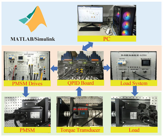
Figure 2. Experimental setup diagram.

4.1. Tests Under Persistent Parametric Uncertainty

Parametric uncertainty (e.g., inertia mismatch) is present throughout the tests. From a control viewpoint, such mismatch alters the effective inertia ratio and shifts the flexible mode, which tends to magnify boundary approaches when tracking near constraints. Controllers that do not tightly couple prediction, safety enforcement, and bias compensation are prone to either conservative tracking or boundary grazing.

Experiment 1 (angle constraint 0.5 rad). As a baseline, LQR designs a linear state-feedback for a linearized model and is paired with a CBF to enforce safety [12]. SDC-MPC achieves the smallest tracking error while strictly respecting the safety band. Quantitatively, Table 1 presents a comprehensive statistical analysis. In terms of safety, the maximum absolute error (MAE) is 0.051 rad for SDC-MPC, significantly lower than 0.151 rad for MPC and 0.300 rad for LQR + CBF. Moreover, SDC-MPC achieves the lowest root mean square error (RMSE) of 0.019 rad and integral absolute error (IAE) of 0.032 rad·s, indicating that it maintains the highest average tracking precision and minimal cumulative deviation throughout the task. The zoomed view shows visibly smaller excursions near the boundary for SDC-MPC, indicating tighter safety enforcement.

Table 1. Performance Statistics under Parametric Uncertainty (MAE: Max Absolute Error; MVF: Max Velocity Fluctuation).

Method	Tracking Error			MVF (rad/s)
	RMSE (rad)	MAE (rad)	IAE (rad·s)
MPC	0.055	0.151	0.118	14.019
LQR + CBF	0.112	0.300	0.245	21.177
SDC-MPC	0.019	0.051	0.032	8.732

The advantage comes from the way SDC-MPC embeds the CBF into the predictive optimization: the barrier constraint continuously re-shapes the admissible set so that candidate trajectories avoid unsafe neighborhoods, while the DOB reduces the effective model bias seen by the optimizer. As a result, the controller does not need to “fight” the mismatch with aggressive inputs; instead, it anticipates and moderates the motion, yielding both lower peak error and a clear safety margin in Figure 3.

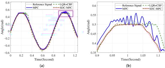
Figure 3. Parametric uncertainty, angle constraint $0.5\mathrm{rad}$. (a) Overall angle; (b) Zoomed angle.

With the 0.5 rad bound, SDC-MPC balances tracking and safety best, delivering the lowest peak error and the most conservative distance-to-boundary without sacrificing responsiveness.

Experiment 2 (angle constraint 0.45 rad). Under the tighter bound, SDC-MPC continues to enforce the constraint most effectively, with the smallest excursions near the limits and visibly faster recovery in the zoomed view.

Tight constraints accentuate the non-minimum-phase tendency of elastic joints: even modest overshoot can push the deflection towards the boundary. By coordinating prediction, barrier enforcement, and DOB compensation, SDC-MPC shapes the input to avoid exciting the flexible mode when close to the limit, hence the smaller excursions and faster re-convergence observed in Figure 4.

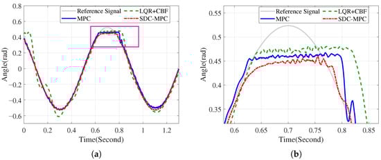
Figure 4. Parametric uncertainty, angle constraint $0.45\mathrm{rad}$. (a) Overall angle; (b) Zoomed angle.

With a 0.45 rad bound, SDC-MPC preserves a clear safety buffer and shortens the transient, maintaining constraint satisfaction despite the reduced feasible set.

Velocity responses (uncertainty). Across both constraints, SDC-MPC yields the smoothest dynamics and the lowest peak velocity, whereas LQR + CBF exhibits the largest fluctuations; MPC is intermediate.

Velocity smoothness reflects how effectively the controller damps the flexible mode while tracking. By compensating lumped bias via DOB and discouraging unsafe motions via CBF, the optimizer avoids high-gain “chasing” behavior, resulting in lower peaks and quicker decay in Figure 5.

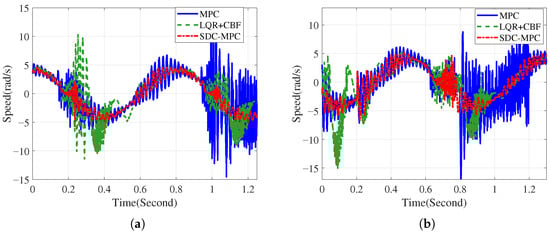
Figure 5. Angular-velocity responses under persistent parametric uncertainty. (a) With $0.5\mathrm{rad}$ constraint; (b) With $0.45\mathrm{rad}$ constraint.

SDC-MPC consistently reduces peak velocities and shortens damping time, indicating stronger elastic-mode suppression under persistent mismatch.

4.2. Tests Under External Disturbances (Injected at $t=$ 1.6 s)

Two groups are conducted with a disturbance injected at $t=1.6$ s (Figure 6). The focus is anti-disturbance capability while maintaining safety. The disturbance excites the flexible mode and challenges both compensation and constraint handling. To rigorously test robustness, a step torque disturbance with a magnitude of $6.66\mathrm{N}·\mathrm{m}$ was generated by the load motor and injected into the link side. This intentional perturbation emulates a sudden collision or payload change, creating a challenging scenario for stability and constraint enforcement.

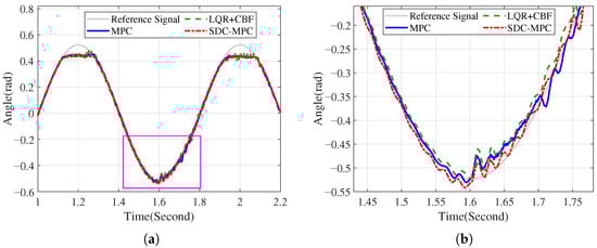
Figure 6. External disturbance (Group 1): angle tracking. (a) Overall; (b) Zoomed around $t=1.6$ s.

Group 1. SDC-MPC exhibits the smallest post-disturbance deviation and the fastest resettling in the angle response, while LQR + CBF shows the largest overshoot and oscillations; MPC is intermediate.

Immediately after the disturbance, uncompensated bias and aggressive recovery can amplify oscillations. SDC-MPC jointly limits unsafe excursions (CBF) and compensates the disturbance (DOB) within the horizon, steering the state back without boundary grazing. This explains the reduced peak and faster settling in the zoomed trajectory.

After $t=1.6$ s, SDC-MPC achieves the smallest angle excursion and quickest recovery while preserving the safety margin; MPC is moderate, and LQR + CBF is most sensitive.

Group 2. The same ordering holds: SDC-MPC achieves the smallest excursion immediately after the disturbance and the most rapid recovery; MPC is moderate; LQR + CBF is most sensitive.

Repeating the disturbance under a different operating instance confirms that the advantage is systematic rather than incidental. The combined DOB–CBF mechanism yields smaller peaks regardless of initial phasing, indicating robust rejection and constraint maintenance.

The second run reproduces the same ranking with lower peaks and faster decay for SDC-MPC, consolidating the anti-disturbance evidence.

Velocity responses under disturbances. Plotted together below, the two groups confirm that SDC-MPC suppresses speed spikes most effectively; MPC is moderate; LQR + CBF exhibits the largest peaks.

The peak speed after the disturbance is a sensitive indicator of rejection. By attenuating the lumped disturbance in prediction and constraining unsafe transients, SDC-MPC limits the initial spike and accelerates damping, consistent with the angle-domain findings.

In both groups, SDC-MPC yields the lowest peak speed and the fastest decay, showing the strongest suppression of disturbance-induced oscillations while preserving safety (Figure 7 and Figure 8).

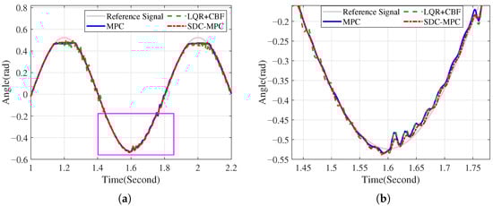
Figure 7. External disturbance (Group 2): angle tracking. (a) Overall; (b) Zoomed around $t=1.6$ s.

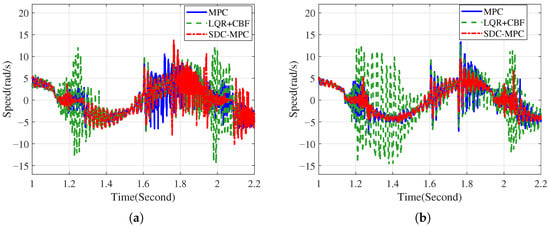
Figure 8. Angular-velocity under external disturbances (injected at $t=1.6$ s). (a) Group 1; (b) Group 2.

4.2.1. Quantitative Summary

Peak angle deviation and peak speed fluctuation near $t=1.6$ s are summarized in Table 2. Both groups show a consistent ranking, with SDC-MPC achieving the lowest peaks while ensuring constraint satisfaction. Additionally, the settling time (time to recover to steady state) is introduced to quantify rejection speed. As shown, SDC-MPC settles in approximately 0.15 s, less than half the time of MPC (0.32 s), demonstrating a decisive advantage in restoring equilibrium.

Table 2. Performance Statistics under External Disturbances (MAD: Max Angle Deviation; MSF: Max Speed Fluctuation; ST: Settling Time).

Metric	MPC	LQR + CBF	SDC-MPC
Group 1
MAD (rad)	0.165	0.300	0.055
MSF (rad/s)	13.5	19.5	8.5
ST (s)	0.32	0.55	0.15
Group 2
MAD (rad)	0.170	0.305	0.056
MSF (rad/s)	13.7	19.8	8.6
ST (s)	0.33	0.56	0.16

4.2.2. Real-Time Feasibility

To ensure the applicability of the proposed method in real-world scenarios, the computational load was logged during the experiments. The average computation time per MPC iteration was recorded at $6.66\mathrm{ms}$. This duration is well within the system’s sampling interval, confirming that the added complexity of the DOB and CBF constraints does not compromise the real-time performance of the SDC-MPC framework on the target hardware.

4.3. Parameter Sensitivity Analysis

To empirically validate the parameter selection discussed earlier, a sensitivity analysis was conducted regarding the prediction horizon N and the DOB bandwidth p. Table 3 summarizes the performance trade-offs based on the average of three experimental trials. It is observed that increasing N from 5 to 10 significantly reduces the tracking RMSE by capturing slower flexible modes, whereas further increasing N to 20 yields diminishing returns in accuracy but nearly doubles the computation time. Similarly, a moderate DOB pole ($p=-100$) provides the best balance between disturbance rejection (low MAE) and noise amplification (low velocity fluctuation), validating the chosen tuning.

Table 3. Sensitivity Analysis of Controller Parameters (Average of 3 Trials).

Parameter Setting	RMSE (rad)	MVF (rad/s)	Comp. Time (ms)
Impact of Prediction Horizon (N)
$N=5$ (Short)	0.035	9.2	3.1
$N=10$ (Nominal)	0.019	8.7	6.7
$N=20$ (Long)	0.018	8.6	14.2
Impact of DOB Pole (p)
$p=-50$ (Slow)	0.028	5.1	6.7
$p=-100$ (Nominal)	0.019	8.7	6.7
$p=-200$ (Fast)	0.017	15.3	6.7

In summary, the experiments demonstrate that the proposed SDC-MPC consistently strengthens safety-constraint satisfaction and robust tracking under both persistent parametric uncertainty and injected external disturbances. Compared with the baselines (MPC and LQR + CBF), it exhibits smaller boundary excursions, smoother velocity transients, and faster recovery without compromising stability, highlighting its suitability for flexible-joint robots operating in interaction-rich, safety-critical scenarios.

5. Discussion

The experimental results presented in Section 4 demonstrate that the proposed SDC-MPC framework significantly outperforms standard MPC and baseline safety schemes in terms of tracking accuracy, disturbance rejection, and constraint satisfaction. This section analyzes the underlying mechanisms driving these improvements, compares the findings with existing literature, and critically discusses the limitations of the current study.

5.1. Comparative Analysis with Recent Frameworks

To explicitly position the proposed method within the recent literature, Table 4 summarizes the key structural differences between SDC-MPC and existing decoupled architectures. We evaluate four critical architectural attributes: disturbance compensation (DC), which indicates the presence of an active observer; formal safety (FS), denoting the use of control barrier functions; disturbance-aware safety (DAS), representing the adaptive coupling between estimation and constraints; and feasibility assurance (FA), referring to mechanisms that prevent solver failure. While recent DOB-based approaches [19,20] focus on DC and CBF-based methods [25,26] prioritize FS, they typically treat these objectives in isolation (DAS: No). The proposed SDC-MPC distinguishes itself by introducing a DAS mechanism, where the estimated disturbance directly modulates the CBF constraints. This unique coupling allows the system to maintain strict safety under varying loads without the excessive conservatism found in robust MPC or the feasibility issues common in hard-constrained schemes.

Table 4. Comparison of Control Frameworks for FJRs (DC: Disturbance Compensation; FS: Formal Safety; DAS: Disturbance-Aware Safety; FA: Feasibility Assurance).

Framework	DC	FS	DAS	FA
MPC + DOB [19,20]	Yes	No	No	Hard
MPC + CBF [25,26]	No	Yes	No	Filter-Dep.
Robust MPC	Worst-Case	Yes	Fixed	Conservative
SDC-MPC (Ours)	Yes	Yes	Yes	Soft

5.2. Mechanism of Performance Enhancement

The superior performance of SDC-MPC can be attributed to the tight coupling between disturbance estimation and safety enforcement. In conventional decoupled approaches (e.g., MPC + DOB without disturbance-aware safety, or MPC+CBF without disturbance compensation), a conflict often arises: the DOB attempts to cancel external forces by demanding aggressive torques, which may drive the system towards state limits, subsequently triggering the safety filter to abruptly cut off inputs. This “fighting” effect leads to the oscillations observed in the LQR + CBF baseline.

In contrast, SDC-MPC integrates the estimated disturbance $\widehat{d}$ directly into the predictive model used by the CBF mechanism (via the ${\beta }_{CBF}$ constraint). This allows the controller to anticipate the trajectory deviation caused by the load and the necessary safety margin adjustment simultaneously. Consequently, the solver finds an optimal path that compensates for the disturbance within the safe set, rather than reacting to safety violations after they occur. This structural advantage explains the reduced settling time and lower MAE observed in Table 2.

5.3. Limitations and Future Work

While the proposed method shows promise, several limitations inherent to the current study must be acknowledged to provide a balanced perspective for future research.

5.3.1. Scalability to Multi-Joint Systems

The current validation is conducted on a single-link flexible-joint manipulator. While this setup effectively isolates the fundamental challenges of elasticity and motor-link coupling, extending the method to multi-degree-of-freedom (multi-DOF) robots introduces complex nonlinearities, such as Coriolis and centrifugal forces, which are coupled across joints. Although the theoretical formulation of DOB and CBF can be extended to multi-variable systems, the computational load for the MPC solver will increase quadratically. Future work will investigate efficient solvers (e.g., explicit MPC or warm-started SQP) to maintain real-time feasibility for multi-joint platforms.

5.3.2. Modeling Simplifications

The dynamic model derived in Section 2 assumes linear joint elasticity and ignores nonlinear friction phenomena (e.g., the Stribeck effect) or hysteresis in the harmonic drive. In practice, gear transmission often exhibits nonlinear stiffness and backlash. Although the DOB effectively lumps these unmodeled dynamics into the disturbance term $d_1$, relying entirely on the observer for significant structural nonlinearities may degrade the prediction horizon’s accuracy. Integrating data-driven friction models or nonlinear stiffness curves into the prediction model could further enhance performance.

5.3.3. Noise Sensitivity and Bandwidth Trade-Off

The efficacy of SDC-MPC relies heavily on the quality of the disturbance estimate. As noted in the parameter tuning, a high-bandwidth DOB ($p=-100$) allows for fast disturbance tracking but risks amplifying measurement noise. In the experiments, high-precision encoders were used; however, in industrial settings with lower-resolution sensors or significant electromagnetic interference, the noise amplified by the differentiation in the observer could lead to chattering in the control input. This necessitates a careful trade-off between disturbance rejection speed and noise robustness, or the adoption of advanced filtering techniques (e.g., Kalman Filter-based DOB) in noise-prone environments.

6. Conclusions

This paper addressed the conflict between high-precision tracking and strict safety enforcement in flexible-joint robots (FJRs) by proposing the SDC-MPC framework, which unifies disturbance observation and control barrier functions within predictive optimization. Comprehensive experiments on a hardware platform demonstrated that the proposed method significantly enhances robustness and safety compared to decoupled architectures. Quantitatively, SDC-MPC reduced tracking RMSE by over 65% compared to standard MPC and halved the settling time under external shock loads to approximately 0.15 s, all while rigorously maintaining safety constraints during fast transients. Practically, these results imply that FJRs can operate closer to their physical limits with higher reliability, which is critical for efficiency in collaborative manufacturing and interaction-rich scenarios.

Despite these advancements, the current study is limited to a single-joint configuration with linearized elasticity assumptions, which may not fully capture the complex multi-body couplings and nonlinear transmission effects (e.g., hysteresis) present in full-scale manipulators. Consequently, future research will focus on three key directions: (1) extending the framework to multi-degree-of-freedom systems with coupled nonlinear dynamics; (2) incorporating data-driven friction and stiffness models to further reduce prediction bias; and (3) investigating efficient numerical solvers, such as explicit MPC or warm-started SQP, to ensure real-time feasibility as the system dimension increases.

References

- Albu-Schffer, A.; Ott, C.; Hirzinger, G. A Unified Passivity-Based Control Framework for Position, Torque and Impedance Control of Flexible Joint Robots. Int. J. Robot. Res. 2007, 26, 23–39. [Google Scholar] [CrossRef]
- Ott, C.; Albu-Schffer, A.; Kugi, A.; Hirzinger, G. On the Passivity-Based Impedance Control of Flexible Joint Robots. IEEE Trans. Robot. 2008, 24, 416–429. [Google Scholar] [CrossRef]
- Mansfeld, N.; Keppler, M.; Haddadin, S. Speed Gain in Elastic Joint Robots: An Energy Conversion-Based Approach. IEEE Robot. Autom. Lett. 2021, 6, 4600–4607. [Google Scholar] [CrossRef]
- Spyrakos, P.E.; Dai, J.S. Stable Flexible-Joint Floating-Base Robot Balancing and Locomotion via Variable Impedance Control. IEEE Trans. Ind. Electron. 2023, 70, 2748–2758. [Google Scholar] [CrossRef]
- Jin, M.; Lee, J.; Tsagarakis, N.G. Model-Free Robust Adaptive Control of Humanoid Robots With Flexible Joints. IEEE Trans. Ind. Electron. 2017, 64, 1706–1715. [Google Scholar] [CrossRef]
- Zhihua, Q. Input-output robust tracking control design for flexible joint robots. IEEE Trans. Autom. Control 1995, 40, 78–83. [Google Scholar] [CrossRef]
- An-Chyau, H.; Yuan-Chih, C. Adaptive sliding control for single-link flexible-joint robot with mismatched uncertainties. IEEE Trans. Control Syst. Technol. 2004, 12, 770–775. [Google Scholar]
- Rsetam, K.; Cao, Z.; Man, Z. Design of Robust Terminal Sliding Mode Control for Underactuated Flexible Joint Robot. IEEE Trans. Syst. Man Cybern. Syst. 2022, 52, 4272–4285. [Google Scholar] [CrossRef]
- Spong, M.W. Adaptive Control of Flexible Joint Manipulators: Comments on Two Papers. Automatica 1995, 31, 585–590. [Google Scholar] [CrossRef]
- Jiang, H.; Yang, Y.; Hua, C.; Li, X.; Lu, F. Predefined-Time Composite Fuzzy Adaptive Control for Flexible-Joint Manipulator System With High-Order Fully Actuated Control Approach. IEEE Trans. Ind. Electron. 2025, 72, 7191–7199. [Google Scholar] [CrossRef]
- Yang, K.; Zhao, L. Command-Filtered Backstepping Control for Flexible Joint Manipulator Systems with Full-State Constraints. Int. J. Control Autom. Syst. 2022, 20, 2231–2238. [Google Scholar] [CrossRef]
- Doina, Z.M. LQG/LQR optimal control for flexible joint manipulator. In Proceedings of the 2012 International Conference and Exposition on Electrical and Power Engineering, Iasi, Romania, 25–27 October 2012; pp. 35–40. [Google Scholar]
- Maeder, U.; Borrelli, F.; Morari, M. Linear offset-free Model Predictive Control. Automatica 2009, 45, 2214–2222. [Google Scholar] [CrossRef]
- Hasan, M.N.; Haris, M.; Pirzada, S.J.H.; Qin, S. Adaptive Model Predictive Control for a Class of Nonlinear Single-Link Flexible Joint Manipulator. In Proceedings of the 2019 Second International Conference on Latest Trends in Electrical Engineering and Computing Technologies (INTELLECT), Karachi, Pakistan, 13–14 November 2019; pp. 1–6. [Google Scholar]
- Sun, J.; Peng, C.; Zou, J.; Zhou, Q.; Wu, Y. A novel MPC-NNSMC composite control method for robotic manipulators considering uncertainties and constraints. Control Eng. Pract. 2025, 156, 106238. [Google Scholar] [CrossRef]
- Pradhan, S.K.; Subudhi, B. Nonlinear Adaptive Model Predictive Controller for a Flexible Manipulator: An Experimental Study. IEEE Trans. Control Syst. Technol. 2014, 22, 1754–1768. [Google Scholar] [CrossRef]
- Mayne, D.Q.; Rawlings, J.B.; Rao, C.V.; Scokaert, P.O.M. Constrained Model Predictive Control: Stability and Optimality. Automatica 2000, 36, 789–814. [Google Scholar] [CrossRef]
- Kim, M.J.; Chung, W.K. Disturbance-Observer-Based PD Control of Flexible Joint Robots for Asymptotic Convergence. IEEE Trans. Robot. 2015, 31, 1508–1516. [Google Scholar] [CrossRef]
- Tian, L.; Gao, Y.; Zhang, Z. Disturbance-observer-based tracking controller for a flexible-joint robotic manipulator with full-state constraints. Proc. Inst. Mech. Eng. Part I J. Syst. Control Eng. 2022, 236, 1166–1175. [Google Scholar] [CrossRef]
- Lee, D.; Back, J.; Oh, S. Workspace Nonlinear Disturbance Observer for Robust Position Control of Flexible Joint Robots. IEEE Robot. Autom. Lett. 2024, 9, 4495–4502. [Google Scholar] [CrossRef]
- Yang, J.; Zheng, W.X.; Li, S.; Wu, B.; Cheng, M. Design of a Prediction-Accuracy-Enhanced Continuous-Time MPC for Disturbed Systems via a Disturbance Observer. IEEE Trans. Ind. Electron. 2015, 62, 5807–5816. [Google Scholar] [CrossRef]
- Yan, Y.; Yang, J.; Sun, Z.; Li, S.; Yu, H. Non-linear-disturbance-observer-enhanced MPC for motion control systems with multiple disturbances. IET Control Theory Appl. 2020, 14, 63–72. [Google Scholar] [CrossRef]
- Ames, A.D.; Coogan, S.; Egerstedt, M.; Notomista, G.; Sreenath, K.; Tabuada, P. Control Barrier Functions: Theory and Applications. In Proceedings of the 2019 18th European Control Conference (ECC), Naples, Italy, 25–28 June 2019. [Google Scholar]
- Kurtz, V.; Wensing, P.M.; Lin, H. Control Barrier Functions for Singularity Avoidance in Passivity-Based Manipulator Control. In Proceedings of the 2021 60th IEEE Conference on Decision and Control (CDC), Austin, TX, USA, 14–17 December 2021; pp. 6125–6130. [Google Scholar]
- Heshmati-Alamdari, S.; Sharifi, M.; Karras, G.C.; Fourlas, G.K. Control barrier function based visual servoing for Mobile Manipulator Systems under functional limitations. Robot. Auton. Syst. 2024, 182, 104813. [Google Scholar] [CrossRef]
- Liu, J.; Yang, J.; Mao, J.; Zhu, T.; Xie, Q.; Li, Y.; Wang, X.; Li, S. Flexible Active Safety Motion Control for Robotic Obstacle Avoidance: A CBF-Guided MPC Approach. IEEE Robot. Autom. Lett. 2025, 10, 2686–2693. [Google Scholar] [CrossRef]
- Ott, C.; Roa, M.A.; Albu-Schäffer, A. An Experimental Study on MPC-Based Joint Torque Control for Flexible Joint Robots. IEEE Robot. Autom. Lett. 2019, 4, 4201–4208. [Google Scholar] [CrossRef]
- Chen, W.H.; Yang, J.; Guo, L.; Li, S. A general nonlinear MPC framework for disturbances rejection. In Proceedings of the 19th World Congress the International Federation of Automatic Control, Cape Town, South Africa, 24–29 August 2014; Volume 47, pp. 4640–4645. [Google Scholar]
- Zeng, J.; Zhang, B.; Sreenath, K. Safety-Critical Model Predictive Control with Discrete-Time Control Barrier Functions. In Proceedings of the 2021 American Control Conference (ACC), New Orleans, LA, USA, 25–28 May 2021; pp. 3882–3889. [Google Scholar]
- Singletary, A.; Ames, A.D. Comparative Analysis of Control Barrier Functions and Artificial Potential Fields for Obstacle Avoidance. In Proceedings of the 2021 IEEE/RSJ International Conference on Intelligent Robots and Systems (IROS), Prague, Czech Republic, 27 September–1 October 2021; pp. 8129–8136. [Google Scholar]
Disclaimer/Publisher’s Note: The statements, opinions and data contained in all publications are solely those of the individual author(s) and contributor(s) and not of MDPI and/or the editor(s). MDPI and/or the editor(s) disclaim responsibility for any injury to people or property resulting from any ideas, methods, instructions or products referred to in the content. |
© 2025 by the authors. Licensee MDPI, Basel, Switzerland. This article is an open access article distributed under the terms and conditions of the Creative Commons Attribution (CC BY) license (https://creativecommons.org/licenses/by/4.0/).