Distributed State Estimation for Bilinear Power System Models Based on Weighted Least Absolute Value

Abstract

Accurate, scalable, and outlier-robust state estimation (SE) is critical for large AC power systems with mixed SCADA and PMU measurements. This paper proposes D-BSE-L1, a distributed robust state estimator for the bilinear AC model. The method combines the bilinear state estimation framework with a convex weighted least absolute value (WLAV) loss so that all area subproblems become convex linear or quadratic programs coordinated by ADMM, and a cache-enabled Cholesky factorization is used to accelerate the third-stage linear solves. Simulations on the IEEE 14-, 118-, and 1062-bus systems show that D-BSE-L1 achieves estimation accuracy comparable to its centralized bilinear counterpart. Under severe bad-data conditions, its advantage over weighted least squares with the largest normalized residual test (WLS + LNRT) is pronounced: with 10% 1.5× bad data, the voltage magnitude and angle MAEs are about 62% and 54% of those of WLS + LNRT, and with 5% 5× bad data, they further drop to roughly 43% and 51%, while requiring only about one-tenth of the CPU time. On the 1062-bus system, D-BSE-L1 maintains the MAE of the centralized estimator but reduces runtime from 2.46 s to 0.72 s, providing a scalable, hyperparameter-free, and robust solution for partitioned state estimation in large-scale power grids.

1. Introduction

Recent energy transitions and the evolving modes of power system operation have imposed stricter requirements on grid dispatch, security, and stability. The large-scale integration of variable renewable generation, together with the rapid proliferation of distributed energy resources and flexible loads, has rendered grid operations increasingly uncertain, expanded network scale, and introduced measurement data with non-Gaussian noise characteristics [1,2]. Against this backdrop, power system state estimation (PSSE)—a core function of modern energy management systems—must efficiently, robustly, and scalably convert raw measurements into reliable estimates of bus voltage magnitudes and phase angles in the presence of complex noise and anomalous observations, thereby supplying trustworthy inputs to downstream applications such as stability assessment, optimal power flow, and economic dispatch [3].

Since the 1970s, weighted least squares (WLS) has been the de facto standard for PSSE [4,5]. However, WLS relies on linearization of the measurement model and Gauss–Newton iterations, so Jacobian construction and normal-equation factorization incur high computational and memory costs in large-scale networks; moreover, its quadratic loss formulation is sensitive to bad data and heavy-tailed noise. With the fusion of phasor measurement unit (PMU) and supervisory control and data acquisition (SCADA) data and increasingly complex communication infrastructures, anomalous measurements have become more frequent, and WLS alone is insufficient to meet both real-time and robustness requirements, thereby motivating the development of robust state estimation frameworks that are scalable, amenable to large-scale parallel computing, and tailored to non-Gaussian noise environments [6].

Centralized state estimation aggregates system-wide measurements at a single control center, rendering it vulnerable to computational bottlenecks, heavy communication burdens, single points of failure, and data privacy risks. By contrast, distributed state estimation divides the power system into multiple areas and requires exchanging only a small number of boundary consensus variables; each area independently solves its local subproblem while coordinating to achieve global consistency. This architecture enhances scalability, robustness, and reliability while preserving estimation consistency across the network. It aligns naturally with distributed optimization frameworks—most notably alternating direction method of multipliers (ADMM)—and offers a practical pathway to real-time state estimation in large-scale systems [7].

Distributed and decentralized state estimation has been extensively explored along several methodological lines. Xie et al. proposed a modified coordinated state estimation scheme in which each control area initializes a full-system state vector and exchanges boundary information with predefined neighbors; under this protocol, the local estimates converge to the centralized solution [8]. Minot et al. employed matrix-splitting techniques to compute the Gauss–Newton search direction in a distributed fashion, reporting substantially faster convergence than distributed gradient methods [9]. Building on quasi-Newton ideas, Zheng et al. developed an adaptive distributed BFGS-type algorithm with superlinear local convergence and an adaptive step-size rule that mitigates the slow convergence or divergence caused by improper step sizes [10]. Cosović et al. integrated belief propagation into the Gauss–Newton framework and reported accuracy comparable to the centralized estimator; relative to matrix-splitting approaches, their method exhibited improved robustness to ill-conditioning induced by numerous pseudo-measurements [11]. On an overlapping sub-area decomposition, Kekatos et al. formulated a distributed linear state estimator with bad-data resilience, proved its equivalence to Huber’s M-estimator in the centralized case, and solved it via ADMM [12]. Finally, Zou et al. solved the primal nonlinear model using ADMM and introduced dynamic tuning of the quadratic penalty parameter; their experiments indicated that the penalty can be selected without prior tuning knowledge [13].

While the aforementioned studies have realized distributed state estimation for power systems utilizing various distributed optimization strategies, the majority rely on WLS and fail to incorporate robust estimation techniques. Consequently, the reliability of these estimators is compromised in the presence of bad data and non-Gaussian noise. To improve robustness, C. H. Ho et al. adopted Hampel’s three-part redescending ψ-function to attenuate bad-data effects and further proposed a robust weight-smoothing mechanism that accelerates and stabilizes convergence, with performance reported to outperform L1-ADMM under outlier contamination [14]. Chen et al. developed a distributed robust estimator based on the maximum correntropy criterion (MCC) coupled with a finite-time average-consensus protocol; their method demonstrated strong estimation accuracy under non-Gaussian noise and resilience to intermittent communication failures [15]. In a related line, Chen et al. also introduced a generalized loss that remains quadratic for small residuals but switches—through shape and scale parameters—to a heavier-tailed form for large residuals; distributed computation is effected via matrix splitting, and experiments indicate stronger robustness to non-Gaussian noise than the Huber loss [16]. Lin et al. extended the bad-data-aware linear model of [12] to active distribution networks, relaxing the L1 term and recasting the problem as a quadratic program (QP). With a distributed coordination mechanism, each iteration exchanges only quadratic functions of boundary-state variables [17]. Finally, Zhang et al. formulated a relative-error-based robust estimator that avoids the instability arising from a uniform absolute tolerance across measurements with heterogeneous magnitudes. Suspicious data are pre-screened via projection statistics and a normalized residual test, and the optimization is solved by an embedded-consensus ADMM using an outer-approximation scheme [18].

The aforementioned studies achieve robust state estimation by evaluating the performance of robust loss functions in power system state estimation or by formulating mathematical models that incorporate bad data. However, these methods typically necessitate specific hyperparameter settings that necessitate a trade-off between statistical efficiency and robustness. Consequently, their performance may be suboptimal in the presence of unknown non-ideal measurements. Furthermore, refs. [15,16] employ non-convex loss functions, for which the global optimality of the estimation results cannot be mathematically guaranteed.

Bilinear state estimation (BSE) for power systems transforms the original nonlinear, non-convex optimization model into two linear convex optimization models coupled with a nonlinear transformation process. This approach facilitates the resolution of global optimality and convergence issues in power system state estimation while preserving physical consistency [19,20,21].

Building upon the BSE framework, this paper implements distributed state estimation by replacing the WLS estimator with the WLAV estimator and integrating ADMM. The proposed method eliminates the need for hyperparameter tuning of the robust loss function and provides a mathematical guarantee for the global optimality of the solution. Furthermore, by leveraging the high-precision phase angle measurements provided by PMUs, the proposed method further enhances the estimation accuracy of the linear model in the third stage of BSE. The main contributions are as follows:

(1)

Distributed robust framework for the bilinear model. This paper establishes a WLAV-based framework that combines the bilinear measurement model with an ADMM coordination mechanism, enabling distributed power system state estimation that jointly emphasizes robustness and computational speed.

(2)

Solution scheme for the L1 loss. Under the WLAV criterion, we present the mathematical derivation of the first-stage state vector update. By introducing auxiliary variables and applying variable relaxation, the non-differentiable L1 objective is transformed into a convex QP, thereby ensuring accurate and efficient sub-area state updates.

(3)

Computational acceleration. In the third stage of the algorithm, the local state update requires solving a symmetric positive-definite linear system. We apply Cholesky factorization to decompose the system into two triangular solves via forward–backward substitution, reducing the overall computational cost.

The remainder of this paper is organized as follows: Section 2 reviews the traditional nonlinear power system state estimation based on the WLS method and its distributed form. Section 3 introduces BSE and proposes its distributed state estimation form. Section 4, based on the L1 loss function, proposes the distributed robust state estimation method based on the bilinear model and presents a computational acceleration method. Section 5 presents the simulation results and analyzes the performance of the proposed algorithm. Section 6 provides the conclusion of this paper.

2. Nonlinear Distributed PSSE Model

2.1. Distributed State Estimation Model

This section first reviews the mathematical formulation of the conventional centralized power system SE problem and, building on it, constructs a generic distributed SE model. The latter partitions the network into multiple sub-areas and introduces consensus constraints on shared boundary states, thereby laying the groundwork for the distributed optimization algorithms developed later. As illustrated in Figure 1, for two adjacent sub-areas, the boundary buses—1 through 4—and their incident tie-lines are represented in both Area 1 and Area 2. The overlap therefore includes the state variables and associated measurements of buses 1–4, as well as the measurements on tie-lines (1–2) and (3–4).

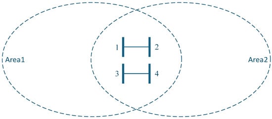
Figure 1. Overlapping partition of Area 1 and Area 2. (Numbers 1–4 denote the power system nodes located in the overlapping region between Areas 1 and 2.).

In centralized state estimation, the power system measurement equations can be modeled as the following nonlinear measurement equations:

$$z=h(x)+e$$

(1)

where $z\in R^m$ is the measurement vector, $x\in R^n$ is the state vector, $h\left(x\right):R^n\to R^m$ is a nonlinear differentiable function relating the state vector to the measurements, and $e$ is the measurement error vector, which follows a Gaussian distribution with a mean of 0 and a standard deviation of $\sigma$, denoted as $e~N\left(0,{\sigma }^2\right)$.

To address the scalability challenges of large-scale power grids, we extend this model to a distributed framework. The distributed state estimator for the power system is illustrated in Figure 2. For a power system comprising $k$ sub-areas, its measurement equations can be expressed as:

$$z_k=h_k\left(x_k\right)+e_k$$

(2)

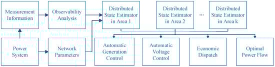
Figure 2. Distributed state estimator for power systems.

According to WLS, the state estimation objective function for each sub-area is:

$$\min J_k\left(x_k\right)={\left[z_k-h_k\left(x_k\right)\right]}^{{\rm T}}{R}_k^{-1}\left[z_k-h_k\left(x_k\right)\right]$$

(3)

The overall objective function for distributed state estimation is expressed as follows:

$$\begin{array}{c}\min {\displaystyle \sum _{k=1}^K{J}_k\left(x_k\right)}\\ s.t.x_k\left[l\right]=x_l\left[k\right],\forall l\in N_k,\forall k\end{array}$$

(4)

where $N_k$ denotes the set of areas that share states with area $k$. For any two adjacent areas $k$ and $l$, $x_k\left[l\right]$ represents the state vector in area $k$ that overlaps with area $l$. The equality constraints ensure the consistency of shared state variables between adjacent areas. To implement the distributed algorithm, an auxiliary variable $x_{kl}$ is introduced for the shared state variables of each adjacent area, i.e., $x_{kl}=x_k\left[l\right]=x_l\left[k\right]=x_{lk}$. The new equality constraints can be written as:

$$x_{kl}=x_k\left[l\right],\forall l\in N_k,\forall k$$

(5)

2.2. Distributed State Estimation Based on ADMM

Distributed state estimation in power systems constitutes a distributed consensus optimization problem. To solve this problem efficiently, this paper employs ADMM. This approach decomposes the original problem into multiple subproblems that can be solved in parallel and utilizes the method of multipliers to coordinate their solutions, thereby providing a distributed algorithm that efficiently solves large-scale optimization problems. ADMM has been extensively studied for its application in power system distributed state estimation [22,23]. Using the method of Lagrangian multipliers, the optimization model for distributed state estimation is transformed into the following form:

$$L\left(\left\{x_k\right\},\left\{x_{kl}\right\};\left\{v_{k,l}\right\}\right)={\displaystyle \sum _{k=1}^K\left[J_k(x_k)+{\displaystyle \sum _{l\in N_k}\left(v_{k,l}^{{\rm T}}(x_k\left[l\right]-x_{kl})+\frac{\rho }{2}{‖x_k\left[l\right]-x_{kl}‖}_2^2\right)}\right]}$$

(6)

where $v_{k,l}$ is the Lagrangian multiplier, and $\rho$ is the penalty parameter of ADMM, with $\rho >0$. This parameter is introduced to penalize solutions that do not satisfy the consistency constraints, and its value has a significant impact on the algorithm’s convergence speed. The ADMM algorithm, by decomposing the original problem into multiple subproblems and solving them through alternating iterations, is inherently suited for the requirements of distributed computation. The ADMM algorithm iterates through the following three steps:

$$\{x_k^{t+1}\}:=\arg \underset{x_k}{\min }L(\{x_k^t\},\{x_{kl}^t\};\{v_{k,l}^t\})$$

(7)

$$\{x_{kl}^{t+1}\}:=\arg \underset{x_{kl}}{\min }L(\{x_k^{t+1}\},\{x_{kl}^t\};\{v_{k,l}^t\})$$

(8)

$$v_{k,l}^{t+1}:=v_{k,l}^t+\rho (x_k^{t+1}[l]-x_{kl}^{t+1}),\forall k,\forall l$$

(9)

According to [12], Equations (7)–(9) are equivalent to the following form:

$$x_k^{t+1}:=\arg \underset{x_k}{\min }\left\{J_k(x_k)+{\displaystyle \frac{\rho }{2}}{\displaystyle \sum _{\underset{N_k^i\ne \varnothing }{i=1}}^{N_k}\left|N_k^i\right|}{\left(x_k(i)-p_k^t(i)\right)}^2\right\},\forall k$$

(10)

$$s_k^{t+1}:={\displaystyle \frac{1}{\left|N_k^i\right|}}{\displaystyle \sum _{l\in N_k^i}{x}_l^{t+1}\left[i\right]},\forall i with N_k^i\ne \varnothing$$

(11)

$$p_k^{t+1}(i):=p_k^t(i)+s_k^{t+1}(i)-{\displaystyle \frac{x_k^t(i)+s_k^t(i)}{2}}, \forall i, N_k^i\ne \varnothing$$

(12)

Equations (10)–(12) constitute the distributed iterative solution framework for power systems based on the ADMM algorithm. Within this framework, Equations (10) and (12) can be updated at the respective sub-area power system control centers. The averaging step in Equation (11) can be completed either by a coordinator or locally.

3. Distributed BSE

3.1. Distributed BSE Model

In PSSE, the measurement vector typically includes the voltage magnitude $V_i$ at bus $i$, the bus power injections $P_i$ and $Q_i$, and the branch power flows $P_{ij}$ and $Q_{ij}$. Their exact mathematical expressions are as follows:

$$P_i=V_i{\displaystyle \sum }_{j\in i}{V}_j\left(G_{ij}\cos {\theta }_{ij}+B_{ij}\sin {\theta }_{ij}\right)$$

(13)

$$Q_i=V_i{\displaystyle \sum }_{j\in i}{V}_j\left(G_{ij}\sin {\theta }_{ij}-B_{ij}\cos {\theta }_{ij}\right)$$

(14)

$$P_{ij}=v_i^2\left(g_{si}+g_{ij}\right)-v_i{v}_j{g}_{ij}\cos {\theta }_{ij}-v_i{v}_j{b}_{ij}\sin {\theta }_{ij}$$

(15)

$$Q_{ij}=-v_i^2\left(b_{\mathrm{s}i}+b_{ij}\right)+v_i{v}_j{b}_{ij}\cos {\theta }_{ij}-v_i{v}_j{g}_{ij}\sin {\theta }_{ij}$$

(16)

where ${\theta }_{ij}={\theta }_i-{\theta }_j$. From the mathematical expressions of the measurement Equations (13)–(16), it is evident that the original power system measurement equation $z=h\left(x\right)$ is a nonlinear and non-convex function. Bilinear state estimation, however, employs variable substitution to transform the original problem into two linear estimation stages and one nonlinear transformation stage, thereby simplifying the computation.

Let $U_i=V_i^2$, $K_{ij}=V_i{V}_{j}cos{ \theta }_{ij}$ and $L_{ij}=V_i{V}_{j}sin{ \theta }_{ij}$. Then the state vector for the first-stage linear model is $y=\left\{U_i, K_{ij}, L_{ij}\right\}$. The measurement vector $\tilde{z}$ is $\tilde{z}=\left\{U_i, P_i,Q_i, P_{ij},Q_{ij}\right\}$. The new measurement equations can be expressed as:

$$\tilde{z}=By+e_z$$

(17)

The new linear matrix $B$ is a coefficient matrix, and its exact mathematical expression is as follows:

$$B=\left[\begin{array}{ccc}1& 0& 0\\ G_{ii}& G_{ij}& B_{ij}\\ -B_{ii}& -B_{ij}& G_{ij}\\ g_{si}+g_{ij}& -g_{ij}& -b_{ij}\\ -(b_{si}+b_{ij})& b_{ij}& -g_{ij}\\ {\alpha }_{U_i}& {\alpha }_K& {\alpha }_L\end{array}\right]$$

(18)

where ${\alpha }_{U_i}=g_{ij}^2+{\left(b_{ij}+b_{si}\right)}^2$, ${\alpha }_K=-2\left(g_{ij}^2+b_{ij}^2+b_{ij}{b}_{si}\right)$ and ${\alpha }_L=2g_{ij}{b}_{si}$. The distributed state estimation model for the first stage can be written as:

$$\begin{array}{c}\min {\displaystyle \sum _{k=1}^K{\left[{\tilde{z}}_k-B_k{y}_k\right]}^{{\rm T}}{W}_{yk}}\left[{\tilde{z}}_k-B_k{y}_k\right]\\ s.t.y_k\left[l\right]=y_{kl},\forall l\in N_k,\forall k\end{array}$$

(19)

where $W_{yk}$ is the weight matrix for each area $k$. For ease of notation, we define a diagonal matrix $D_k$ for each area $k$, whose $\left(i,i\right)$-th element is $\left|N_k^i\right|$. By applying the ADMM distributed framework described in Section 2 to this linearized model, the optimization objective function framework for the first stage of distributed bilinear state estimation can be obtained as:

$$\begin{array}{c}{y}_k^{t+1}=\arg \underset{y_k}{\min }\left\{{\displaystyle \sum _{k=1}^K{\left[{\tilde{z}}_k-B_k{y}_k\right]}^{{\rm T}}{W}_{yk}}\left[{\tilde{z}}_k-B_k{y}_k\right]+{\displaystyle \frac{\rho }{2}}{\displaystyle \sum _{\underset{N_k^i\ne \varnothing }{i=1}}^{N_k}\left|N_k^i\right|}{\left(y_k(i)-p_k^t(i)\right)}^2\right\}\\ ={\left(B_k^{{\rm T}}{W}_{yk}{B}_k+\rho D_k\right)}^{-1}\left(B_k^{{\rm T}}{W}_{yk}{\tilde{z}}_k+\rho D_k{p}_k\right)\end{array}$$

(20)

$$s_k^{t+1}={\displaystyle \frac{1}{\left|N_k^i\right|}}{\displaystyle \sum _{l\in N_k^i}{y}_l^{t+1}\left[i\right]}$$

(21)

$$p_k^{t+1}(i)=p_k^t(i)+s_k^{t+1}(i)-{\displaystyle \frac{y_k^t(i)+s_k^t(i)}{2}}$$

(22)

In the second stage, the state vector from the first stage undergoes the following nonlinear transformation:

$$a_i=\ln U_i=2\ln V_i$$

(23)

$$a_{ij}=\ln \left(K_{ij}^2+L_{ij}^2\right)=a_i+a_j$$

(24)

$${\theta }_{ij}=\arctan {\displaystyle \frac{L_{ij}}{K_{ij}}}={\theta }_i-{\theta }_j$$

(25)

Define the vector $w=\left\{a_i, a_{ij}, {\theta }_{ij}, {\theta }_{pmu}\right\}$ as the measurement vector for the third-stage linear model, and the state vector $x=\left\{a_i, {\theta }_i\right\}$, ${\theta }_{pmu}$ represents the voltage phase angle measurements provided by PMUs. The new measurement equations can be expressed as:

$$w=Cx+e_w$$

(26)

where the matrix $C$ is a coefficient matrix with the specific form as follows:

$$C=\left[\begin{array}{c}\begin{array}{cc}I& 0\\ A^{\mathrm{{\rm T}}}& 0\\ 0& A_r^{\mathrm{{\rm T}}}\end{array}\\ \begin{array}{cc} 0& C_{pmu}\end{array}\end{array}\right]$$

(27)

Let $C_{pmu}\in \left\{\mathrm{0,1}\right\}$ denote a binary variable that represents whether a PMU is installed at a bus. Specifically, $C_{pmu}=1$ if the bus is equipped with a PMU for voltage phase angle measurements, and $C_{pmu}=0$ otherwise. $I$ is the identity matrix, $A$ is the bus-branch incidence matrix of the power system model, and $A_r$ is the bus-branch incidence matrix excluding the reference bus. Its distributed state estimation model can be written as follows:

$$\min {\displaystyle \sum _{k=1}^K{\left[w_k-C_k{x}_k\right]}^{{\rm T}}{W}_{xk}}\left[w_k-C_k{x}_k\right]$$

(28)

$$s.t.x_k\left[l\right]=x_{kl},\forall l\in N_k,\forall k$$

(29)

Similarly, the third-stage distributed state estimation can be solved according to the iterative process of Equations (20)–(22):

$$x_k^{t+1}={\left(C_k^{{\rm T}}{W}_{xk}{C}_k+\rho D_k\right)}^{-1}\left(C_k^{{\rm T}}{W}_{xk}{w}_k+\rho D_k{p}_k\right)$$

(30)

$$s_k^{t+1}={\displaystyle \frac{1}{\left|N_k^i\right|}}{\displaystyle \sum _{l\in N_k^i}{x}_l^{t+1}\left[i\right]}$$

(31)

$$p_k^{t+1}(i)=p_k^t(i)+s_k^{t+1}(i)-{\displaystyle \frac{x_k^t(i)+s_k^t(i)}{2}}$$

(32)

After solving for the state vector $x$ in the third stage, the voltage phase angle estimates for the corresponding buses can be obtained by restoring the voltage magnitude-related components.

Let $n_k$ denote the dimension of the local state vector in area k for the nonlinear distributed state estimation scheme proposed in Section 2, and let ${\tilde{n}}_k$ denote the dimension of the local state vector in area k for the first-stage linear model in the bilinear formulation of Section 3. From the viewpoint of computational complexity, Equation (10) requires solving a Gauss–Newton problem at each iteration, resulting in a per-iteration computational complexity of $O\left(n_k^3\right)$. In contrast, in the BSE framework, a cached factorization strategy can be employed so that the per-iteration complexities of Equations (20) and (30) are reduced to $O\left({\tilde{n}}_k^2\right)$ and $O\left(n_k^2\right)$, respectively, which significantly decreases the computational burden in large-scale power system simulations. The implementation details of the cached factorization strategy are presented in Section 4.2.

3.2. Weight Matrix for BSE

In WLS, the weight matrix $W$ directly affects the estimation accuracy. In the first stage of BSE, the measurements acquired from Remote Terminal Units (RTU) typically consist of $V_i$,$P_i$,$Q_i$,$P_{ij}$ and $Q_{ij}$. Since BSE introduces new measurements $U_i=V_i^2$ and a pseudo-measurement vector $w_{pseudo}=\left\{a_i, a_{ij}, {\theta }_{ij}\right\}$, it is necessary to re-derive their associated weight matrices.

Assuming the measurement error $e_v$ of the power system’s bus voltage magnitude measurement $V_i$ follows $e_v~N\left(0,{\sigma }_v^2\right)$, then the measurement error $e_u$ of $U_i$ can be approximated by following the distribution $N\left(\mathrm{0,4}{\sigma }_v^2\right)$, and its corresponding weight component is $W_u=1/4{\sigma }_v^2$. The proof is as follows:

Assuming the true value of the bus voltage magnitude measurement is $V_i$, and the measurement error is $e_v$, then the measurement error $e_u$ of $U_i$ can be expressed as:

$$e_u={\left(V_i+e_v\right)}^2-V_i^2=2V_i{e}_v+e_v^2$$

(33)

Since the magnitude of the measurement error $e_v$ is typically much smaller than $V_i$, the $e_v^2$ term can usually be neglected, yielding the following linearized approximation:

$$e_u\approx 2V_i{e}_v$$

(34)

The expected value and variance of $e_u$ can be expressed as:

$$E\left[e_u\right]\approx 2V_{i}E\left[e_v\right]=0$$

(35)

$$Var\left[e_u\right]\approx Var\left[2V_i{e}_v\right]=4V_i^2{\sigma }_v^2$$

(36)

In power system analysis, under normal operating conditions, the voltage magnitude is typically around 1.0 p.u. Therefore, the error variance of $e_u$ can be approximated as $Var\left[e_u\right]=4{\sigma }_v^2$, i.e., $e_u~N\left(\mathrm{0,4}{\sigma }_v^2\right)$. Thus, in the weight matrix for the first-stage linear model state estimation, its corresponding weight component is $W_u=1/4{\sigma }_v^2$.

According to the mathematical principles of WLS, the covariance of the first-stage estimation result $\widehat{y}$, $cov\left(\widehat{y}\right)$ can be expressed as:

$$\mathrm{cov}\left(\widehat{y}\right)={\left(B^{{\rm T}}{W}_{y}B\right)}^{-1}$$

(37)

Let the nonlinear transformation for the third-stage pseudo-measurement vector be denoted by the function $w_{pseudo}=f\left(y\right)$. Its Jacobian matrix $\mathcal{J}$ is given by:

$$\mathcal{J}=\left[\begin{array}{l}\begin{array}{ccc}{\displaystyle \frac{\mathit{\partial }{a}_i}{\mathit{\partial }{U}_i}}& {\displaystyle \frac{\mathit{\partial }{a}_i}{\mathit{\partial }{K}_{ij}}}& {\displaystyle \frac{\mathit{\partial }{a}_i}{\mathit{\partial }{L}_{ij}}}\end{array}\\ \begin{array}{ccc}{\displaystyle \frac{\mathit{\partial }{a}_{ij}}{\mathit{\partial }{U}_i}}& {\displaystyle \frac{\mathit{\partial }{a}_{ij}}{\mathit{\partial }{K}_{ij}}}& {\displaystyle \frac{\mathit{\partial }{a}_{ij}}{\mathit{\partial }{L}_{ij}}}\end{array}\\ \begin{array}{ccc}{\displaystyle \frac{\mathit{\partial }{\theta }_{ij}}{\mathit{\partial }{U}_i}}& {\displaystyle \frac{\mathit{\partial }{\theta }_{ij}}{\mathit{\partial }{K}_{ij}}}& {\displaystyle \frac{\mathit{\partial }{\theta }_{ij}}{\mathit{\partial }{L}_{ij}}}\end{array}\end{array}\right]=\left[\begin{array}{l}\begin{array}{ccc}{\displaystyle \frac{1}{2a_i}}& 0& 0\end{array}\\ \begin{array}{ccc}0& {\displaystyle \frac{K_{ij}}{a_{ij}}}& {\displaystyle \frac{L_{ij}}{a_{ij}}}\end{array}\\ \begin{array}{ccc}0& -{\displaystyle \frac{L_{ij}}{a_{ij}^2}}& {\displaystyle \frac{K_{ij}}{a_{ij}^2}}\end{array}\end{array}\right]$$

(38)

Therefore, $W_{pseudo}={\left[cov\left(w_{pseudo}\right)\right]}^{-1}={\left[\mathcal{J}cov\left(\widehat{y}\right){\mathcal{J}}^{\mathrm{{\rm T}}}\right]}^{-1}$. Since PMU measurements are independent measurements, their errors are uncorrelated with the estimation errors from the first stage. The weight matrix $W_{xk}$ for the overall third-stage measurement vector $w=\left\{w_{pseudo},{\theta }_{pmu}\right\}$:

$$W_w=\left[\begin{array}{cc}{W}_{pseudo}& 0\\ 0& C_{pmu}\times diag\left({\sigma }_{pmu}^2\right)\end{array}\right]$$

(39)

4. Distributed Robust BSE Based on L1 Function

4.1. Robust State Estimation Model for the First Stage of Distributed BSE

The BSE presented in the preceding sections employs the traditional WLS as the loss function for its first and third stages. WLS-based estimators exhibit excellent statistical properties in Gaussian noise environments, capable of providing optimal estimation results. However, actual measurement data in power systems are frequently contaminated by non-Gaussian noise or bad data (e.g., bad data caused by instrument failure or communication errors). Because the quadratic loss function of WLS is extremely sensitive to such bad data, a single piece of bad data can lead to significant bias in the entire estimation result, thereby severely compromising the estimator’s reliability.

To enhance the estimator’s robustness in the presence of bad data, this section proposes an improved method: replacing the WLS loss function in the first and third stages with the WLAV loss function, i.e., the L1-norm. The L1-norm applies only a linear penalty to errors, which is significantly less than the quadratic penalty of the L2-norm. Consequently, its sensitivity to bad data is greatly reduced, enabling it to effectively resist interference from bad data.

Under the WLAV criterion, the objective function for the first-stage state estimation is transformed into:

$$\underset{y_k}{\min }{J}_{WLAV}(y_k)={\displaystyle \sum _{k=1}^K{\left(W_{yk}\right)}^{1/2}\left|{\tilde{z}}_k-B_k{y}_k\right|}$$

(40)

In the ADMM-based distributed state estimation, the iterative update expression for $y_k$ is as follows:

$$y_k^{t+1}=\arg \underset{y_k}{\min }\left\{J_{WLAV}(y_k)+{\displaystyle \frac{{\rho }_1}{2}}{\displaystyle \sum _{\underset{N_k^i\ne \varnothing }{i=1}}^{N_k}\left|N_k^i\right|}{\left(y_k(i)-p_k^t(i)\right)}^2\right\}$$

(41)

For the subproblem of each area $k$ at iteration $t+1$, Equation (41) can be written in the form of the following optimization problem:

$$\underset{y}{\min }\left({\left(W_{yk}\right)}^{1/2}\left|{\tilde{z}}_k-B_k{y}_k\right|+{\displaystyle \frac{{\rho }_1}{2}}{‖y_k-p_k^i‖}_{D_k}^2\right)$$

(42)

Since the L1-norm term $\left|{\tilde{z}}_k-B_k{y}_k\right|$ in the objective function is non-differentiable at the origin, problem (42) cannot be solved directly using standard gradient-based methods. To address this, we employ the epigraph form by introducing a non-negative slack variable vector ${\xi }_k$, which serves as an upper bound for the absolute estimation residuals. The inequality constraint for the measurement residual of the k-th area can be expressed as:

$$-{\xi }_k\le {\tilde{z}}_k-B_k{y}_k\le {\xi }_k$$

(43)

This transforms the original non-smooth optimization problem into a constrained QP problem. For the k-th area, the reformulated optimization problem is:

$$\begin{array}{c}\underset{y_k,{\xi }_k}{\min } {\omega }_k^{{\rm T}}{\xi }_k+{\displaystyle \frac{{\rho }_1}{2}}{\left(y_k-p_k^t\right)}^{{\rm T}}{D}_k\left(y_k-p_k^t\right)\\ s.t.B_k{y}_k-{\xi }_k\le {\tilde{z}}_k,\\ -B_k{y}_k-{\xi }_k\le -{\tilde{z}}_k\end{array}$$

(44)

where ${\omega }_k$ is the vector containing the diagonal elements of ${\left(W_{yk}\right)}^{1/2}$. By defining an augmented state vector ${\zeta }_k={\left[y_k^{\mathrm{{\rm T}}},{\xi }_k^{\mathrm{{\rm T}}}\right]}^{\mathrm{{\rm T}}}$, we can standardize this into the canonical convex QP form:

$$\begin{array}{c}\underset{{\zeta }_k}{\min }{\displaystyle \frac{1}{2}}{\zeta }_k^{{\rm T}}{H}_k{\zeta }_k+f_k^{{\rm T}}{\zeta }_k\\ s.t. A_{ineq,k}{\zeta }_k\le b_{ineq,k},\\ {\zeta }_k\ge 0\end{array}$$

(45)

The matrices and vectors for the k-th area QP formulation are strictly defined as follows to avoid ambiguity:

$$H_k=\left[\begin{array}{cc}{\rho }_1{D}_k& 0\\ 0& 0\end{array}\right]$$

(46)

$$f_k=\left[\begin{array}{c}-{\rho }_1{D}_k{p}_k^{{\rm T}}\\ {\omega }_k\end{array}\right]$$

(47)

$$A_{ineq,k}=\left[\begin{array}{cc}{B}_k& -I\\ -B_k& -I\end{array}\right]$$

(48)

$$b_{ineq,k}=\left[\begin{array}{c}{\tilde{z}}_k\\ -{\tilde{z}}_k\end{array}\right]$$

(49)

Through this reformulation, the robust state update for each sub-area k becomes a standard convex QP problem with a positive semi-definite Hessian $H_k$. This ensures that the global optimum for the subproblem exists and can be efficiently computed using mature primal–dual interior-point solvers.

4.2. Fast State Estimation for the Third Stage of Distributed BSE

In Section 3.1, the update step for $x_k$ is, in fact, solving the following system of linear equations:

$$\left(C_k^{{\rm T}}{W}_{xk}{C}_k+{\rho }_2{D}_k\right)x_k^{t+1}=C_k^{{\rm T}}{W}_{xk}{w}_k+{\rho }_2{D}_k{p}_k$$

(50)

Although Equation (30) provides its explicit solution, solving the system of Equation (50) in every iteration for large-scale power systems involves high computational complexity, which will impact the overall computational efficiency.

The coefficient matrix $G_k=C_k^T{W}_{xk}{C}_k+{\rho }_2{D}_k$, assuming the penalty parameter $\rho$ remains constant, is a constant matrix. Therefore, before the algorithm begins iteration, a Cholesky decomposition can be performed on $G_k$, yielding $G_k=L_k{L}_k^{\mathrm{{\rm T}}}$. The system of equations thus becomes solvable: $L_k{L}_k^{\mathrm{{\rm T}}}{x}_k^{t+1}=b_k^t$, $b_k^t=C_k^T{W}_{xk}{w}_k+{\rho }_2{D}_k{p}_k$. By utilizing the cached lower triangular matrix $L_k$, the system of Equation (50) can be transformed into sequentially solving the following two simple triangular systems:

$$L_k{m}_k^t=b_k^t$$

(51)

$$L_k^{{\rm T}}{x}_k^{t+1}=m_k^t$$

(52)

where $m_k^t$ is an intermediate variable obtained by first solving $L_k{m}_k^t=b_k^t$ via forward substitution, and the updated state is subsequently derived by solving $L_k^{\mathrm{{\rm T}}}{x}_k^{t+1}=m_k^t$ via backward substitution. Through this approach, we replace the original matrix inversion operation with computationally inexpensive triangular solves, thereby significantly accelerating the algorithm’s execution efficiency. The flowchart of the proposed three-stage distributed robust bilinear power system state estimation algorithm is as follows:

5. Results and Discussion

To verify the effectiveness and performance of the distributed robust bilinear state estimation algorithm based on the WLAV criterion proposed in this paper, this chapter constructs a simulation environment and conducts a series of experiments on several IEEE standard test systems. Experiment 1: Distributed Algorithm Effectiveness Verification, which compares the estimation accuracy of the proposed algorithm with its centralized counterpart. Experiment 2: Robustness and Convergence Analysis, which tests the robustness and computational time of various algorithms by injecting different proportions of bad data into the measurements. Experiment 3: Large-Scale System Scalability Test, which compares the computational efficiency advantages of the distributed and centralized algorithms on a thousand-bus-level system. The power system models include the IEEE 14-bus and IEEE 118-bus systems, as well as a 9-area 1062-bus system. Their power system parameters and power flow calculations were obtained using the MATPOWER toolbox. The partitioning results for the IEEE 14-bus and IEEE 118-bus systems were adopted from [18]. All simulation experiments were performed on the MATLAB R2025a platform using a computer equipped with an AMD R7-7940hx processor.

In the simulation experiments, the true values of the measurement vector and the state vector are obtained via the power flow calculation function of MATPOWER. To generate the simulated measurement values, we add corresponding Gaussian noise to the true values of each physical quantity. The noise standard deviation for the measurements $U_i$, $P_i$, $Q_i$, $P_{ij}$ and $Q_{ij}$ is set to 0.01 p.u., while the noise standard deviation for ${\theta }_i$ is 0.001 p.u. The penalty parameters for the ADMM algorithm are set to ${\rho }_1=1$ and ${\rho }_2=10$, and the convergence tolerance is $\epsilon =1\times {10}^{-4}$. The initial values for the estimator are set using a flat start, i.e., $V_i=1$ p.u. and ${\theta }_i=$ 0. All experimental data represent the average values obtained after 50 Monte Carlo simulations.

To evaluate the estimator’s performance, the Mean Absolute Error (MAE) of the state vectors $V_i$ and ${\theta }_i$ is used to measure estimation accuracy, and the CPU computational time is used to measure computational efficiency. Assume the power system consists of N buses. The true value of its state vector is $x^{true}={\left[V_1^{true},\dots V_N^{true},{\theta }_1^{true},\dots ,{\theta }_N^{true}\right]}^{\mathrm{{\rm T}}}$ and the estimated value obtained by the algorithm is $\widehat{x}={\left[{\widehat{V}}_1,\dots {\widehat{V}}_N,{\widehat{\theta }}_1,\dots ,{\widehat{\theta }}_N\right]}^{\mathrm{{\rm T}}}$.

$$MA{E}_V={\displaystyle \frac{1}{N}}{\displaystyle \sum _{i=1}^N|}{V}_i^{\mathit{true}}-{\widehat{V}}_i|$$

(53)

$$MA{E}_{\theta }={\displaystyle \frac{1}{N}}{\displaystyle \sum _{i=1}^N|}{\theta }_i^{\mathit{true}}-{\widehat{\theta }}_i|$$

(54)

5.1. Accuracy Verification of Distributed State Estimation and the Bilinear Model

To assess the effectiveness and reliability of the proposed distributed bilinear state estimator with L1 loss (D-BSE-L1) presented in Algorithm 1, we compare it against two baselines: (i) its centralized counterpart under the same bilinear model (C-BSE-L1) and (ii) the classical WLAV estimator under the nonlinear AC measurement model. The comparison is designed to examine (a) whether the bilinear approximation introduces material modeling error relative to the nonlinear model and (b) whether the distributed scheme can match the estimation accuracy of the centralized counterpart.

Algorithm 1: Distributed Robust Bilinear Power System State Estimation Based on the L1 Loss Function

Global Initialization Define Hyperparameters: ○ Penalty parameters for the first and third stages: ${\rho }_1$, ${\rho }_2$ ○ Maximum number of iterations: $K_{\mathit{max}}$ ○ Convergence tolerance: $\epsilon$ Phase 1: First-stage distributed state estimation Start iteration loop (for t = 0, 1, …, $K_{\mathit{max}}$): ○ 1.1. Local sub-area state update: Each area k solves problem (42) to obtain the updated state $y_k^{t+1}$. ○ 1.2. Update consensus vector: Each area k updates $s_k^{t+1}$ according to Equation (22). ○ 1.3. Update dual vector: Each area k updates $p_k^{t+1}$ according to Equation (23). ○ 1.4. Convergence check: If the convergence condition $\max \left|{\mathrm{y}}_{\mathrm{k}}^{\mathrm{t}+1}-{\mathrm{y}}_{\mathrm{k}}^{\mathrm{t}}\right| < \epsilon$ is met, terminate the loop; otherwise, proceed to the next iteration. Nonlinear Transformation Stage: Perform a nonlinear transformation on the state vector $y_k$ obtained from the first stage using Equations (24)–(26), to be used as the measurement vector for the third stage. Phase 2: Third-stage distributed state estimation Start iteration loop (for t = 0, 1, …, $K_{\mathit{max}}$): ○ 1.1. Local sub-area state update: Each area k solves the system of Equations (51) and (52) in parallel to obtain the updated state $x_k^{t+1}$. ○ 1.2. Update consensus vector: Each area k updates $s_k^{t+1}$ according to Equation (31). ○ 1.3. Update dual vector: Each area k updates $p_k^{t+1}$ according to Equation (32). ○ 1.4. Convergence check: If the convergence condition $\max \left|{\mathrm{x}}_{\mathrm{k}}^{\mathrm{t}+1}-{\mathrm{x}}_{\mathrm{k}}^{\mathrm{t}}\right| < \epsilon$ is met, terminate the loop; otherwise, proceed to the next iteration. ○ Final Output Return Result: Restore the voltage magnitude-related components from the estimated state  vector $x_k$ using Equation (18) to obtain the final estimation result $x_{k,\mathit{final}}$.

The simulations are conducted on the IEEE 14-bus test system. PMU phase angle measurements are deployed at buses 5, 9, and 13 to ensure that each partition contains PMU phase angle measurements. Figure 3 and Figure 4 illustrate the bus-wise estimates and absolute errors for the three algorithms. Table 1 details the estimation results of the D-BSE-L1 algorithm, and Table 2 summarizes the MAE of the three algorithms to quantify the overall error level.

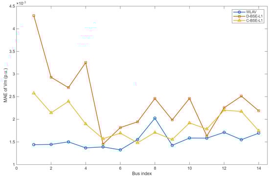
Figure 3. Voltage magnitude estimation results for the IEEE 14-bus system.

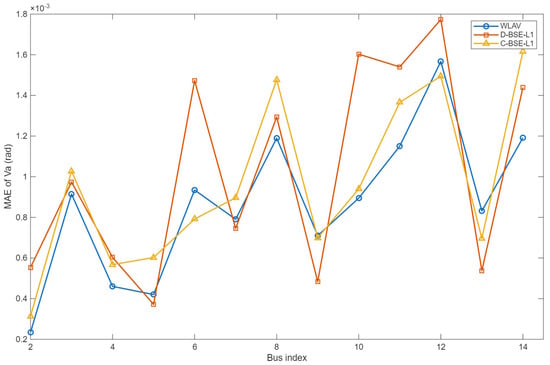
Figure 4. Voltage angle estimation results for the IEEE 14-bus system.

Table 1. Estimation results of D-BSE-L1.

Bus	Vm_True (p.u.)	Vm_Est (p.u.)	Va_True (Rad)	Va_Est (Rad)
1	1.060000	1.060883	0.000000	0.000000
2	1.045000	1.045554	−0.086963	−0.086826
3	1.010000	1.011155	−0.222095	−0.221795
4	1.017671	1.017706	−0.179994	−0.179760
5	1.019514	1.019632	−0.153133	−0.153052
6	1.070000	1.070317	−0.248202	−0.247685
7	1.061520	1.061661	−0.233169	−0.233383
8	1.090000	1.090181	−0.233169	−0.233272
9	1.055932	1.055837	−0.260726	−0.260937
10	1.050985	1.051663	−0.263497	−0.263565
11	1.056907	1.057392	−0.258145	−0.257848
12	1.055189	1.055005	−0.263119	−0.262930
13	1.050382	1.050687	−0.264527	−0.264713
14	1.035530	1.035192	−0.279840	−0.280431

Table 2. MAE of the state varibles.

	MAE of the State Varibles
SE methods	$V_i$	${\theta }_i$
D-BSE-L1	$2.19\times {10}^{-3}$	$9.08\times {10}^{-4}$
C-BSE-L1	$1.87\times {10}^{-3}$	$8.75\times {10}^{-4}$
WLAV	$1.53\times {10}^{-3}$	$8.10\times {10}^{-4}$

The results in Figure 3 and Figure 4 and Table 1 and Table 2 indicate that, in the IEEE 14-bus case, the three methods yield estimation errors of the same order of magnitude, with closely matched error magnitudes at the majority of buses. Moreover, the L1-based estimators maintain competitive accuracy under Gaussian noise. Relative to C-BSE-L1, the proposed D-BSE-L1 exhibits close agreement in both estimation trajectories and error profiles across buses, suggesting that the distributed solution reproduces the statistical performance of the centralized method without a material loss in accuracy. In addition, a side-by-side comparison between the bilinear-model results and those of the nonlinear WLAV benchmark shows similar overall MAEs, indicating that the bilinear approximation does not materially amplify modeling bias in this setting.

5.2. Robustness Test

To further assess the robustness and convergence performance of the proposed D-BSE-L1 estimator in the presence of bad data, this section compares it with the classical WLS + LNRT method on the IEEE 118-bus system. Three PMU phase angle measurements are randomly placed in each area, and bad data are injected by scaling a certain proportion of measurements to 1.5 or 5 times their true values. The estimation results of the two methods are shown in Figure 5, Figure 6, Figure 7 and Figure 8.

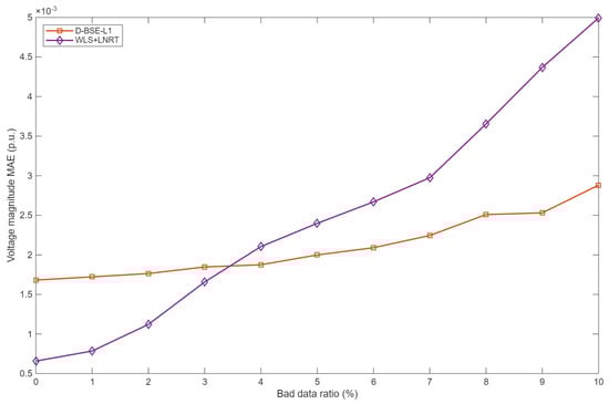
Figure 5. Voltage magnitude MAE under 1.5× bad data.

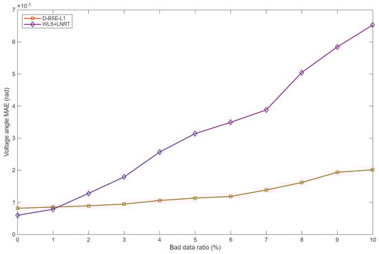
Figure 6. Voltage angle MAE under 1.5× bad data.

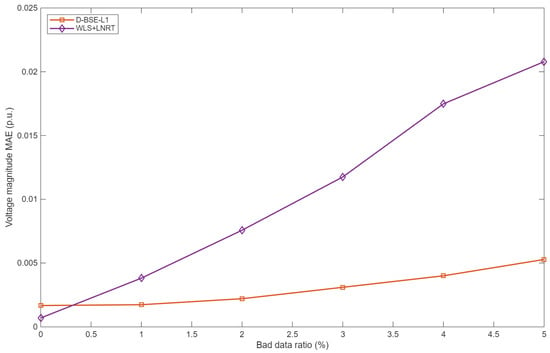
Figure 7. Voltage magnitude MAE under 5× bad data.

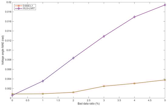
Figure 8. Voltage angle MAE under 5× bad data.

When the contamination ratio is small and outliers are moderate (for example, a few 1.5× bad data), the two methods exhibit very similar accuracy, and WLS + LNRT can even yield slightly smaller MAEs at some operating points. This behavior is consistent with classical robust estimation theory: under nearly Gaussian noise and rare bad data, quadratic loss estimators are statistically efficient, whereas L1-based estimators deliberately trade a slight loss in efficiency for improved robustness.

As either the contamination ratio or the outlier magnitude increases, D-BSE-L1 gradually becomes clearly superior. Once the bad-data ratio reaches about 4% at 1.5× or 1% at 5×, D-BSE-L1 already achieves smaller MAEs for both voltage magnitudes and angles. With 10% bad data at 1.5×, the voltage magnitude and voltage angle MAEs of D-BSE-L1 are about 62% and 54% of those of WLS + LNRT, respectively; with 5% bad data at 5×, the corresponding ratios further drop to approximately 43% and 51%. Over the tested range, the MAE curves in Figure 5, Figure 6, Figure 7 and Figure 8 diverge monotonically as the contamination level becomes more severe, confirming that the proposed estimator exhibits a much slower degradation of accuracy.

These robustness gains stem from the different ways in which residuals enter the objective. In D-BSE-L1, each residual appears in a weighted absolute-value term, so the influence of any single measurement grows only linearly with its error and remains effectively bounded. All measurements, including potential outliers, are handled within one convex optimization problem without explicit bad-data thresholds. In contrast, WLS+LNRT relies on a quadratic loss for estimation and then applies LNRT-based residual screening. The quadratic loss amplifies the impact of large residuals, and the fixed detection thresholds can lead to masking and swamping when multiple outliers are present, which explains the rapid growth of MAE for WLS+LNRT.

In this experiment, D-BSE-L1 also exhibits favorable computational performance. On the IEEE 118-bus system, it converges in about 0.5 s under the chosen stopping tolerance, whereas WLS + LNRT requires roughly an order of magnitude more CPU time. This difference is mainly due to the distributed bilinear formulation: D-BSE-L1 solves smaller area-wise subproblems whose coefficient matrices are factorized once via Cholesky decomposition and then reused in subsequent ADMM iterations, whereas WLS + LNRT repeatedly forms and factorizes large normal equations for the entire system and performs additional residual tests. Overall, Experiment 2 shows that D-BSE-L1 achieves a strong balance between robustness and computational efficiency under severe bad-data contamination.

5.3. Performance Test of State Estimators for Large-Scale Power Systems

To examine the scalability and computational efficiency of the proposed distributed framework on large-scale networks, we compare D-BSE-L1 with its centralized counterpart, C-BSE-L1, on a 1062-bus, 9-area test system. Each area is equipped with six randomly assigned PMU phase angle measurements. To ensure that the estimator still undergoes a nontrivial number of iterations, 2% of the measurements are corrupted by scaling them to twice their true values.

Figure 9 and Figure 10 summarize the area-wise estimation accuracies. For all regions, the MAEs of the voltage magnitude and angle produced by D-BSE-L1 and C-BSE-L1 are very close, indicating that distributing the computation over multiple areas does not noticeably degrade estimation quality, even in the presence of injected bad data. Thus, the proposed coordination scheme preserves the accuracy of the centralized bilinear formulation on this thousand-bus-scale system.

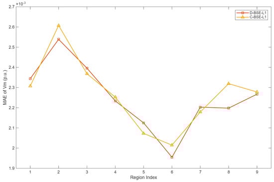
Figure 9. Voltage magnitude estimation accuracy for different areas in the 1062-Bus model.

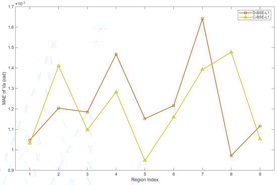
Figure 10. Voltage angle estimation accuracy for different areas in the 1062-Bus model.

In contrast, the runtime exhibits a clear difference. As reported in Table 3, D-BSE-L1 converges in 0.72 s, whereas C-BSE-L1 requires 2.46 s to reach the same convergence tolerance. In other words, the distributed implementation achieves the desired accuracy with only about 30% of the wall-clock time of the centralized method. The speed-up is mainly due to two factors. First, the distributed formulation decomposes the global linear systems into smaller area-wise problems, so the cost of each linear solve is significantly reduced. Second, in the third stage of D-BSE-L1, the symmetric positive-definite coefficient matrices are factorized once via Cholesky decomposition, and the factors are reused across ADMM iterations, so each subsequent update involves only inexpensive triangular solves. In the centralized case, the corresponding matrices are much larger, and repeated factorization leads to a higher overall computational burden.

Table 3. Times of CPU calculation.

	D-BSE-L1	C-BSE-L1
CPU times(s)	0.72	2.46

6. Conclusions

This paper proposes D-BSE-L1, a distributed robust state estimation method for the bilinear power system model that integrates a WLAV loss with ADMM-based area coordination. By reformulating the first-stage and third-stage subproblems as a convex quadratic program and a symmetric positive-definite linear system, respectively, and by exploiting cached Cholesky factorizations in the third stage, the method achieves a scalable, parallelizable computation framework without introducing additional robust loss hyperparameters.

Extensive simulations on the IEEE 14-, 118-, and 1062-bus systems demonstrate that D-BSE-L1 preserves the estimation accuracy of its centralized bilinear counterpart while significantly improving robustness to gross measurement errors and reducing computational time. On the IEEE 14-bus system, the distributed and centralized bilinear estimators produce nearly identical voltage magnitude and angle trajectories. On the IEEE 118-bus system, under severe bad-data contamination, D-BSE-L1 yields markedly smaller MAEs of voltage magnitudes and angles than the benchmark WLS+LNRT method for both moderate and large bad-data magnitudes. On the 1062-bus, 9-area system, D-BSE-L1 maintains the MAE of the centralized estimator while achieving a significantly shorter runtime through area-wise parallelization and cached factorization, indicating that the proposed framework provides an accurate, scalable, and outlier-robust solution for partitioned state estimation in large-scale power grids.

While the proposed method demonstrates superior robustness and efficiency, several directions merit further exploration. Future work will first focus on validating the effectiveness of D-BSE-L1 on real-world mixed SCADA-PMU datasets characterized by complex error patterns. Second, to address non-ideal communication conditions in distributed architectures (e.g., latency and packet loss), we intend to investigate asynchronous distributed optimization algorithms, thereby relaxing the strict requirements for synchronous communication.

References

- Blaabjerg, F.; Ma, K. Future on power electronics for wind turbine systems. IEEE J. Emerg. Sel. Top. Power Electron. 2013, 1, 139–152. [Google Scholar] [CrossRef]
- Farhangi, H. The path of the smart grid. IEEE Power Energy Mag. 2010, 8, 18–28. [Google Scholar] [CrossRef]
- Monticelli, A. State Estimation in Electric Power Systems: A Generalized Approach; Springer: Boston, MA, USA, 1999. [Google Scholar]
- Schweppe, F.C.; Wildes, J. Power system static-state estimation, part I: Exact model. IEEE Trans. Power Appar. Syst. 1970, PAS-89, 120–125. [Google Scholar] [CrossRef]
- Wu, F.F.; Moslehi, K.; Bose, A. Power system control centers: Past, present, and future. Proc. IEEE 2005, 93, 1890–1908. [Google Scholar] [CrossRef]
- Filho, M.B.D.C.; de Souza, J.C.S.; Glover, J.D. Roots, achievements, and prospects of power system state estimation: A review on handling corrupted measurements. Int. Trans. Electr. Energ. Syst. 2019, 29, e2779. [Google Scholar] [CrossRef]
- Gómez-Expósito, A.; Jaén, A.d.l.V.; Gómez-Quiles, C.; Rousseaux, P.; Van Cutsem, T. A taxonomy of multi-area state estimation methods. Electr. Power Syst. Res. 2011, 81, 1060–1069. [Google Scholar] [CrossRef]
- Xie, L.; Choi, D.-H.; Kar, S.; Poor, H.V. Fully distributed state estimation for wide-area monitoring systems. IEEE Trans. Smart Grid 2012, 3, 1154–1169. [Google Scholar] [CrossRef]
- Minot, A.; Lu, Y.; Li, N. A distributed gauss-newton method for power system state estimation. In Proceedings of the 2016 IEEE Power and Energy Society General Meeting (PESGM), Boston, MA, USA, 17–21 July 2016; IEEE: New York City, NY, USA, 2016; p. 1. [Google Scholar] [CrossRef]
- Zheng, W.; Wu, W. An adaptive distributed quasi-newton method for power system state estimation. IEEE Trans. Smart Grid 2019, 10, 5114–5124. [Google Scholar] [CrossRef]
- Cosovic, M.; Vukobratovic, D. Distributed gauss–newton method for state estimation using belief propagation. IEEE Trans. Power Syst. 2019, 34, 648–658. [Google Scholar] [CrossRef]
- Kekatos, V.; Giannakis, G.B. Distributed robust power system state estimation. IEEE Trans. Power Syst. 2013, 28, 1617–1626. [Google Scholar] [CrossRef]
- Zou, T.; Aljohani, N.; Wang, P.; Bretas, A.S.; Bretas, N.G. Bretas Distributed nonlinear state estimation using adaptive penalty parameters with load characteristics in the electricity reliability council of texas. J. Ind. Inf. Integr. 2021, 24, 100223. [Google Scholar] [CrossRef]
- Ho, C.H.; Wu, H.C.; Chan, S.C.; Hou, Y. A robust statistical approach to distributed power system state estimation with bad data. IEEE Trans. Smart Grid 2010, 11, 517–527. [Google Scholar] [CrossRef]
- Chen, T.; Cao, Y.; Sun, L.; Qing, X.; Zhang, J. A distributed robust power system state estimation approach using $t$-distribution noise model. IEEE Syst. J. 2021, 15, 1066–1076. [Google Scholar] [CrossRef]
- Chen, T.; Liu, F.; Li, P.; Sun, L.; Amaratunga, G.A.J. A distributed multi-area power system state estimation method based on generalized loss function. Meas. Sci. Technol. 2023, 34, 115010. [Google Scholar] [CrossRef]
- Lin, C.; Wu, W.; Guo, Y. Decentralized robust state estimation of active distribution grids incorporating microgrids based on PMU measurements. IEEE Trans. Smart Grid 2020, 11, 810–820. [Google Scholar] [CrossRef]
- Zhang, Z.; Ju, Y. An Embedded Consensus ADMM Distribution Algorithm Based on Outer Approximation for Improved Robust State Estimation of Networked Microgrids. J. Mod. Power Syst. Clean Energy 2024, 12, 1217–1226. [Google Scholar] [CrossRef]
- Gomez-Exposito, A.; Gomez-Quiles, C.; Jaen, A.d.l.V. Bilinear power system state estimation. IEEE Trans. Power Syst. 2012, 27, 493–501. [Google Scholar] [CrossRef]
- Gomez-Quiles, C.; Gil, H.A.; Jaen, A.d.l.V.; Gomez-Exposito, A. Equality-constrained bilinear state estimation. In Proceedings of the 2013 IEEE Power & Energy Society General Meeting, Vancouver, BC, Canada, 21–25 July 2013; IEEE: New York City, NY, USA, 2013; p. 1. [Google Scholar] [CrossRef]
- Chen, Y.; Ma, J.; Liu, F.; Mei, S. A bilinear robust state estimator: Bilinear robust state estimator. Int. Trans. Electr. Energy Syst. 2016, 26, 1476–1492. [Google Scholar] [CrossRef]
- Parsegov, S.; Kubentayeva, S.; Gryazina, E.; Gasnikov, A.; Ibáñez, F. ADMM-based distributed state estimation for power systems: Evaluation of performance. IFAC Pap. 2020, 53, 182–188. [Google Scholar] [CrossRef]
- Im, J.; Ban, J.; Kim, Y.-J.; Zhao, J. PMU-based distributed state estimation to enhance the numerical stability using equality constraints. IEEE Trans. Power Syst. 2024, 39, 4409–4421. [Google Scholar] [CrossRef]
Disclaimer/Publisher’s Note: The statements, opinions and data contained in all publications are solely those of the individual author(s) and contributor(s) and not of MDPI and/or the editor(s). MDPI and/or the editor(s) disclaim responsibility for any injury to people or property resulting from any ideas, methods, instructions or products referred to in the content. |
© 2025 by the authors. Licensee MDPI, Basel, Switzerland. This article is an open access article distributed under the terms and conditions of the Creative Commons Attribution (CC BY) license (https://creativecommons.org/licenses/by/4.0/).