Enhancing Extrapolation of Buckley–Leverett Solutions with Physics-Informed and Transfer-Learned Fourier Neural Operators

Abstract

Accurate modeling of multiphase flow in porous media remains challenging due to the nonlinear transport and sharp displacement fronts described by the Buckley–Leverett (B-L) equation. Although Fourier Neural Operators (FNOs) have recently emerged as powerful surrogates for parametric partial differential equations, they exhibit limited robustness when extrapolating beyond the training regime, particularly for shock-dominated fractional flows. This study aims to enhance the extrapolative performance of FNOs for one-dimensional B-L displacement. Analytical solutions were generated using Welge’s graphical method, and datasets were constructed across a range of mobility ratios. A baseline FNO was trained to predict water saturation profiles and evaluated under both interpolation and extrapolation conditions. While the standard FNO accurately reconstructs saturation profiles within the training window, it misestimates shock positions and saturation jumps when extended to longer times or higher mobility ratios. To address these limitations, we develop Physics-Informed FNOs (PI-FNOs), which embed PDE residuals and boundary constraints, and Transfer-Learned FNOs (TL-FNOs), which adapt pretrained operators to new regimes using limited data. Comparative analyses show that both approaches markedly improve extrapolation accuracy, with PI-FNOs achieving the most consistent and physically reliable performance. These findings demonstrate the potential of combining physics constraints and knowledge transfer for robust operator learning in multiphase flow systems.

1. Introduction

The B-L equation [1] is a classical model for immiscible, incompressible two-phase displacement in porous media. Owing to its analytical tractability, the B-L model remains a fundamental tool in reservoir engineering, both for understanding displacement mechanisms and for designing recovery processes. For instance, the B-L formulations are central in screening studies for waterflooding, and with modifications to the fractional-flow function, also serve as proxies for chemical flooding as well as for gas injection [2,3,4,5].

A key feature of the B-L solution is the development of a shock front, representing the abrupt transition between the displaced and displacing phases. Accurately capturing this front is essential for predicting breakthrough times, estimating sweep efficiency, and optimizing injection strategies in oilfield reservoir management. Traditionally, the B-L equation has been addressed using analytical methods (e.g., Welge’s graphical method, method of characteristics) and numerical schemes (e.g., finite difference, finite volume). Analytical solutions are limited to idealized cases, while numerical solvers must use sufficiently fine grids to resolve saturation shocks, or else numerical diffusion and spurious oscillations degrade their accuracy. This has motivated the development of machine learning surrogates that are both computationally efficient and physically consistent [6,7,8].

Physics-Informed Neural Networks (PINNs) [9] have emerged as a promising approach to enforce governing equations in data-driven models. Several studies have applied PINNs to solve the B-L equation. Diab et al. [10] proposed data-free and data-efficient PINN variants, leveraging attention mechanisms and hard enforcement of boundary/initial conditions to improve robustness in shock-dominated flows. Fraces et al. [11] developed a hybrid PINN-GAN (Generative Adversarial Network) framework for forward and inverse B-L problems, demonstrating that sparse observations combined with physics constraints enable recovery of fractional-flow parameters and shock-front dynamics. Zhang et al. [12] introduced a Transformer-based PINN in which self-attention improves the resolution of nonlinear shocks across mobility-ratio regimes. Almajid and Abu-Al-Saud [13] implemented PINNs via DeepXDE (v1.11.0) for forward and inverse B-L problems, showing reasonable accuracy in gas–water displacement. More recently, Ma et al. [14] extended the physics-informed paradigm by proposing GAN-based surrogates (PIG-GAN and DI-GAN), embedding the B-L residuals into both generator and discriminator losses. Their framework achieved accurate front predictions in forward and inverse tasks, even under noisy conditions. Collectively, these studies demonstrate the potential of PINNs to incorporate physical mechanism into neural models of the B-L fractional flow, while also highlighting the persistent difficulty of resolving discontinuous shocks and achieving reliable extrapolation.

Parallel to PINNs, neural operator learning has emerged as a resolution-invariant surrogate paradigm. The FNOs introduced by Li et al. [15] learns mappings between infinite-dimensional function spaces via spectral convolution, providing global receptive fields and grid-invariant generalization. FNOs have achieved state-of-the-art performance across diverse PDEs, including Darcy flow, Burgers/advection, heat field reconstruction, weather forecasting, turbulence flow, and geological carbon storage [16,17,18,19,20]. However, although FNOs excel at interpolation and zero-shot super-resolution, they still face notable limitations in extrapolating beyond their training distribution, particularly in unseen parameter regimes, out-of-distribution spatial or temporal domains, and tasks requiring generalization to significantly different initial/boundary conditions [21,22,23].

For the B-L problem, extrapolation arises when extending predictions to longer horizons and different mobility ratios. In such cases, vanilla FNOs often mis-predict shock arrival times, under- or overestimate saturation profiles. This extrapolation gap motivates targeted remedies. Three complementary strategies have been developed to enhance the extrapolation capability of FNOs [23]. First, Physics-Informed FNOs (PI-FNOs) augment training with PDE residuals and boundary/initial conditions, thereby regularizing the operator toward physically consistent extrapolation [24,25]. Second, Transfer-Learned FNOs (TL-FNOs) fine-tune a pre-trained operator on small target datasets, enabling efficient adaptation across regimes with substantially fewer labeled samples [26,27]. In addition, Multi-Fidelity FNOs (MF-FNOs) integrate inexpensive low-fidelity data with limited high-fidelity data, leveraging information across fidelities to improve predictive accuracy and reduce training costs under distribution shifts [20,28,29]. The strategies show promise, but their relative merits in shock-dominated extrapolation problems remain insufficiently quantified. Such problems are uniquely challenging because small perturbations in input parameters or boundary conditions can trigger large discrepancies in shock location, front speed, and breakthrough time.

In this study, we investigate the extrapolation of the B-L solution using Physics-Informed and Transfer-Learned FNOs. The main contributions of this work are as follows:

• We formalize extrapolation regimes for the B-L problem, including temporal extension and mobility-ratio shifts.
• We develop a Physics-Informed FNO (PI-FNO) that embeds the B-L residuals into the learning process.
• We design a Transfer-Learned FNO (TL-FNO) framework capable of adaptation under limited target samples.
• We present a comprehensive comparative study on one-dimensional B-L benchmarks.

The remainder of this paper is organized as follows. Section 2 reviews the B-L equation and outlines the foundations of FNOs, PINNs, PI-FNOs, and TL-FNOs. Section 3 describes the problem setup, defines the extrapolation regimes, and presents numerical experiments on one-dimensional B-L benchmarks, including comparative performance analyses. Section 4 concludes the paper.

2. Materials and Methods

2.1. Mathematical Formulation of the B-L Equation

The B-L equation is derived from the conservation of mass for the displacing phase (e.g., water) and the Darcy’s law for multiphase flow. Consider 1D, horizontal, immiscible, incompressible two-phase (water-oil) flow in a homogeneous porous medium with constant porosity ϕ and cross-sectional area A. Let S_w be water saturation, S_o = 1 − S_w oil saturation. Denote volumetric flow rates (through the cross-section) by q_α for phase α ∈ {w, o}, and the total flow rate q_T = q_w + q_o. Assuming that capillary pressure and gravity are neglected. The fluid flow equations could be simplified to the following [2]:

$$\varnothing {\displaystyle \frac{\mathsf{\partial }{S}_w}{\mathsf{\partial }t}}+{\displaystyle \frac{1}{A}}{\displaystyle \frac{\mathsf{\partial }{q}_w}{\mathsf{\partial }t}}=0$$

(1)

$$q_{\alpha }=-{\displaystyle \frac{Ak{k}_{r\alpha }}{{\mu }_{\alpha }}}{\displaystyle \frac{\mathsf{\partial }P}{\mathsf{\partial }x}}$$

(2)

where k is absolute permeability, $k_{r\alpha }$ is relative permeability of phase α, ${\mu }_{\alpha }$ viscosity, porosity ϕ, and P is reservoir pressure. Define phase mobilities:

$${\lambda }_{\alpha }={\displaystyle \frac{k_{r\alpha }}{{\mu }_{\alpha }}}$$

(3)

and total mobility of water and oil:

$${\mathsf{\lambda }}_{\mathrm{T}}={\mathsf{\lambda }}_{\mathrm{o}}+{\mathsf{\lambda }}_{\mathrm{w}}$$

(4)

In the context of immiscible displacement such as waterflooding, the mobility ratio M is defined as the ratio of the displacing-phase mobility (water) to the displaced-phase mobility (oil):

$$M={\displaystyle \frac{{\mathsf{\lambda }}_{\mathrm{w}}}{{\mathsf{\lambda }}_{\mathrm{o}}}}={\displaystyle \frac{k_{rw}/{\mu }_w}{k_{ro}/{\mu }_o}}$$

(5)

A mobility ratio M > 1 indicates an unfavorable displacement, often leading to viscous fingering and early water breakthrough, while M < 1 corresponds to a favorable displacement with more stable flood fronts.

Under the standard B-L assumptions, the fractional-flow of water is defined as the ratio of water mobility to that of total mobility and is written as:

$$f_w(S_w)={\displaystyle \frac{{\lambda }_w}{{\lambda }_T}}={\displaystyle \frac{1}{1+\frac{k_{ro}{\mu }_w}{k_{rw}{\mu }_o}}}$$

(6)

We use Corey-type relative permeability functions [30]. Specifically, the relative permeability functions of water and oil phases are written as:

$$k_{rw}=k_{rw,max}{\left({\displaystyle \frac{S_w-S_{wc}}{1-S_{wc}-S_{or}}}\right)}^{n_w}$$

(7)

$$k_{ro}=k_{ro,max}{\left({\displaystyle \frac{1-S_w-S_{or}}{1-S_{wc}-S_{or}}}\right)}^{n_o}$$

(8)

$k_{ri,max}$ is the maximum relative permeability value of phase $i$, and $n_i$ is the relative permeability exponent of phase $i$. With a constant total flow rate, Equation (1) reduces to the scalar conservation law:

$${\displaystyle \frac{\mathsf{\partial }{S}_w}{\mathsf{\partial }t}}+{\displaystyle \frac{q_T}{\varphi A}}{\displaystyle \frac{\mathsf{\partial }{f}_w\left(S_w\right)}{\mathsf{\partial }x}}=0$$

(9)

For a classical waterflood with initial condition and boundary condition are provided as follows:

Initial condition:

$$S_w(x, t=0)=S_{wi}$$

(10)

Boundary condition:

$$S_w(x=0, t)=S_{inj}$$

(11)

where S_wi is initial water saturation, and S_inj is injected water saturation.

To facilitate solving the B-L equation, Equation (9) can be transformed into a dimensionless form as follows:

$${\displaystyle \frac{\mathsf{\partial }{S}_w}{\mathsf{\partial }{t}_D}}+{\displaystyle \frac{\mathsf{\partial }{f}_w}{\mathsf{\partial }{x}_D}}=0$$

(12)

In Equation (12), the dimensionless time, $t_D$ and dimensionless distance $x_D$, are introduced and defined as:

$$t_D={\displaystyle \frac{q_T}{\mathsf{\varphi }AL}}t{ x}_D={\displaystyle \frac{x}{L}}$$

(13)

where L is the length. Using the dimensionless time and distance, the residual of the B-L equation is defined as:

$$R={\displaystyle \frac{\mathsf{\partial }{S}_w}{\mathsf{\partial }{t}_D}}+{\displaystyle \frac{\mathsf{\partial }{f}_w\left(S_w\right)}{\mathsf{\partial }{x}_D}}$$

(14)

2.2. Welge’s Graphical Method

Welge’s graphical method, introduced in 1952, represents an important extension and practical tool of the B-L waterflooding theory [7]. By transforming the nonlinear differential form of the governing equation into a linear construction and employing graphical techniques, it simplifies the computational procedure for analyzing immiscible displacement. By drawing a tangent from the initial water saturation S_wi to the fractional-flow curve, the shock saturation $S_w^{*}$ is determined as shown in Figure 1. Although numerous refinements of Welge’s method have been proposed over the years, our use of the classical formulation is limited to generating benchmark solutions for neural operator training and evaluation. A detailed comparison with modified Welge approaches is beyond the scope of the present work, which focuses on extrapolative performance of learning-based operators.

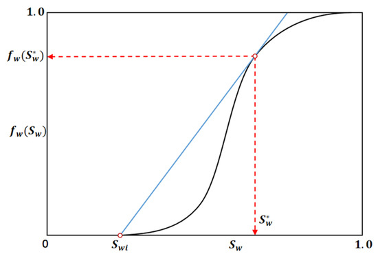
Figure 1. Schematic of Welge’s graphical method for the B-L equation. The tangent to the fractional-flow curve defines the shock saturation, enabling direct calculation of shock velocity and breakthrough time.

The corresponding shock-front velocity is then given by:

$$v_s={\displaystyle \frac{f_w\left(S_w^{*}\right)-f_w\left(S_{wi}\right)}{S_w^{*}-S_{wi}}}$$

(15)

which quantifies the propagation speed of discontinuity. The position x_f of the shock front can be expressed as:

$$x_f={\displaystyle \frac{q_T}{A\mathsf{\varphi }}}·t·v_s$$

(16)

This provides a direct means of estimating both the speed of the advancing displacement front and the breakthrough time, obtained by dividing the distance to the producer by the velocity v_s. In this way, Welge’s construction enables practical and efficient prediction of dynamic waterflood behavior.

A MATLAB (6.0) implementation of Welge’s graphical method, as provided in the Appendix of Wu’s work [31], was used to numerically evaluate the analytical Buckley–Leverett solution. Figure 2 presents the water saturation profiles along the dimensionless distance at several dimensionless times.

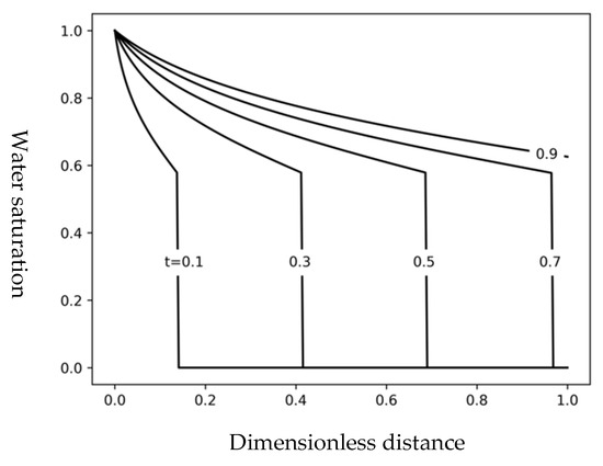
Figure 2. Water saturation profiles versus dimensionless distance at several dimensionless times (t = 0.1, 0.3, 0.5, 0.7, 0.9) for the B-L displacement, with sharp discontinuities separating the injected and displaced fluids.

2.3. Fourier Neural Operator (FNO)

Let G: A→U denote the solution operator mapping input functions (initial/boundary data, coefficients such as permeability k(x), ϕ(x), mobility ratio M) to the PDE solution (e.g., S_w(x,t)). Neural operators learn a parametric approximation G_θ directly in function space, aiming for resolution invariance: once trained, G_θ can be evaluated on different meshes without retraining.

The FNO approximates G by composing spectral convolution layers with pointwise affine maps:

1.

Lifting: embed inputs a(x) (e.g., S_w(x, t), M) to a higher dimensional space by a fully connected neural network P:

$$v_0\left(x\right)=P\left[a\right]\left(x\right),$$

(17)

2.

Spectral transformations: a sequence of transformations in Fourier space (ℓ = 0, …, L–1) is applied to the lifted function $v_0\left(x\right)$ The output at the (ℓ + 1)-th stage of the FNO is then given by:

$$v_{l+1}\left(x\right)=\sigma \left(W\left[v_l\right]\left(x\right)+K\left(\theta \right)\left[v_l\right]\left(x\right)\right),$$

(18)

where $\sigma$ denotes a nonlinear activation function. W is the linear transform. The kernel integral operator K is parameterized by θ and defined in Fourier space:

$$K\left(\theta \right)\left[v_l\right]\left(x\right)=F^{-1}\left[R_{\theta }·F\left[v_l\right]\right]\left(x\right).$$

(19)

where F and F⁻¹ denote the Fourier transform and inverse Fourier transform, $R_{\theta }$ is a vector of learned Fourier coefficients.

Equation (19) plays a central role by linking the PDE input parameters to their spectral representation, thereby capturing the underlying physical structure in Fourier space. In practice, when both the input and output fields are sufficiently smooth, their Fourier coefficients decay rapidly, which enables efficient representation with only a limited set of modes. By imposing a cutoff on the maximum number of retained Fourier modes, the operator can be approximated within a finite-dimensional basis, yielding a compact yet expressive parameterization.

3.

Projection: map v_L(x) back to the target field via a linear head Q.

Through this sequence of lifting, spectral transformations, and projection, the FNO builds a compact finite-dimensional representation of the underlying operator, which serves as the basis for its efficiency and generalization. Leveraging this representation, the FNO learns directly from PDE input–output pairs and can rapidly predict solutions under varying initial and boundary conditions or different coefficients. Once trained, it generalizes well to unseen parameter regimes, delivering orders-of-magnitude speedups compared with finite-difference or finite-volume solvers [22]. In addition, its resolution-invariant design enables direct evaluation on finer grids (zero-shot super-resolution), while the spectral formulation allows efficient capture of long-range dependencies and has demonstrated scalability in large-scale turbulent and climate simulations [18,19].

2.4. Physics Informed Neural Networks (PINNs)

PINNs incorporate the residuals of governing PDEs, together with penalties for initial and boundary conditions, directly into their loss function [9,32]. Leveraging the automatic differentiation capabilities of modern deep learning frameworks, PINNs efficiently compute the required spatial and temporal derivatives to evaluate PDE residual errors during training. This approach enforces physical consistency while offering mesh-free training, data efficiency in sparse regimes, and flexibility for complex geometries. Despite their promise, vanilla PINNs face well-documented challenges when applied to hyperbolic conservation laws such as the B-L equation. First, they are affected by spectral bias, which favors low-frequency modes and leads to excessive smoothing of sharp saturation discontinuities; this often causes inaccurate shock positions, smeared profiles, or non-physical oscillations, and requires additional remedies such as entropy-consistent formulations or incorporate a diffusive term to stabilize training [10,11]. Second, standard PINNs are typically problem-specific solvers: once trained for a given set of initial and boundary conditions (IC/BC) or mobility ratios, they must be retrained to handle new regimes, limiting their utility as general-purpose surrogate models [22]. This motivates exploring physics-informed operator-learning alternatives, which are designed to learn mappings across function spaces.

2.5. Physics-Informed Operator Learning

While FNOs demonstrate strong accuracy for many PDEs, their extrapolative reliability diminishes in hyperbolic transport problems such as the B-L equation, where shocks and discontinuities dominate. To improve the extrapolative capability of the baseline FNO, we incorporate physical constraints from the governing Buckley–Leverett (B-L) equation into the training objective [24,25]. In the Physics-Informed FNO (PI-FNO), the loss function combines contributions from supervised data pairs, PDE residuals, and boundary/initial conditions:

$$L=L_{data}+{\omega }_1{L}_{res}+{\omega }_2{L}_{BC}+{\omega }_3{L}_{IC}.$$

(20)

L_data measures discrepancies with available labeled solutions, while the residual term L_res enforces the B-L conservation law at collocation points. The initial (L_IC) and additional boundary (L_BC) penalties constrain the network to honor physical conditions. ${\mathsf{\omega }}_1$, ${\mathsf{\omega }}_2$, ${\mathsf{\omega }}_3$ are weighting parameters controlling the relative importance of each term. Their values are determined by a combination of normalization—ensuring each term contributes on comparable scales and empirical tuning to achieve stable convergence. In this study, we select ${\omega }_1=1$, ${\omega }_2=10$, and ${\omega }_3=1$, providing a balance between accurate data fitting and enforcement of the B-L physical constraints.

L_res is expressed as:

$$L_{res}={\displaystyle \frac{1}{N_r}}{\displaystyle {\sum }_{i=1}^{N_r}}{\left[{\displaystyle \frac{\mathsf{\partial }{u}_{\theta }}{\mathsf{\partial }t}}(x_i,t_i)+{\displaystyle \frac{\mathsf{\partial }{f}_w\left(u_{\theta }\right(x_i,t_i\left)\right)}{\mathsf{\partial }x}}\right]}^2.$$

(21)

$u_{\theta }\left(x_i, t_i\right)$ denotes the FNO-predicted water saturation at spatial location $x_i$ and time $t_i$, where $\theta$ represents the trainable parameters of the neural operator, and $f_w\left(u_{\theta }\right)$ is the fractional flow function used in the B-L equation, whose explicit form is provided earlier in Equation (6).

The PDE residual term is computed using automatic differentiation, enabling efficient evaluation of the nonlinear fractional-flow derivative and implicitly enforcing the conservation structure of the governing equation. By penalizing deviations from the B-L equation, PI-FNO reduces shock smearing and prevents nonphysical saturation evolution.

2.6. Transfer-Learned FNO

In addition to physics-informed regularization, another promising strategy to enhance extrapolation of FNOs is to leverage transfer learning operator learning. These approaches exploit either knowledge from pre-trained models to improve performance under distribution shifts while reducing training cost.

The TL-FNO framework assumes the existence of a source model ${ G}_{{\theta }_s}$, pre-trained on a broad or related distribution of B-L solutions. This model is adapted to a target regime (e.g., new mobility ratio, or temporal extension) by fine-tuning part of the network with limited target data. Figure 3 outlines the TL-FNO framework. A source FNO is first trained on B-L solutions at a reference regime (M = 2).

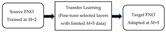
Figure 3. Schematic of the TL-FNO framework.

Knowledge from the pretrained model is then reused, and selected layers are fine-tuned with limited target samples at a different regime (M = 5). The adapted TL-FNO reduces data requirements and training cost while improving extrapolative accuracy compared with training a new model from scratch.

Equation (22) defines the data-driven transfer-learning loss used to adapt the pretrained operator $G_{{\theta }_s }$ to the target regime. For each training sample $a_i\left(x\right)$, the operator $G_{\theta }\left(a_i\left(x\right)\right)$ outputs the predicted water saturation field at time $t_i$. This prediction is compared with the corresponding target saturation field $S_w^{\mathrm{target}}(x_i,t_i)$. The loss is computed as the mean squared error over all $N_d$ labeled samples in the target dataset:

$$L_{TL-FNO}={\displaystyle \frac{1}{N_d}}{\sum }_{i=1}^{N_d}{\left[G_{\theta }\left(a_i\left(x\right)\right)-S_w^{target}(x_i, t_i)\right]}^2.$$

(22)

This objective adjusts the trainable parameters $\theta$ (typically a subset of the pretrained weights) so that the operator’s predictions match the target-domain solutions. In essence, the loss measures how well the adapted FNO reproduces the B-L saturation profiles for the new mobility-ratio regime using limited target data.

Different transfer strategies can be employed:

• Full fine-tuning: update all parameters from a pre-trained operator.
• Partial freezing: retain most pretrained weights but selectively update the lifting, projection, and possibly subsets of the Fourier layers. The choice of which layers to fine-tune is determined empirically through numerical experiments, balancing accuracy and computational efficiency [27].
• Low-rank adapters: apply a low rank decomposition to the weight matrices, introducing trainable low-rank matrices while keeping the original weights fixed. This reduces memory and computational cost while preserving accuracy during fine-tuning [33].

In this work, we employ the partial freezing strategy, which preserves the operator structure learned from the source regime while providing sufficient flexibility to adapt to the target mobility ratios using limited data. This approach reduces the dependence on large, labeled datasets and enables efficient generalization to unseen B-L regimes with minimal computational overhead.

3. Results and Discussion

To demonstrate the effectiveness of Physics-Informed and Transfer-Learned FNOs in handling shock-dominated transport, we consider the one-dimensional B-L displacement problem as a representative benchmark. This case offers a well-understood analytical structure while exhibiting strong nonlinearities and sharp saturation fronts that pose challenges for extrapolation. The numerical experiments are designed to assess the ability of different operator-learning frameworks to generalize beyond the training regime in extended time horizons and altered mobility ratios. By comparing the baseline FNO with its physics-informed and transfer-learning extensions, we highlight how these strategies improve predictive accuracy, shock-front tracking, and data efficiency in scenarios where conventional FNOs typically fail.

3.1. Problem Setup

Numerical experiments were conducted on a one-dimensional homogeneous reservoir model of 100 m length in the x-direction, with the formation and fluid parameters summarized in Table 1. The endpoint mobility ratio M = 2 was determined from the corresponding relative permeability and viscosity values listed in Table 1. Using these parameters, analytical B-L solutions were generated via Welge’s graphical method. For the baseline FNO, For the baseline FNO, a dataset of 2048 observation pairs ${\left\{a_i\left(x\right),u_i\left(x\right)\right\}}_{i=1}^{2048}$ was used, where $a_i\left(x\right)$ denotes the $i$-th sample of the input field $a\left(x\right)$, representing initial water saturation, u_i(x) represents the corresponding water saturation at a later specified time. These pairs are partitioned into 1248 training, 400 validation, and 400 testing samples. The training interval was restricted to [0.5, 2.0] days, while validation and testing extended to [2.0, 5.0] days, enabling assessment of temporal extrapolation. All training data were generated on a standard workstation equipped with an Intel i7 CPU (3.4 GHz) and 32 GB of RAM. The input dataset is a tensor (N_T, N_X, N_C), where N_T = 2048 (time steps), N_X = 8192 (spatial discretization), and N_C = 2 (channels: water saturation, time).

Table 1. Reservoir and fluid properties used in the one-dimensional homogeneous B-L problem.

Parameter	Value	Unit
Cross-section area, $A$	1	m2
Length of formation, $L$	100	m
Injection rate, $q_T$	10−4	m3/s
Injection time, $t$	2	days
Water viscosity, ${\mu }_w$	1.0	mPa · s
Oil viscosity, ${\mu }_o$	2.0	mPa · s
Injection water saturation, $S_{inj}$	1.0	-
Initial water saturation, $S_{wj}$	0.0	-
Maximum relative permeability of water, $k_{rw,max}$	0.80	-
Maximum relative permeability of oil, $k_{ro,max}$	0.80	-
Relative permeability exponent of water, $n_w$	2.0	-
Relative permeability exponent of oil, $n_o$	2.0	-

A FNO is trained to predict the saturation profile at the next time step given the current profile. During training, inputs are lifted into a higher-dimensional space, transformed through stacked spectral layers where Fourier coefficients are updated, and projected back to the physical domain to yield predictions. The model parameters are optimized by minimizing the mean-squared error between predictions and reference solutions via Adam optimizer. Once trained, the FNO predicts full saturation profiles in under 1 ms, representing a 10~100 times speedup compared with a conventional finite-difference Buckley–Leverett solver.

3.2. Baseline FNO Performance

We establish a baseline using the FNO trained purely on data without physics or transfer-learning enhancements. The model was trained on the training dataset, with the training set covering time intervals up to 2 days and a fixed mobility ratio of M = 2. Evaluation was performed both within the training regime (interpolation) and beyond it (extrapolation to longer times and different mobility ratios). Figure 4 shows that the baseline FNO demonstrates strong interpolation performance, accurately reproducing the water saturation profiles and capturing the rarefaction and displacement fronts. Comparison with the analytical B-L solution (blue solid line) confirms excellent agreement within the training regime.

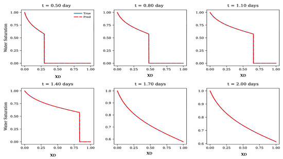
Figure 4. Comparison of baseline FNO predictions (red dashed lines) with analytical Buckley–Leverett solutions (blue solid lines) at different times. The model accurately reproduces water saturation profiles and displacement fronts within the training regime, demonstrating strong interpolation capability. For clarity, the saturation range is adjusted to [0.6, 1] at later times (t = 1.7 and t = 2.0 days) to highlight subtle differences between the predicted and analytical profiles near breakthrough.

The coefficient of determination (R²), mean squared error (MSE) and mean absolute error (MAE) are used to quantify the difference between the predicted and analytical saturation profiles. The coefficient $R^2$ is defined as:

$$R^2=1-{\displaystyle \frac{{\sum }_i(y_i-{\widehat{y}}_i{)}^2}{{\sum }_i(y_i-\stackrel{-}{y}{)}^2}}.$$

(23)

where $y_i$ denotes the reference saturation values, ${\widehat{y}}_i$ the predicted values, and $\stackrel{-}{y}$ their mean. A value of $R^2$ close to 1 indicates strong agreement between the predicted and analytical solutions.

Table 2 summarizes the interpolation accuracy of the baseline FNO across different time snapshots within the training regime. The model achieves consistently high correlation with the analytical B-L solution, with $R^2=0.999$ for all cases. Both MSE and MAE remain extremely small, indicating that the FNO almost perfectly reconstructs the saturation profiles and accurately captures the sharp displacement fronts. Although MSE and MAE show a slight increasing trend as time approaches breakthrough (e.g., at $t=1.7$ and $t=2.0$ days), the errors remain negligible and do not affect the overall shape or position of the saturation front. These results demonstrate that the baseline FNO performs exceptionally well in the interpolation regime and provides a reliable reference point for evaluating extrapolative performance in later sections.

Table 2. Interpolation accuracy of baseline FNO at different times.

Time (Days)	R2	MAE	MSE
0.5	0.999	1.8 × 10−4	1.2 × 10−7
0.8	0.999	4.5 × 10−5	3.6 × 10−9
1.1	0.999	5.0 × 10−5	2.9 × 10−9
1.4	0.999	4.9 × 10−5	3.9 × 10−9
1.7	0.999	1.1 × 10−4	1.7 × 10−8
2.0	0.999	1.4 × 10−4	3.9 × 10−8

Yet, in the extrapolation regime, the limitations of a purely data-driven FNO become evident as demonstrated in Figure 5. Figure 5 illustrates the baseline FNO predictions compared against analytical B-L solutions at times extending beyond the training window [0.5, 2.0] days, and the accuracy trends are quantified in Table 3, together demonstrating the model’s strong interpolation capability but limited reliability in extrapolation. At t = 2.0 days, within the trained temporal domain, the FNO reproduces the saturation profile with near-perfect accuracy (R² ≈ 1.0). Even so, as time progresses beyond t = 2.0 days, the predictions gradually deviate from the analytical solutions. At t = 2.6 days, the deviation remains minor, but from t = 3.2 days onward, noticeable discrepancies emerge, the predicted front becomes steeper near the inlet and shallower near the outlet. By t = 3.8~5.0 days, the predicted saturation front lags markedly behind the analytical solution, reflecting accumulated temporal errors and a loss of physical consistency, with the R² dropping below 0.5 at t = 5.0 days. Moreover, the MSE and MAE increase consistently with time, demonstrating that whereas the FNO is an efficient interpolator, it lacks robustness for long-term extrapolation of nonlinear hyperbolic B-L.

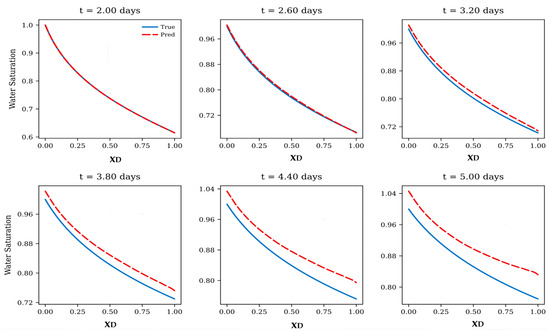
Figure 5. Baseline FNO predictions compared with analytical B-L solutions for extrapolation beyond the training window [0.5, 2.0] days. The model interpolates accurately at t = 2.0 days but exhibits progressive degradation at later times.

Table 3. Extrapolation accuracy of the baseline FNO beyond the training window [0.5, 2.0] days. The metrics R², MSE, and MAE are reported for successive times up to 5.0 days, illustrating the progressive loss of accuracy as the prediction horizon extends.

Time (Days)	R2	MAE	MSE
2.0	0.999	1.45 × 10−4	3.05 × 10−8
2.6	0.998	3.31 × 10−3	1.32 × 10−5
3.2	0.976	1.23 × 10−2	1.55 × 10−4
3.8	0.886	2.49 × 10−2	6.22 × 10−4
4.4	0.697	3.73 × 10−2	1.42 × 10−3
5.0	0.415	4.81 × 10−2	2.39 × 10−3

Figure 6 presents baseline FNO predictions when the mobility ratio is shifted from the training condition of M = 2 to M = 5. As demonstrated, at early times (t = 0.5~1.1 days), the model captures the overall trend but fails to reproduce the sharp saturation front characteristic of higher mobility ratios, leading to smoother and prematurely advanced predictions. As time progresses (t = 1.4–2.0 days), the discrepancy increases, with the model consistently overestimating water saturation across the domain. The predicted front becomes diffused and lags in representing the strong nonlinear displacement behavior present in the analytical solution.

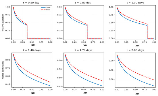
Figure 6. Baseline FNO predictions versus analytical B-L solutions when the mobility ratio shifts from the training regime (M = 2) to M = 5.

Figure 5 and Figure 6 collectively highlight the limitations of the baseline FNO in extrapolation. In the temporal domain (Figure 5), the model reproduces saturation profiles accurately within the training window but progressively loses accuracy at later times. In the parameter domain (Figure 6), the shift from M = 2 to M = 5 further exposes the model’s weaknesses, as it fails to generalize to more unstable displacement conditions, yielding significant errors in water saturation. Together, these results confirm that while the FNO is a powerful interpolator, it lacks robustness for extrapolation in both time and parameter space, motivating the introduction of physics-informed and transfer-learning strategies.

Table 4 summarizes the extrapolation performance of the baseline FNO when the mobility ratio is shifted from the training regime ($M=2$) to $M=5$. Unlike the interpolation case, the accuracy deteriorates noticeably as time increases. Although the model maintains relatively high fidelity at early times ($R^2>0.97$ for $t=0.5$~0.8 days), the predictive capability drops sharply beyond $t=1.1$ days, with $R^2$ falling to 0.478 by $t=2.0$ days. The increasing MSE and MAE indicate cumulative errors in saturation magnitude, consistent with the observed smoothing of the displacement front. These results demonstrate that the baseline FNO struggles to generalize across mobility ratios, underscoring the need for physics-informed constraints or transfer learning to achieve reliable extrapolation in more unstable flow conditions.

Table 4. Extrapolation Accuracy of Baseline FNO for $M=5$.

Time (Days)	R2	MAE	MSE
0.5	0.992	3.0 × 10−1	1.9 × 10−2
0.8	0.978	3.5 × 10−1	2.0 × 10−2
1.1	0.941	2.0 × 10−1	1.4 × 10−2
1.4	0.669	1.6 × 10−1	4.6 × 10−2
1.7	0.558	1.3 × 10−1	5.6 × 10−2
2.0	0.478	1.3 × 10−1	3.3 × 10−2

3.3. Transfer-Learned FNO Performance

The baseline results in Figure 5 and Figure 6 demonstrate that the standard FNO, although accurate within the training regime, lacks robustness when extrapolated to longer times or shifted mobility ratios. To address this limitation, we investigate the use of TL-FNOs in the subsection. TL-FNOs leverage knowledge from a source model trained under one regime and adapt it efficiently to new target conditions. In this study, the source model is trained on B-L saturation profiles at M = 2, and transfer learning is applied to adapt the operator to unseen regime at M = 5. This strategy enables reuse of spectral representations already learned in the source model, while freezing all Fourier layers and fine-tuning only parameters at the linear lifting and projection layers with 300 target samples. By doing so, TL-FNO aims to accelerate convergence, reduce data requirements, and enhance extrapolation performance compared with training from scratch.

The contrast between Figure 6 and Figure 7 underscores the value of transfer learning for extrapolating B-L solutions.

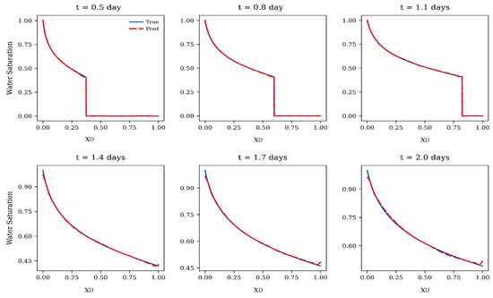
Figure 7. Comparison of TL-FNO predictions (red dashed lines) with analytical Buckley–Leverett at M = 2 to the target regime of M = 5.

While the baseline FNO fails to generalize when the mobility ratio shifts to M = 5, over-estimate the water saturations, the TL-FNO successfully adapts with only limited target data. By reusing spectral features from the source regime and fine-tuning selected layers, the TL-FNO provides accurate front propagation, demonstrating a substantial improvement in both accuracy and data efficiency. Table 5 demonstrates that the TL-FNO achieves excellent extrapolation performance when transferring from the training regime ($M=2$) to the target regime ($M=5$).

Table 5. Extrapolation Accuracy of TL-FNO for $M=5$.

Time (Days)	R2	MAE	MSE
0.5	0.999	7.0 × 10−3	7.4 × 10−6
0.8	0.999	1.4 × 10−3	3.6 × 10−6
1.1	0.999	1.0 × 10−3	3.2 × 10−6
1.4	0.999	1.0 × 10−3	5.8 × 10−6
1.7	0.998	2.0 × 10−3	1.5 × 10−5
2.0	0.998	3.4 × 10−3	3.2 × 10−5

Across all time snapshots, the model maintains exceptionally high accuracy, with $R^2$ values exceeding 0.998 and MSE and MAE remaining several orders of magnitude smaller than those of the baseline FNO. Errors increase slightly at later times, reflecting the greater difficulty of capturing sharper displacement fronts as the saturation evolves, but remain very small overall. These results indicate that transfer learning effectively leverages knowledge from the source regime and enables robust adaptation to new mobility ratios with limited target data, significantly outperforming the baseline model in both accuracy and stability.

3.4. Physics-Informed Neural Operator Performance

While transfer learning improves the adaptability of FNOs across parameter regimes, it remains fundamentally data-driven and dependent on representative training samples. To further enhance extrapolative reliability, we incorporate the B-L equation directly into the operator-learning framework. In addition, to capture the flow characteristics of subsurface reservoirs under different mobility ratios, the mobility ratio M was explicitly incorporated into the FNO training dataset. Using the same formation and fluid parameters listed in Table 1, M was varied between 1 and 10. Consequently, the input tensor takes the form (2048, 8192, 3), where the three channels correspond to water saturation, spatial sampling, and mobility ratio. An FNO was trained to predict the saturation profile at a later time (t = 2.0 days) from the profile at an earlier time (t = 0.5 day) across the range of mobility ratios. Figure 8 compares the FNO predictions with analytical B-L solutions for different interpolated values of M. The results demonstrate that the model interpolates well across the mobility-ratio spectrum, with the predicted saturation fronts closely matching the analytical benchmarks.

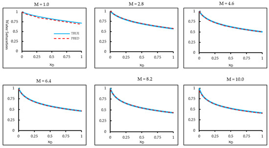
Figure 8. Comparison of baseline FNO predictions with the analytical Buckley–Leverett solution across the interpolation range of mobility ratios. The analytical solution is shown as a blue solid line, and the corresponding FNO prediction is shown as a red dashed line. Within the training regime, the baseline FNO accurately reconstructs the saturation profiles and captures the displacement front.

Table 6 summarizes the interpolation performance of the FNO when predicting B-L saturation profiles at mobility ratios lying between the training samples. Across all tested values of $M$, the model achieves excellent agreement with the analytical solutions, with $R^2$ consistently above 0.98 and MSE and MAE remaining on the order of ${10}^{-4}$~${10}^{-2}$. The accuracy is highest for intermediate values (e.g., $M=2.8$~6.4), where both MAE and MSE fall below ${10}^{-2}$, reflecting smooth interpolation within the learned parameter manifold. Even at the edges of the interpolation range ($M=1.0$ and $M=10.0$), the model maintains strong performance, demonstrating robust parametric generalization. These results indicate that the baseline FNO effectively captures the mobility-ratio dependence of fractional flow dynamics and provides reliable predictions for intermediate parameter values. However, its reliability diminishes when applied outside the training domain, motivating the use of physics-informed and transfer-learning strategies to improve extrapolation.

Table 6. FNO Interpolation Accuracy Across Mobility Ratios $M$.

Mobility Ratio $\mathit{M}$	R2	MAE	MSE
1.0	0.981	7.3 × 10−3	1.2 × 10−4
2.8	0.993	8.1 × 10−3	8.1 × 10−5
4.6	0.996	7.5 × 10−3	5.9 × 10−5
6.4	0.995	8.3 × 10−3	7.7 × 10−5
8.2	0.995	8.1 × 10−3	8.5 × 10−5
10.0	0.992	1.0 × 10−2	1.4 × 10−4

Figure 9 compares the analytical B-L solution with model predictions for extrapolation to mobility ratio M = 15, a regime beyond the training range of [1, 10]. The comparison (Figure 9a) reveals that the baseline FNO captures the overall decreasing trend of water saturation with distance but exhibits a systematic underestimation across the entire domain. The predicted saturation front is displaced downward, reflecting the model’s inability to replicate the stronger instability and sharper displacement front associated with the higher mobility ratio. This discrepancy indicates that the trained operator, although effective within its original parameter regime, struggles to generalize to more extreme flow contrasts.

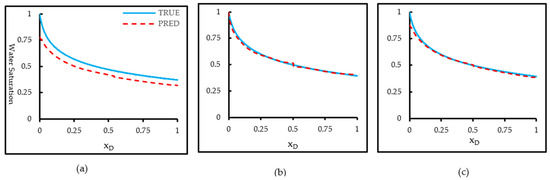
Figure 9. Extrapolation performance of Fourier Neural Operator models for a mobility ratio of $M=15$, which lies outside the training range. (a) Baseline FNO prediction (red dashed line) compared with the analytical Buckley–Leverett solution (blue solid line); (b) Physics-Informed FNO (PI-FNO) prediction, showing improved shock sharpness and front alignment; (c) Transfer-Learned FNO (TL-FNO) prediction adapted from a source model trained on $M\in [1, 10]$ and fine-tuned using limited $M=15$ samples.

The PI-FNO shown in Figure 9b demonstrates significant improvement. By embedding PDE residuals and enforcing initial and boundary conditions, the model closely reproduces the analytical saturation distribution. The close agreement between the two curves demonstrates that embedding physical constraints into the learning framework significantly enhances generalization beyond the training domain. The physics-constrained model accurately captures both the nonlinear curvature near the inlet and the smooth saturation decline along the spatial domain, preserving the underlying flux-saturation relationship dictated by the governing equation. The TL-FNO in Figure 9c also enhances extrapolation performance compared with the baseline. Through fine-tuning a pretrained FNO from the M = 10 regime using 300 target samples at M = 15, the TL-FNO achieves reduced error and better alignment with the analytical solution, effectively capturing the nonlinear saturation profile throughout most of the domain. The strong correspondence indicates that knowledge adaptation from pre-trained models enhances the learning of transport dynamics under new mobility conditions. Nevertheless, slight deviations near the inlet suggest residual bias in reproducing the steep saturation gradient, likely due to local variations not fully represented in the source domain. The overall accuracy remains slightly below that of PI-FNO.

Table 7 summarizes the extrapolation performance of the Baseline FNO, PI-FNO, and TL-FNO at a mobility ratio of M = 15 and confirms the trends observed in Figure 9, providing quantitative support for the visual comparison of extrapolation performance among the three models.

Table 7. Comparative extrapolation performance of Baseline FNO, TL-FNO, and PI-FNO at M = 15.

Model	R2	MAE	MSE
Baseline FNO	0.785	1.12 × 10−1	1.36 × 10−2
TL-FNO	0.978	3.72 × 10−2	2.05 × 10−3
PI-FNO	0.983	3.12 × 10−2	1.02 × 10−3

In summary, PI-FNO delivers the most accurate and physically consistent extrapolation, while TL-FNO offers strong performance with higher data efficiency. Together, these approaches effectively mitigate the limitations of the baseline FNO in shock-dominated regimes beyond the training domain.

From a practical perspective, the proposed Physics-Informed and Transfer-Learned Fourier Neural Operators (PI-FNO and TL-FNO) provide a general framework that can be seamlessly integrated into industrial reservoir simulation workflows. Once trained, these operator-based surrogates can rapidly predict spatiotemporal saturation distributions for new boundary, initial, or parameter conditions, achieving orders-of-magnitude speedup compared with conventional simulators. The PI-FNO enhances physical consistency through PDE-based regularization, whereas the TL-FNO enables efficient adaptation to new reservoir conditions with limited data, making both models well suited for large-scale optimization, history matching, and uncertainty quantification. For real-world applications such as heterogeneous reservoirs and multidimensional geometries, the corresponding data and governing PDEs must be incorporated to ensure physical representativeness and model fidelity. Although model training introduces an upfront computational cost, it is performed offline and requires only moderate hardware resources. Overall, the proposed method is general, scalable, and complementary to existing simulators, providing a practical pathway toward real-time, data-efficient modeling of multiphase flow in complex reservoir systems.

If the B-L equation were extended to include heterogeneous porous media, compressibility, or capillary effects, the extrapolative performance of both PI-FNO and TL-FNO would likely depend on the accuracy with which these additional physical mechanisms are represented in the governing equations and training data. The PI-FNO could potentially maintain physical consistency by incorporating extended PDE residuals and additional terms in the loss function, but its performance might degrade if the underlying physics or constitutive relationships are incomplete or highly nonlinear. In heterogeneous or multidimensional reservoirs, the spatial variability in permeability and saturation fronts introduces stronger gradients and localized discontinuities, which may challenge the current one-dimensional formulation. Consequently, the PI-FNO may exhibit reduced accuracy or slower convergence in such cases, while the TL-FNO could alleviate part of this degradation by leveraging pretrained operators from similar physical regimes and adapting them to complex domains with limited fine-scale data. Future work will therefore focus on extending the methodology to heterogeneous and multidimensional systems through multi-fidelity learning, adaptive loss weighting, and hierarchical domain decomposition, thereby enhancing the robustness, generality, and scalability of operator learning for realistic reservoir applications.

4. Conclusions

This study examined the extrapolative performance of FNOs applied to the B-L problem, a benchmark problem for shock-dominated multiphase flow. While the baseline FNO demonstrated excellent interpolation accuracy within the training regime, it failed to generalize reliably to longer time horizons and shifted mobility ratios, producing inaccurate predicted saturation fronts. To address these shortcomings, two complementary strategies were introduced. The PI-FNO embedded PDE residuals, initial and boundary conditions, and entropy constraints directly into the training loss, yielding sharper displacement fronts and improved physical consistency. The TL-FNO leveraged pretrained spectral representations and fine-tuning with limited target data, enabling efficient adaptation to new regimes. Comparative analysis confirmed that both approaches reduced extrapolation error significantly, with PI-FNO providing the most robust performance across regimes.

These findings underscore the importance of integrating physics constraints and knowledge transfer in operator learning, offering a pathway toward reliable, data-efficient surrogates for multiphase flow modeling in porous media. Future work will extend these strategies to heterogeneous reservoirs, multidimensional geometries, and more complex recovery processes such as chemical flooding and gas injection.

References

- Buckley, S.E.; Leverett, M.C. Mechanism of fluid displacement in sands. Trans. AIME 1942, 146, 107–116. [Google Scholar] [CrossRef]
- Dake, L.P. Fundamentals of Reservoir Engineering; Elsevier: Amsterdam, The Netherlands, 1978. [Google Scholar]
- Qiao, Y.; Hatzignatiou, D.G. Analytical Solution for Chemical Fluid Injection into Linear Heterogeneous Porous Media Based on the Method of Characteristics. Chem. Eng. Sci. 2023, 282, 119337. [Google Scholar] [CrossRef]
- Khan, M.Y.; Mandal, A. Improvement of Buckley-Leverett Equation and Its Solution for Gas Displacement with Viscous Fingering and Gravity Effects at Constant Pressure for Inclined Stratified Heterogeneous Reservoir. Fuel 2021, 285, 119172. [Google Scholar] [CrossRef]
- Johns, R.T.; Orr, F.M. Miscible gas displacement of multicomponent oils. In Proceedings of the SPE Annual Technical Conference and Exhibition, Dallas, TX, USA, 22–25 October 1995. [Google Scholar] [CrossRef]
- Lake, L.W.; Johns, R.; Rossen, W.R.; Pope, G.A. Fundamentals of Enhanced Oil Recovery; Society of Petroleum Engineers: Richardson, TX, USA, 2014. [Google Scholar]
- Welge, H.J. A simplified method for computing oil recovery by gas or water drive. Trans. AIME 1952, 195, 91–98. [Google Scholar] [CrossRef]
- Chen, Z.; Huan, G.; Ma, Y. Computational Methods for Multiphase Flows in Porous Media; Society for Industrial and Applied Mathematics: Philadelphia, PA, USA, 2006. [Google Scholar] [CrossRef]
- Raissi, M.; Perdikaris, P.; Karniadakis, G.E. Physics-informed neural networks: A deep learning framework for solving forward and inverse problems involving nonlinear PDEs. J. Comput. Phys. 2019, 378, 686–707. [Google Scholar] [CrossRef]
- Diab, W.; Chaabi, O.; Zhang, W.; Arif, M.; Alkobaisi, S.; Al Kobaisi, M. Data-free and data-efficient physics-informed neural network approaches to solve the Buckley–Leverett problem. Energies 2022, 15, 7864. [Google Scholar] [CrossRef]
- Fraces, C.G.; Papaioannou, A.; Tchelepi, H.A. Physics-informed deep learning for transport in porous media: Buckley-Leverett problem. arXiv 2020, arXiv:2001.05172. [Google Scholar]
- Zhang, F.; Nghiem, L.; Chen, Z. A novel approach to solve hyperbolic Buckley–Leverett equation by using a transformer-based physics-informed neural network. Geoenergy Sci. Eng. 2024, 236, 212711. [Google Scholar] [CrossRef]
- Almajid, M.M.; Abu-Al-Saud, B. Prediction of porous media fluid flow using physics-informed neural networks: Application to Buckley–Leverett. J. Pet. Sci. Eng. 2022, 208, 109205. [Google Scholar] [CrossRef]
- Ma, X.; Li, C.; Zhan, J.; Zhuang, Y. Physics-informed generative adversarial network solution to Buckley–Leverett equation. Mathematics 2024, 12, 3833. [Google Scholar] [CrossRef]
- Li, Z.; Kovachki, N.; Azizzadenesheli, K.; Liu, B.; Bhattacharya, K.; Stuart, A.M.; Anandkumar, A. Fourier neural operator for parametric partial differential equations. In Proceedings of the International Conference on Learning Representations (ICLR), Virtual Event, Austria, 3–7 May 2021. [Google Scholar] [CrossRef]
- Alpak, F.O.; Vamaraju, J.; Jennings, J.W.; Pawar, S.; Devarakota, P.; Hohl, D. Augmenting deep residual surrogates with Fourier neural operators for rapid two-phase flow and transport simulations. SPE J. 2023, 28, 2982–3003. [Google Scholar] [CrossRef]
- Zhao, X.; Chen, X.; Gong, Z.; Zhou, W.; Yao, W.; Zhang, Y. RecFNO: A resolution-invariant flow and heat field reconstruction method from sparse observations via Fourier neural operator. Int. J. Therm. Sci. 2024, 195, 108619. [Google Scholar] [CrossRef]
- Pathak, J.; Subramanian, S.; Harrington, P.; Raja, S.; Chattopadhyda, A.; Mardani, M. FourCastNet: A global data-driven highresolution weather model using adaptive Fourier neural operators. arXiv 2022, arXiv:2202.11214. [Google Scholar]
- Li, Z.; Peng, W.; Yuan, Z.; Wang, J. Fourier neural operator approach to large eddy simulation of three-dimensional turbulence. Theor. Appl. Mech. Lett. 2022, 12, 100389. [Google Scholar] [CrossRef]
- Tang, H.; Kong, Q.; Morris, J.P. Multi-fidelity Fourier neural operator for fast modeling of large-scale geological carbon storage. J. Hydrol. 2024, 629, 130641. [Google Scholar] [CrossRef]
- Song, C.; Wang, Y. High-frequency wavefield extrapolation using the Fourier neural operator. J. Geophys. Eng. 2022, 19, 269–282. [Google Scholar] [CrossRef]
- Azzizadenesheli, K.; Kovachki, N.B.; Li, Z.; Liu-Schiaffini, M.; Kossaifi, J.; Anandkumar, A. Neural Operators for Accelerating Scientific Simulations and Design. arXiv 2023, arXiv:2309.15325. [Google Scholar] [CrossRef]
- Mao, Z.; Zhang, H.; Jiao, A.; Karniadakis, G.E.; Lu, L. Reliable extrapolation of deep neural operators informed by physics or sparse observations. J. Comput. Phys. 2023, 491, 112401. [Google Scholar] [CrossRef]
- Li, Z.; Zheng, H.; Kovachki, N.; Jin, D.; Chen, H.; Liu, B.; Azizzadenesheli, K.; Anandkumar, A. Physics-Informed Neural Operator for Learning Partial Differential Equations. arXiv 2021, arXiv:2111.03794. [Google Scholar] [CrossRef]
- Eshaghi, M.S.; Anitescu, C.; Thombre, M.; Wang, Y.; Zhuang, X.; Rabczuk, T. Variational Physics-Informed Neural Operator (VINO) for Solving Partial Differential Equations. Comput. Methods Appl. Mech. Eng. 2025, 437, 117785. [Google Scholar] [CrossRef]
- Xu, J.; Li, Z.; Zhang, Y.; Liu, Q. Transfer Learning of Neural Operators for Partial Differential Equations (λ-FNO). PLoS ONE 2025, 20, e0321154. [Google Scholar] [CrossRef] [PubMed]
- Wang, Y.; Zhang, H.; Lai, C.-T.; Hu, X. Transfer Learning Fourier Neural Operator for Solving Parametric Frequency-Domain Wave Equations. IEEE Trans. Geosci. Remote Sens. 2024, 62, 5923211. [Google Scholar] [CrossRef]
- Ma, X.; Zhong, R.; Zhan, J.; Zhou, D. Enhancing subsurface multiphase flow simulation with Fourier neural operator. Heliyon 2024, 10, 18. [Google Scholar] [CrossRef]
- Lyu, Y.; Zhao, X.; Gong, Z.; Kang, X.; Yao, W. Multi-fidelity Prediction of Fluid Flow Based on Transfer Learning Using Fourier Neural Operator. Phys. Fluids 2023, 35, 077118. [Google Scholar] [CrossRef]
- Corey, A.T.; Rathjens, C.H.; Henderson, J.H.; Wyllie, M.R.J. Three-phase relative permeability. J. Petrol. Technol. 1956, 8, 63–65. [Google Scholar] [CrossRef]
- Wu, S. Multiphase Fluid Flow in Porous and Fractured Reservoirs; Gulf Professional Publishing: Houston, TX, USA, 2015. [Google Scholar]
- Karniadakis, G.E.; Kevrekidis, I.G.; Lu, L.; Perdikaris, P.; Wang, S.; Yang, L. Physics-informed machine learning. Nat. Rev. Phys. 2021, 3, 422–440. [Google Scholar] [CrossRef]
- Hu, E.J.; Shen, Y.; Wallis, P.; Allen-Zhu, Z.; Li, Y.; Wang, S.; Wang, L.; Chen, W. LoRA: Low-Rank Adaptation of Large Language Models. arXiv 2021, arXiv:2106.09685. [Google Scholar]
Disclaimer/Publisher’s Note: The statements, opinions and data contained in all publications are solely those of the individual author(s) and contributor(s) and not of MDPI and/or the editor(s). MDPI and/or the editor(s) disclaim responsibility for any injury to people or property resulting from any ideas, methods, instructions or products referred to in the content. |
© 2025 by the authors. Licensee MDPI, Basel, Switzerland. This article is an open access article distributed under the terms and conditions of the Creative Commons Attribution (CC BY) license (https://creativecommons.org/licenses/by/4.0/).