Abstract
This work develops and systematically evaluates a physics-informed neural network (PINN) solver for the fully coupled, time-dependent Muskat–Leverett system with capillarity modeled in the pressure equation. A single shallow–wide multilayer perceptron jointly predicts wetting pressure and water saturation; physical capillary pressure regularizes the saturation front, while a small numerical diffusion term in the saturation residual acts as a training stabilizer rather than a shock-capturing device. To guarantee admissible states in stiff regimes, we introduce a saturation soft-clamping head enforcing and activate it selectively for stiff mobility ratios. Using IMPES solutions as reference, we perform a sensitivity study over network depth and width, interior collocation and boundary data density, mobility ratio, and injection pressure. Shallow-wide networks (10 layers × 50 neurons) consistently outperform deeper architectures, and increasing interior collocation points from 5000 to 50,000 reduces mean saturation error by about half, whereas additional boundary data have a much weaker effect. Accuracy is highest at an intermediate mobility ratio and improves monotonically with higher injection pressure, which sharpens yet better conditions the front. Across all regimes, pressure trains easily while saturation determines model selection, and the PINN serves as a physics-consistent surrogate for what-if studies in two-phase porous-media flow.
1. Introduction
The simultaneous flow of two immiscible fluids in a porous medium is a foundational problem in subsurface engineering. It governs the success of industrial applications ranging from waterflooding and enhanced oil recovery (EOR) [1] to the long-term security of geological sequestration [2]. The classical framework for this problem was established by a series of seminal mid-century contributions.
The field was first codified by Muskat (1937), who provided the comprehensive mathematical treatment for fluid flow in porous media [3], followed by Buckley and Leverett’s (1942) formulation of the 1D fractional flow model [4]. While these models successfully predicted the formation of sharp saturation shock, later solvable via Welge’s graphical method [5], they rely on a hyperbolic, inviscid assumption that is fundamentally reductionist. By neglecting capillary pressure, these classical frameworks fail to capture the diffusive physics critical to modern applications. In scenarios such as sequestration or EOR, the mathematically convenient sharp shock is a physical impossibility; the actual front is smeared by capillary forces, rendering the pure hyperbolic solution insufficient for accurate plume tracking.
This 1D Buckley–Leverett framework, however, ignored two critical physical phenomena. The first was the effect of capillarity, which Leverett (1941) had quantified with his dimensionless J-function, providing a method to scale the static capillary pressure curve based on rock and fluid properties [6]. The second was the stability of the displacement front itself. Saffman and Taylor demonstrated that when a less viscous fluid displaces a more viscous one (an unfavorable mobility ratio, ), the front is unstable and degenerates into “viscous fingers” [7]. This body of work, synthesized in texts by Homsy [8], Bear [9], Helmig [10], and Blunt [11], shows the competing, complex physics of advection, diffusion (capillarity), and instability.
In modern applications, modeling capillarity is not optional. For storage, capillary heterogeneity is a dominant control on plume migration, residual trapping, and ultimate storage security [2]. For EOR, wettability and capillary-driven spontaneous imbibition are key levers for maximizing recovery [1].
However, the classical static capillary pressure model () is itself an idealization. A more rigorous thermodynamic framework introduced by Hassanizadeh and Gray established that capillary pressure is also a function of non-equilibrium effects, specifically the rate of saturation change [12]. This dynamic capillarity concept was later validated by dynamic pore-network models [13].
The mathematical consequence of incorporating dynamic capillarity is profound. As demonstrated by Spayd and Shearer, it transforms the governing equation from a first-order hyperbolic PDE into a third-order, non-linear pseudo-parabolic PDE [14]. This shift in mathematical character exposes the limitations of standard numerical schemes. The introduction of dispersive, undercompressive shock structures makes the equation notoriously stiff. Consequently, traditional finite volume or difference schemes often require computationally expensive stabilizing techniques to resolve these non-monotonic profiles without introducing spurious oscillations.
Given this complexity, industrial simulators typically solve the fully coupled pressure–saturation system, often referred to as the Muskat–Leverett system [15,16]. Formulations such as the global pressure approach [17] were developed to stabilize the elliptic pressure solve. The most common solution algorithms are IMPES (IMplicit Pressure, Explicit Saturation) and its variants [18].
These classical schemes, however, suffer from significant numerical drawbacks. Standard IMPES solvers do not inherently guarantee local mass conservation or respect the physical bounds [19]. While physics-preserving schemes have been developed to enforce these constraints [20], they achieve stability only at the cost of algorithmic complexity and increased computational overhead. The necessity for these rigorous, iterative corrections highlights the fragility of discrete mesh-based solvers in stiff regimes, motivating the search for alternative methods.
Physics-Informed Neural Networks (PINNs) have emerged as a powerful, mesh-free alternative for solving such PDEs [21]. However, they face a fundamental, well-documented failure mode when applied to the very equations that define multiphase flow: hyperbolic conservation laws.
A foundational critique by Fuks and Tchelepi demonstrated that vanilla PINNs, which encode the PDE as a soft penalty in the loss function, are inadequate for solving the non-linear hyperbolic Buckley–Leverett equation [22]. The trained networks fail to converge to the correct solution and are incapable of representing the sharp saturation shock [23].
This failure is not a simple training issue; it is a fundamental limitation. The consensus in the literature points to two root causes:
Spectral Bias: Deep neural networks are inherently biased toward learning low-frequency (smooth) functions first. They struggle to learn the high-frequency components that constitute a sharp discontinuity [24].
Continuity Assumption: The network’s architecture, built from smooth activation functions, is infinitely differentiable. It is therefore mathematically ill-suited to approximating a discontinuous function [25].
This core failure also manifests as “propagation failure,” where the network fails to correctly propagate the initial conditions through time [26].
An intense research effort has focused on overcoming this failure, primarily through artificial regularization. Fuks and Tchelepi (2020) proposed adding Artificial Viscosity (AV) to transform the hyperbolic PDE into a parabolic one [22], a concept refined by Coutinho et al. using adaptive localized viscosity [27]. However, these methods represent a methodological compromise. They rely on introducing a non-physical numerical diffusion term solely to stabilize the training process, effectively smearing the shock based on heuristics rather than physics. Similarly, hybrid approaches that inject analytical Welge solutions [28] are limited to simplified 1D cases where analytical solutions exist. Critically, this reliance on artificial viscosity overlooks a fundamental physical reality: the reservoir already possesses a natural regularization mechanism, physical capillary pressure, which is intrinsic to the governing equations yet frequently neglected in PINN formulations to simplify the training architecture.
The physical phenomenon of capillary pressure, when included in the governing equations, intrinsically introduces a second-order spatial derivative that naturally smooths the shock front. It therefore acts as a physical regularization mechanism, replacing the need for non-physical numerical aids. To our knowledge, systematic studies that treat physical capillarity in the coupled Muskat–Leverett PINN as the primary regularizer for transient two-phase flow are scarce.
Alternative strategies have focused on increasing architectural complexity. Domain decomposition methods (cPINN/XPINN) [29,30] break the problem into subdomains, while sequence-based models—such as Transformers (PINNsFormer) [26,31] and attention-enhanced LSTMs [32]—explicitly model temporal dependencies to overcome propagation failure. Similarly, convolutional encoder–decoder architectures like physics-informed U-Nets have been proposed to accelerate flow simulations [33]. The search for more powerful and efficient solvers for multiphase flow has pushed researchers to explore paradigms beyond classical deep learning, leading to novel proposals such as quantum-classical hybrid architectures designed specifically for the Muskat–Leverett equations [34]. While effective, these approaches increase the computational graph size and training complexity. They effectively treat the symptom (spectral bias) by engineering more complex networks, rather than addressing the root cause: the formulation of the PDE itself.
To address physical admissibility, such as boundary conditions or state bounds, hard constraint methods have been developed. These range from complex optimization schemes like the augmented Lagrangian method (hPINNs) [35] to simpler, direct architectural changes. This directly addresses the tendency of PINNs to overshoot or undershoot near steep gradients [36].
This review reveals a clear and critical gap. The vast majority of the PINN literature on two-phase flow has focused intensely on solving the 1D, saturation-only, inviscid Buckley–Leverett “toy problem”. While this is a vital benchmark for shock-capturing, it avoids the complexities of a real-world system.
- The vast majority of PINN literature focuses on the decoupled, saturation-only Buckley–Leverett equation. This represents a critical oversimplification for heterogeneous media. These models ignore the critical bidirectional coupling where saturation changes alter mobility by treating velocity as a fixed parameter, which in turn dynamically redistributes the pressure field. While a limited number of studies have attempted to solve the fully coupled, time-dependent Muskat–Leverett system [37,38], they remain the exception. In our previous work, we have modeled both pressure and saturation [39]; however, the formulation simplified the pressure equation by omitting the capillary potential. Consequently, a fully coupled PINN framework for transient Muskat–Leverett flow that rigorously incorporates capillarity in the pressure equation and systematically exploits this physical capillarity as the primary regularizer, rather than relying on non-physical artificial viscosity in the saturation equation, remains absent.
- A large portion of existing PINN shock-capturing approaches introduce an explicit artificial viscosity (AV) term directly into the Buckley–Leverett equation to smooth the shock and stabilize training. While effective for the inviscid BL benchmark, these AV-PINNs modify the governing physics by prescribing a numerical viscosity that controls the front width. In contrast, our formulation relies on the physical capillary pressure term in the coupled Muskat–Leverett system as the primary regularization mechanism. A small numerical diffusion is used only as a training stabilizer in the saturation residual (not as a shock-capturing mechanism), while the physically correct capillary term dictates the front structure. While Chakraborty et al. [40] successfully modeled a coupled system with capillary heterogeneity, their analysis was restricted to steady-state conditions, thereby sidestepping the numerical instability of transient shock propagation entirely.
- The physical constraint of saturation is a known failure point for classical [41] and PINN solvers [42], yet a direct, hard-constraint clamping approach is not standard practice in existing two-phase PINN models. To address this, we introduce a saturation clamping mechanism as a hard constraint, which is selectively activated to guarantee physical admissibility in stiff regimes (e.g., high mobility ratios).
- Finally, most PINN studies demonstrate a single solution [40]. They fail to deliver on the promise of a true surrogate model by quantifying performance and sensitivity across a range of engineering parameters, such as mobility ratio () and injection pressure [43].
This study directly addresses these four gaps. We present a PINN framework for the fully coupled, time-dependent pressure–saturation (Muskat–Leverett) system that retains physical capillarity in the pressure equation and systematically leverages this term as the primary regularization mechanism for training, reducing reliance on non-physical artificial viscosity in the saturation equation. Our model employs a shared multi-output network to co-predict pressure () and saturation (), and we introduce a saturation clamping method as a hard constraint to guarantee physical admissibility for stiff . Finally, we validate this framework as a surrogate by mapping performance across mobility ratio () and injection pressure, with the aim of showing its value as a physics-consistent reservoir simulation, which can be evaluated at arbitrary space–time points once trained.
2. Mathematical Model
2.1. Governing Equations
To achieve a more physically realistic description of immiscible displacement, the Muskat–Leverett (ML) model extends the Buckley–Leverett formulation by incorporating the effects of capillary pressure, [17]. Capillary pressure is the pressure difference across the interface between two immiscible fluids in the pores of the medium, arising from interfacial tension. It is a function of saturation, , and is defined as the pressure in the non-wetting phase minus the pressure in the wetting phase:
The inclusion of this term fundamentally changes the physics and the mathematical structure of the problem. The pressure gradients for the individual phases are no longer equal. Substituting the capillary pressure relation into Darcy’s law for the non-wetting phase yields:
where and are the phase mobilities, [9,44].
The system of equations is derived from the conservation of mass for each phase, assuming incompressibility. The divergence of the total velocity must be zero [45,46]:
Substituting the Darcy-level expressions for the phase velocities gives
This can be rearranged into a wetting-phase pressure equation, which is elliptic in nature for a given saturation field. Here, the primary variable is the wetting phase pressure, :
Letting be the total mobility, the pressure equation becomes
The second term in the divergence operator, , represents the capillary-driven flux. Physically, this term acts as a non-linear diffusion mechanism, driving the wetting phase from regions of high saturation to low saturation.
In the context of the displacement front, this capillary diffusion opposes the steepening effect of advection. While the hyperbolic Buckley–Leverett model (where ) predicts the formation of a mathematically discontinuous shock, the inclusion of this capillary term smears the front into a steep but continuous transition zone with a finite width.
This physical characteristic is particularly advantageous for Physics-Informed Neural Networks. Since neural networks approximate functions using continuous compositions of smooth activation functions, they struggle to represent true discontinuities (the Gibbs phenomenon). By explicitly modeling the capillary term, we replace the discontinuity with a smooth, physically regularized front that is inherently more learnable for the network, reducing the need for artificial shock-capturing techniques.
With the pressure field defined by this elliptic balance, the temporal evolution of the system is governed by the conservation of mass for the wetting phase. Unlike the pressure equation, which represents an instantaneous equilibrium of forces, the following equation dictates the transient transport of the fluid:
Substituting Darcy’s law for the wetting phase velocity, , yields the final saturation transport equation. Here, the coupling becomes explicit: the saturation evolution is driven by the pressure gradient , which in turn has been shaped by the capillary forces in Equation (7). The final saturation transport equation is given as
The Muskat–Leverett model is therefore a coupled system of two non-linear PDEs. The pressure depends on the saturation through the mobility terms, while the temporal evolution of is driven by the pressure gradient . The capillary term in the pressure equation introduces a second-order spatial derivative of saturation, effectively adding a diffusion-like term to the system. This term regularizes the sharp shock front of the BL solution, transforming it into a continuous, albeit steep, transition zone.
2.2. Constitutive Relationships
The governing equations are closed by specifying the constitutive relationships that describe the fluid and rock properties. For this study, the following functional forms are employed:
Relative permeabilities—quadratic forms are maintained for consistency with the BL model:
Capillary pressure, which is a non-linear, empirical function of saturation, is employed [16]:
The parameter scales the magnitude of the capillary forces. As , the diffusive effects vanish, and the system behavior approaches that of the Buckley–Leverett model. While dynamic capillarity can be important, we adopt a static law here and attribute dispersion in transients primarily to the pressure equation’s capillary term; extending to dynamic forms is future work.
Non-Dimensionalization and Reference Scales
To generalize the analysis, the governing equations are cast into a dimensionless form.
Let be the domain length and the imposed pressure drop. We define the dimensionless variables:
A characteristic Darcy velocity based on the wetting viscosity is .
Choosing the time scale to absorb porosity,
which yields the dimensionless ML system (dropping the subscript ):
where , , and .
In this formulation, plays the role of an artificial diffusion coefficient that regularizes the saturation front; in all experiments it is prescribed based on the target physical regime and held fixed during training unless otherwise stated.
This non-dimensionalization simplifies the system by scaling the absolute permeability and wetting-phase viscosity scale to unity. Consequently, the porosity is absorbed into the time scale, and the fluid properties are consolidated into a single parameter, the viscosity ratio, which governs the non-wetting phase mobility . The artificial diffusion is dimensionless.
Results reported versus () are comparable across cases; physical time is recovered by . Thus, increasing speeds up the physical evolution even if the dimensionless dynamics versus () look similar.
With , , and the porosity factor is absorbed into time, so in the dimensionless ML system, we set .
3. Methodology
3.1. Physics-Informed Neural Network (PINN) Framework for the Muskat Leverett Problem
While prior work has applied PINNs to two-phase flow [39], the inclusion of the capillary pressure term in the pressure equation introduces a second-order spatial derivative of saturation, significantly increasing the complexity of the PDE system and the corresponding loss functional.
3.1.1. Network Architecture
A single Multi-Layer Perceptron (MLP) is employed to co-approximate both the pressure and saturation fields. The network architecture takes the spatio-temporal coordinates as input. The output layer is modified to have two neurons, yielding a two-dimensional output vector:
This shared-parameter architecture allows the network to learn the intricate, non-linear coupling between the pressure and saturation fields implicitly during training. The activation function is retained for the hidden layers. The network’s output for saturation is trained unconstrained initially. However, to ensure training stability in stiff regimes (e.g., high mobility ratios), we selectively enable a bounded output head for via a sigmoid transformation with a small buffer, , as detailed in the mobility ratio sensitivity analysis. This constraint is enabled a priori for the mobility-ratio cases , where preliminary experiments showed occasional excursions of outside or overshoots near the front. For the moderate cases and , the saturation output remains unconstrained because the network already respects the physical bounds without clamping.
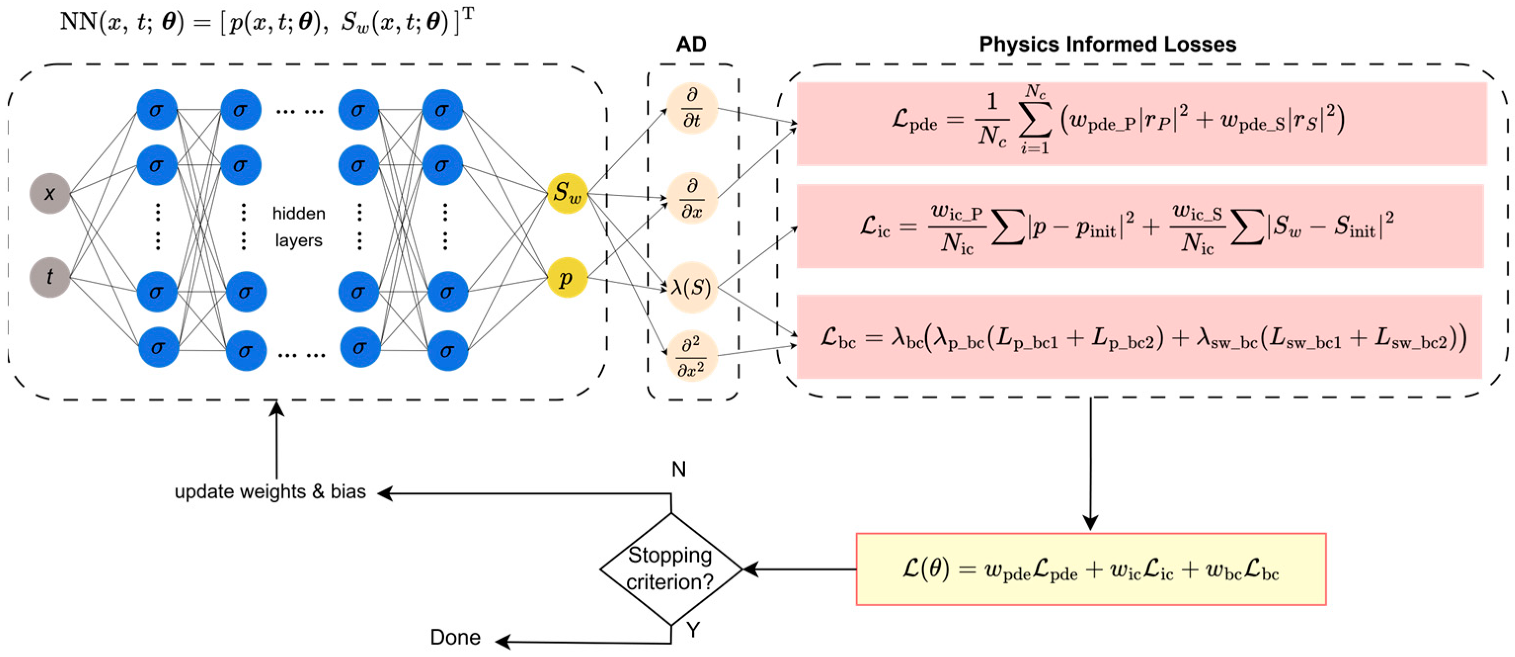
The PINN framework is adapted to solve this coupled system by predicting both fields simultaneously from a single network. A schematic of this architecture and its corresponding loss functional is shown in Figure 1.
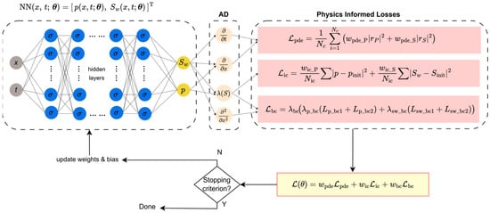
Figure 1.
PINN architecture for the coupled Muskat–Leverett problem. The network takes (x, t) as input and has two outputs for the simultaneous prediction of saturation () and pressure (). The loss function is constructed from the residuals of both the pressure and saturation PDEs, in addition to the initial and boundary condition data.
3.1.2. Loss Functional
The loss functional for the ML model is significantly more complex, as it must enforce the physics and data constraints for both the pressure and saturation equations. The PINN is trained to minimize the residuals of the two coupled governing equations.
While the physical capillarity term provides the primary regularization by ensuring the saturation front is a continuous function, the dynamics can still be very “stiff,” leading to steep gradients in the loss landscape. To enhance numerical stability, we include a small fixed numerical diffusion term only in the saturation residual to smooth the optimization landscape; capillarity governs the physical front and is tuned conservatively. This term acts as a numerical regularizer that aids the optimizer’s convergence, while the magnitude and shape of the physical front are primarily dictated by the capillary pressure model. The value of is a hyperparameter determined during the calibration study.
The pressure equation residual () enforces the elliptic pressure balance (total velocity divergence-free) including the capillary term.
where is the total mobility.
The saturation equation residual () residual enforces the mass conservation of the wetting phase.
The total PDE loss, , is the sum of the mean squared errors of these two residuals over the collocation points:
The data loss term enforces the initial and boundary conditions for both fields.
Initial Condition (IC) Loss () enforces the initial pressure and saturation at .
Boundary Condition (BC) Loss () enforces a combination of Dirichlet and Neumann boundary conditions.
Fixed pressure (Dirichlet) values are imposed at both the inlet () and outlet ().
For saturation, a Dirichlet condition is applied at the inlet (), and a homogeneous Neumann condition (), representing no diffusive flux, is applied at the outlet ().
The total BC loss is .
The complete loss functional is a weighted sum of the PDE, IC, and BC components, reflecting the multi-objective nature of the optimization problem.
For this study, all loss weights () are fixed to 1.0 to provide a balanced contribution from each physical and data constraint. This choice is supported by two factors. First, our component-wise convergence analysis demonstrates that the pressure and saturation residuals naturally decay at similar rates and magnitudes, indicating that the coupled system does not suffer from severe scale imbalances that would require normalization. Second, our previous systematic investigation of loss weighting strategies for the same unified pressure–saturation PINN architecture in the Buckley–Leverett setting [39], where extensive sweeps over global and saturation-specific weights showed that strongly non-uniform weights can degrade overall solution quality and that configurations close to unit weights offer robust performance. In the present work, we therefore focus the sensitivity analysis on (i) model architecture, (ii) data density, and (iii) physical parameters (mobility ratio and injection pressure), while keeping the scalar weights fixed.
We did not employ gradient normalization or NTK-based adaptive weighting in this study; integrating such schemes with the capillary-augmented coupled Muskat–Leverett system is left to future work.
3.1.3. Data Generation and Partitioning
Unlike traditional supervised learning, the dataset for this PINN framework consists of coordinate points sampled from the spatiotemporal domain . We employed Latin Hypercube Sampling (LHS) [47] to ensure space-filling coverage of the domain, avoiding the clustering issues often seen with simple random sampling.
A fixed number of points (ranging from 100 to 300 per boundary) were sampled specifically for the initial and boundary conditions. These are entirely allocated to the training loss term and .
A set of collocation points were generated via LHS. To ensure the network learns generalized physics rather than overfitting to specific coordinate locations, we applied a random 80/20 split:
- -
- 80% (Training): Used to minimize the PDE residual loss .
- -
- 20% (Validation): Used to monitor the generalization of the PDE residual during training, ensuring the solution remains physically valid at unseen points within the domain.
Post-training evaluation was performed on a completely independent, dense, uniform grid of size . The PINN predictions on this grid were compared against the high-fidelity numerical reference solution to compute the relative L2 error metrics reported in the results.
3.2. Numerical Experiments
3.2.1. Hyperparameter Calibration
To establish a baseline model for subsequent analyses, a systematic hyperparameter calibration was performed. The process involved a grid search over the primary architectural and regularization parameters to identify the configuration that minimizes prediction error against a high-fidelity numerical reference. The search space is defined by combinations of the following hyperparameters:
- -
- Network Depth (): {10, 20, 30} hidden layers.
- -
- Network Width (): {20, 30, 50} neurons per layer.
- -
- Artificial Diffusion Coefficient (): {0.001, 0.0035, 0.00535}. The values of are chosen to span a range from weak to moderate regularization of the saturation front while remaining consistent with the underlying physical regime and numerical resolution. We also tested a variant in which is treated as a trainable scalar parameter optimized jointly with the network weights; however, the learned values remained close to the baseline settings and did not yield consistent improvements in accuracy. To avoid adding complexity without clear benefit, we therefore keep fixed in the results reported here and leave more general adaptive parameterizations to future work.
Mobility Ratio () was fixed at 3.0 and all weights () are set to 1.0. This experiment used (per condition) and , which is in line with common PINN baselines that employ data points and collocation points for 1D time-dependent PDEs [21,48,49].
Next, the collocation points and the data points for the initial and boundary conditions are generated using Latin Hypercube Sampling (LHS) [47,50]. This quasi-random sampling technique ensures a more uniform, space-filling distribution of points across the spatio-temporal domain compared to simple random sampling, leading to more efficient training.
Finally, a two-stage optimization procedure is employed to train the network parameters .
Stage 1 (Adam Optimizer)—The training process begins with the Adam optimizer (1000 Adam epochs (learning rate ), a first-order gradient-based algorithm well-suited for navigating the complex and often non-convex loss landscapes of neural networks [51].
Stage 2 (L-BFGS Optimizer)—After a set number of Adam iterations, the optimization switches to the Limited-memory Broyden–Fletcher–Goldfarb–Shanno (L-BFGS) algorithm. L-BFGS is a quasi-Newton method that can achieve faster convergence and higher precision once the solution is near a local minimum. Here, we use up to 20,000 L-BFGS iterations [52]. We use this two-stage approach because Adam’s stochastic adaptivity helps escape poor minima and quickly reach a good basin, while the quasi-Newton L-BFGS exploits curvature information to overcome the PINN loss’s ill-conditioning and drive fast, high-precision convergence [53,54,55].
The performance of each configuration is measured by the relative L2 error [56] against the high-fidelity numerical solution described in the previous section.
In our case, the relative L2 error for a variable (pressure or water saturation ) at an evaluation time is computed on a uniform spatial grid by taking the Euclidean norm of the pointwise difference between the high-fidelity reference (the numerical solution) and the PINN prediction, normalized by the reference norm. Concretely, we sample both fields on the same nodes (interpolating the reference to the evaluation grid when necessary) and evaluate:
with a small () added to the denominator in code to avoid division by zero. Unless otherwise stated, we summarize performance by the mean of over a representative set of evaluation times, , reported separately for () and (); these scores determine the baseline configuration.
3.2.2. Sensitivity to Training Data
The second objective is to analyze the dependence of the PINN solution accuracy on the quantity of training data. This is investigated using a full factorial experimental design over the number of data points () and collocation points (). The model architecture and other hyperparameters are kept fixed to the optimal baseline configuration identified in the previous task. The configuration for this experiment is 10 layers and 50 neurons, with 0.0035 and 3.0, identified as suitable from the previous analysis. The model is trained and evaluated for every combination of the following parameters, resulting in 9 experimental runs.
- Data Points (): {100, 200, 300}. Each run uses points for the initial condition, points for the inlet boundary condition, and for the outlet, resulting in a total of 3 × data points.
- Collocation Points (): {5000, 15,000, 50,000}
3.2.3. Sensitivity to Fluid Mobility Ratio
For the coupled ML system, increasing the mobility ratio amplifies the convective forces relative to the capillary diffusion, leading to a much steeper saturation front. This “stiff” behavior poses a significant challenge for PINN training, often causing convergence issues or inaccurate solutions. To address this, a key modification was introduced to the baseline PINN framework: an architectural constraint on the saturation output.
The experiment utilizes the optimal architecture identified from the data regime study, 10 layers, 50 neurons, = 0.0035, 200 and 50,000 .
Preliminary experiments revealed that training was unstable for mobility ratios at the extremes of the tested range ( and ) and showed smaller, but still noticeable, overshoots at . To improve training stability and prevent the network from predicting physically implausible saturation values (e.g., ), especially near the steep or strongly diffusive front, we activate the soft clamping mechanism only for . For and The head remains unconstrained, as these runs do not exhibit violations of the physical bounds. Instead of an unbounded output, a soft clamping mechanism was implemented using the sigmoid function:
where is the raw output from the network’s final linear layer, is the sigmoid function, and is a small constant (. This transformation strictly constrains the predicted saturation to the range (), avoiding the problematic endpoints and where the capillary pressure function has singularities. The pressure output remains unbounded.
Using this modified framework, the PINN is trained and evaluated for each mobility ratio in the set with clamping applied only to the cases. Crucially, this clamping prevents the network from predicting non-physical negative saturation values (). Since the capillary pressure function (Equation (11)) contains a term proportional to , any excursion near or below zero results in a singularity. This would generate exploding gradients in the PDE residual destabilizing the optimization. The soft constraint therefore acts as a necessary numerical safety guard to ensure well-posed gradients throughout the training process. This approach allows for a detailed assessment of the PINN’s performance on increasingly convective-dominant problems.
3.2.4. Sensitivity to Injection Pressure
The final objective is to assess the sensitivity of the Muskat–Leverett PINN model to the injection pressure, a key operational parameter that directly influences the overall pressure gradient and the speed of the fluid displacement. This analysis is performed exclusively on the ML model, as pressure is not an explicit variable in the Buckley–Leverett formulation.
The PINN model is trained on a dimensionless version of the governing equations where the pressure field is scaled to the range The physical injection pressure and production pressure are mapped to dimensionless values of 1 and 0, respectively. The key parameter that links the physical and dimensionless worlds is the capillary pressure prefactor, The dimensionless prefactor, , used in the PINN’s loss function is derived from the physical prefactor, , and the total pressure drop across the domain,
In this study, is held constant at and the production pressure is fixed at 0.10.
The experiment utilizes the PINN configuration established in Section 3.2.2 for the mobility ratio study, including the architectural modification for saturation clamping.
The PINN is trained and evaluated for a set of five different physical injection pressures. For each case, a corresponding numerical simulation is also run with the same physical parameters to serve as a reference solution. The experimental cases are defined as seen in Table 1.

Table 1.
Experimental cases for physical and dimensionless values for .
3.3. Computing Environment and Training Setup
All experiments were run on a single workstation equipped with an NVIDIA RTX 5080 (16 GB VRAM). The implementation uses PyTorch 2.10.0.dev20251016+cu128, Python 3.12.3, NumPy 2.3.3 for modeling, and Matplotlib 3.10.7 for visualizations. All runs are single-GPU and use the same sampling strategy and loss construction specified in Section 3.1 and Section 3.2. Reproducibility is supported by fixing the random seed, saving model checkpoints and logs, and retaining the exact dependency versions listed above.
4. Results
To provide a benchmark for all experiments, high-fidelity reference solutions were generated using a numerical solver based on an Implicit Pressure, Explicit Saturation (IMPES) scheme. The solution to the Muskat–Leverett system is characterized by a diffusive saturation front. The spatial domain was discretized into uniform grid cells (). Temporal evolution was managed via a fixed time-stepping strategy with a dimensionless step size of (1,000,000 steps for ), which strictly satisfies the Courant–Friedrichs–Lewy (CFL) stability condition for the explicit saturation update. The pressure equation was solved using an iterative Gauss–Seidel scheme with a convergence tolerance of , while the saturation was updated using a first-order upwind scheme to ensure monotonic shock propagation. The capillary pressure term was treated explicitly, lagging to the saturation values from the previous time step.
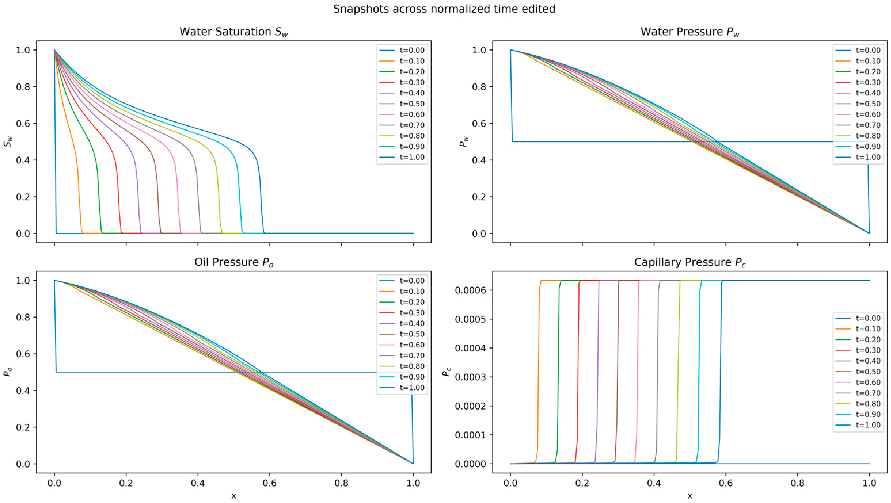
Figure 2 displays a representative solution for the baseline case of , showing the spatio-temporal evolution of the pressure and saturation fields. It is crucial to note that for each experimental case presented in the subsequent sections, a unique numerical reference was generated with the identical set of physical parameters (e.g., mobility ratio, injection pressure). All PINN predictions are compared against their corresponding ground truth solution.
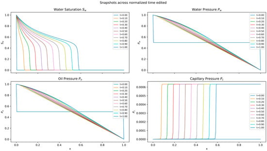
Figure 2.
Numerical solution of the Muskat–Leverett system for . The panels show the evolution of (top-left) water saturation, which exhibits a diffusive front; (top-right) water pressure; (bottom-left) oil pressure; and (bottom-right) capillary pressure.
4.1. Hyperparameter Calibration: Establishing a Baseline Model
The first phase of the investigation focused on identifying an optimal PINN architecture through a systematic hyperparameter search. The objective was to find a configuration capable of accurately resolving the complex interplay between convective transport and capillary diffusion inherent in the Muskat–Leverett model. The results of this grid search are detailed in Table 2 for the top 15 models ranked by mean L2 ().

Table 2.
Results for hyperparameter search across diffusion, layers and neurons (.
While Table 2 reports only global relative L2 errors, it is also important to understand how the discrepancy between the PINN and IMPES solutions is distributed in space and time. Figure 3 summarizes this error structure for the baseline case . Figure 3a shows the space–time map of the absolute saturation error, revealing that the dominant discrepancies are confined to a narrow neighborhood of the moving saturation front, with both the injected and displaced regions remaining within . Figure 3b displays the corresponding pressure error, which is uniformly small throughout the domain and thus corroborates the very low reported in Table 2. To resolve the leading-edge behavior more clearly, Figure 3c plots spatial profiles of the saturation error at , and . These slices show that the global scores are dominated by localized peaks at the front rather than by large errors in the bulk, providing a more intuitive picture of the model’s strengths and limitations.
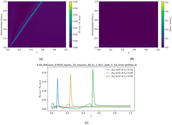
Figure 3.
Spatial and temporal structure of the PINN–IMPES discrepancy for the baseline case . (a) Space–time map of the absolute saturation error . The error field is highly localized: the largest discrepancies occur along the moving saturation front, whereas both the injected and displaced regions remain within over the entire simulation. (b) Corresponding space–time map of the absolute pressure error for , which remains uniformly small across the domain, consistent with the low values reported in Table 2. (c) Spatial slices of the saturation error at three representative times . In all cases, the error exhibits a narrow, front-centered peak with a width comparable to the physical transition zone, while background errors away from the front remain small. These profiles confirm that the global L2 metrics in Table 2, Table 3, Table 4 and Table 5 are dominated by localized discrepancies at the advancing front rather than by a broad bias in the bulk solution.
Although increasing provides additional numerical smoothing in the saturation equation, Table 2 shows that larger values consistently lead to higher saturation error. This implicitly demonstrates that when physical capillarity (from the pressure equation) is allowed to dominate, the solution matches the ground truth more closely than when additional numerical diffusion is imposed. This internal trend serves as a scientifically meaningful alternative to AV-PINN comparisons, because it isolates the role of numerical vs. physical regularization while keeping the governing PDE identical.
Analysis of the marginal effects reveals a distinct and critical trend regarding network depth. Increasing the network depth from 10 to 20, and further to 30, leads to a severe degradation in performance, with the mean L2 error for saturation increasing by orders of magnitude. The massive error bars for the 30-layer networks indicate severe training instability. This suggests that for this coupled, second-order PDE system, very deep architectures are difficult to optimize and prone to issues like vanishing/exploding gradients. Consequently, a shallower network of 10 layers demonstrates markedly superior performance and stability for this problem.
Conversely, network width shows an opposing trend, where increasing the number of neurons from 20 to 50 per layer leads to a significant improvement in accuracy. The configurations with 30 and 50 neurons achieve significantly lower L2 errors and much smaller variance compared to the 20-neuron networks. This indicates that a wider network is necessary to provide the capacity to approximate both the saturation and pressure fields simultaneously.
The choice of is critical for the coupled ML system. The marginal analysis in Figure 4 shows that yields the most stable results on average, significantly reducing the extreme variance seen with lower values. This highlights that substantial regularization is generally required to stabilize the training of this sensitive system. The marginal effects of the hyperparameters on the average L2 error for saturation (L2 ()) are shown in Figure 4. (Note: The error scale for some configurations was very large, indicating training failure; these outliers can skew the visual representation but highlight the sensitivity of the problem.)
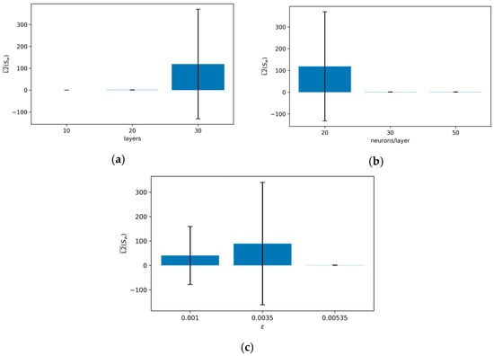
Figure 4.
Marginal effects of layers, neurons, and on the mean L2 error for saturation (L2 ()) in the ML model. (a) Number of layers vs. L2 (); (b) number of neurons per layer vs. L2 (); (c) vs. L2 ().
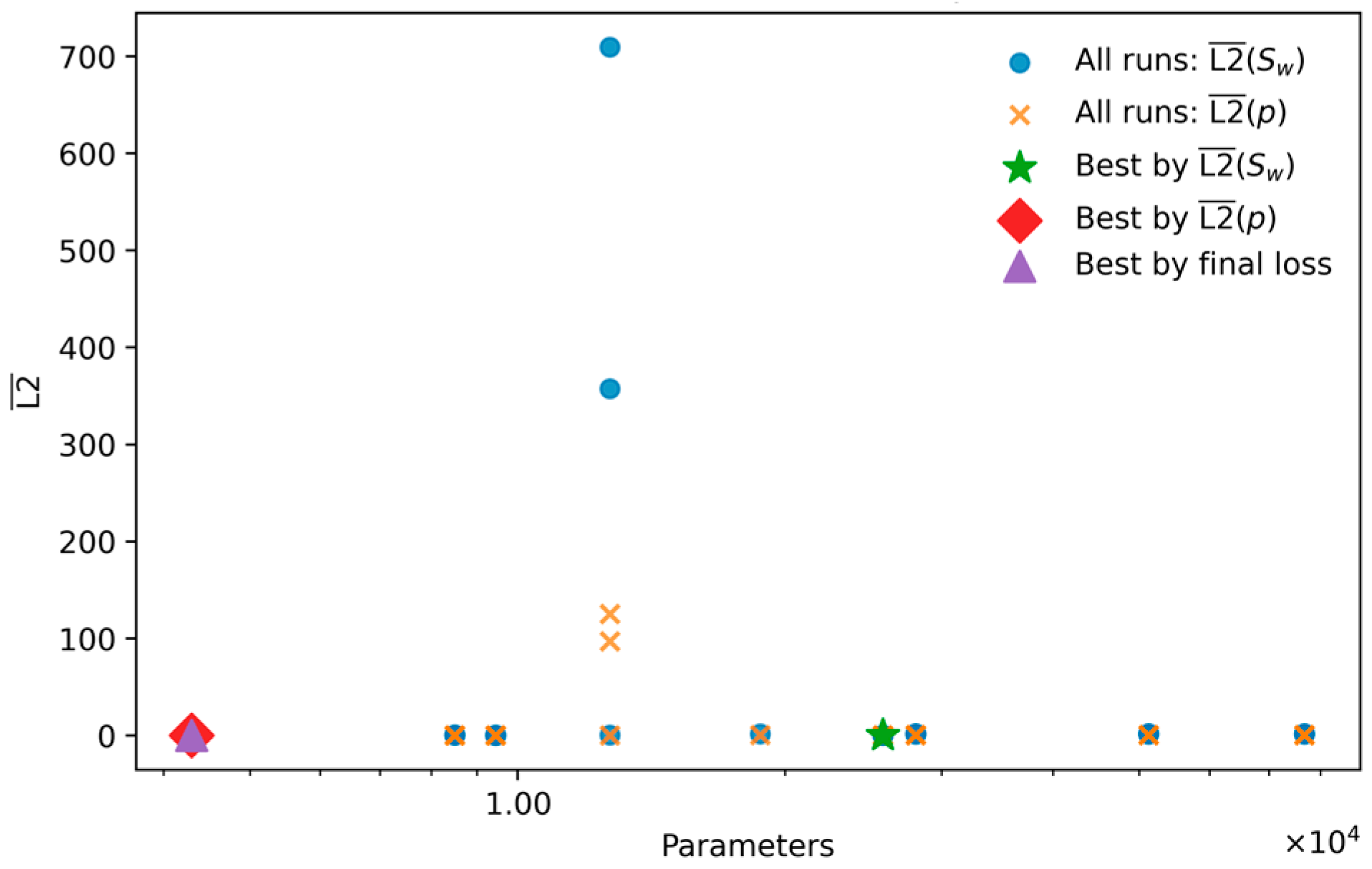
While the marginal analysis provides general guidance, selecting the optimal model requires examining the performance of individual configurations, as visualized in the scatter plot of Figure 5. This revealed a critical performance trade-off: the configuration yielding the highest saturation accuracy (L2 () = ) for a 10-layer, 50-neuron network with was not the same as the one that achieved the best pressure accuracy ( for a 10-layer, 20-neuron network, ), as per Table 2.
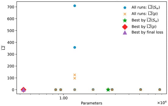
Figure 5.
L2 error of saturation and pressure vs. number of trainable parameters.
This indicates that while higher regularization () ensures general stability, a slightly lower value () allowed the best-performing architecture to achieve a more accurate representation of the challenging saturation front. Given that capturing the saturation profile is the primary difficulty in two-phase flow modeling, the model that minimizes L2 () is the most suitable choice. Therefore, the 10-layer, 50-neuron network with is selected as the baseline architecture for the subsequent sensitivity analyses of the Muskat–Leverett model.
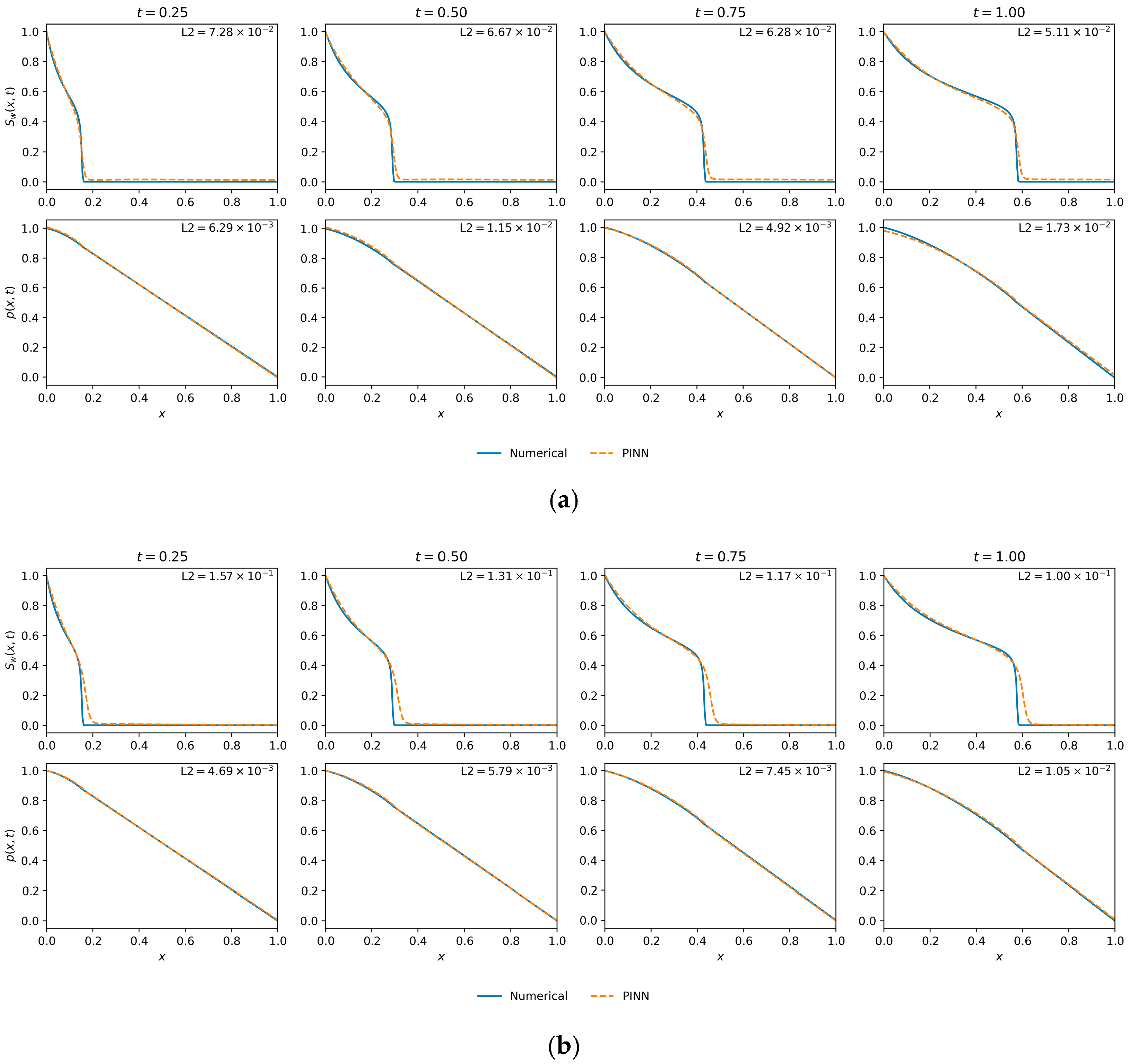
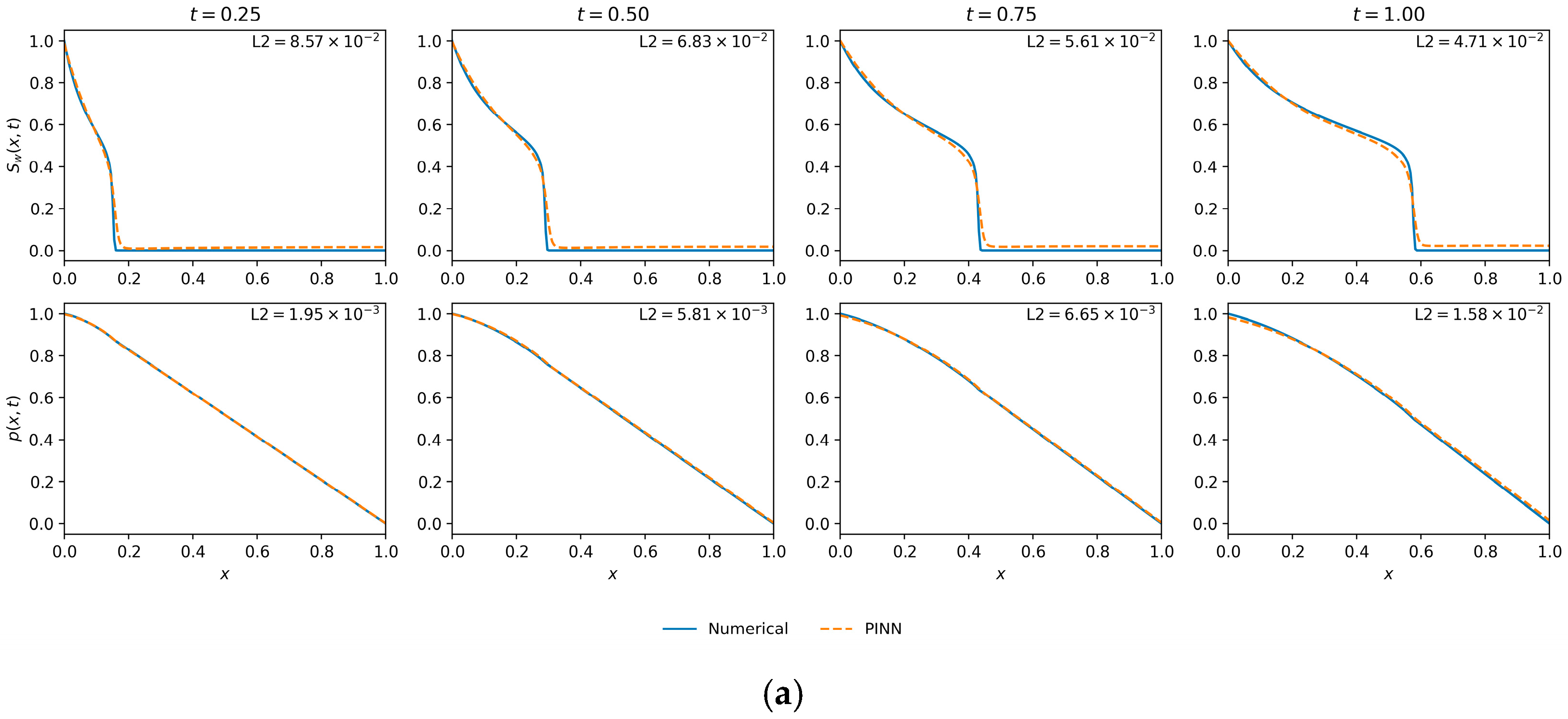
Figure 6 provides a visual comparison of the performance of the two top-performing models. The Best by L2 () model (top row) shows high fidelity with the numerical solution for both saturation and pressure. The diffusive saturation front, characteristic of capillary action, is accurately captured at all time steps. The pressure profile is also predicted with high fidelity.
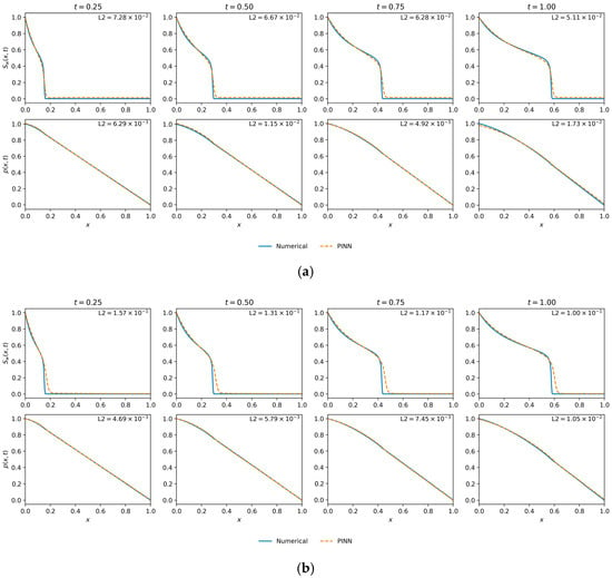
Figure 6.
Saturation and pressure profile comparisons for two optimal models from the hyperparameter search. (a) The model achieving the lowest saturation error (Best by L2()—(10-layer, 50 neurons, ε = 0.0035)). (b) The model achieving the lowest pressure error (Best by L2(p)—(10-layer, 20 neurons, ε = 0.00535)), which also yielded the lowest final training loss. Impact of data density on solution accuracy.
The Best by L2 (p) and Final Loss model (bottom row), while accurately predicting the pressure, shows a noticeable discrepancy in the saturation profile. The front is slightly smeared and phase-shifted compared to the numerical reference, leading to a higher saturation error.
This comparison confirms that the 10-layer, 50-neuron network provides the best overall physical representation and is the appropriate choice for the baseline model.
Having established a baseline architecture, this analysis investigates the PINN’s sensitivity to the density of training points (10 layers, 50 neurons, ). The experiment systematically varied the number of data points enforcing the boundary and initial conditions () and the number of collocation points enforcing the governing physics within the domain (). The complete results of this factorial experiment are presented in Table 3.

Table 3.
Results for sensitivity analysis across different data types and quantities (, .
To assess the statistical reliability of these findings, we conducted a multi-seed variability analysis for representative configurations. This revealed a critical link between data density and algorithmic robustness. For sparse collocation regimes (), the optimization proved highly sensitive to network initialization, with certain random seeds leading to premature stagnation or divergence. In contrast, the dense configuration () demonstrated significantly improved stability. Across converged runs, the dense model yielded a low standard deviation in saturation error ), which is an order of magnitude smaller than the mean error itself. This confirms that increasing the density of physics enforcement does not merely lower the approximation error, as shown in Table 3, but also convexifies the optimization landscape, making the training process far more reproducible and less dependent on a lucky initialization.
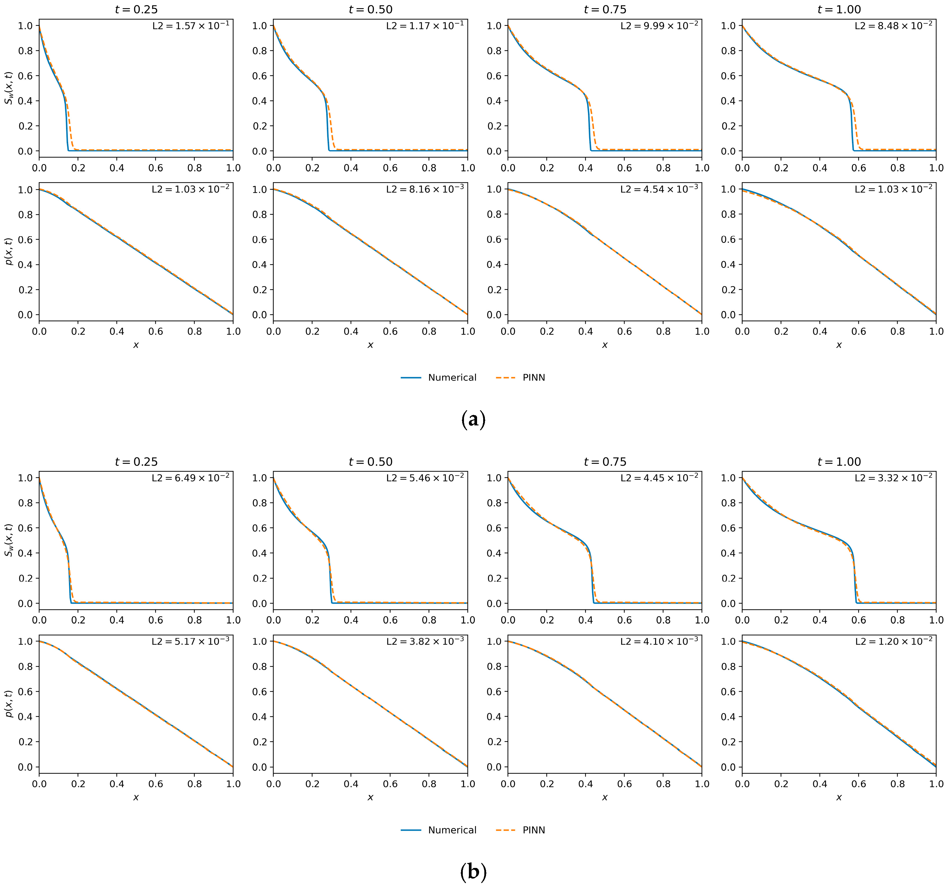
The analysis reveals that the number of collocation points, is the single most dominant factor influencing solution accuracy. As shown in the marginal effects plot in Figure 7, increasing from 5000 to 50,000 results in a substantial and monotonic decrease in the mean saturation error (L2 ()), reducing it from approximately 0.16 to 0.07. This dramatic improvement underscores the necessity of densely enforcing the PDE residuals throughout the spatio-temporal domain. For a complex, coupled system involving second-order derivatives and non-linearities like the Muskat–Leverett model, a strong enforcement of the underlying physics is paramount.
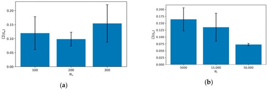
Figure 7.
Sensitivity of L2 () to initial data points () and collocation points (). (a) L2(); (b) vs. L2().
In stark contrast, the number of boundary data points, , exerted a much weaker and less consistent influence on performance. The marginal plot for in Figure 7 shows large error variance and a non-monotonic trend, suggesting that once a sufficient number of boundary constraints are provided, the solution accuracy becomes primarily limited by the enforcement of the internal physics rather than the boundary conditions themselves.
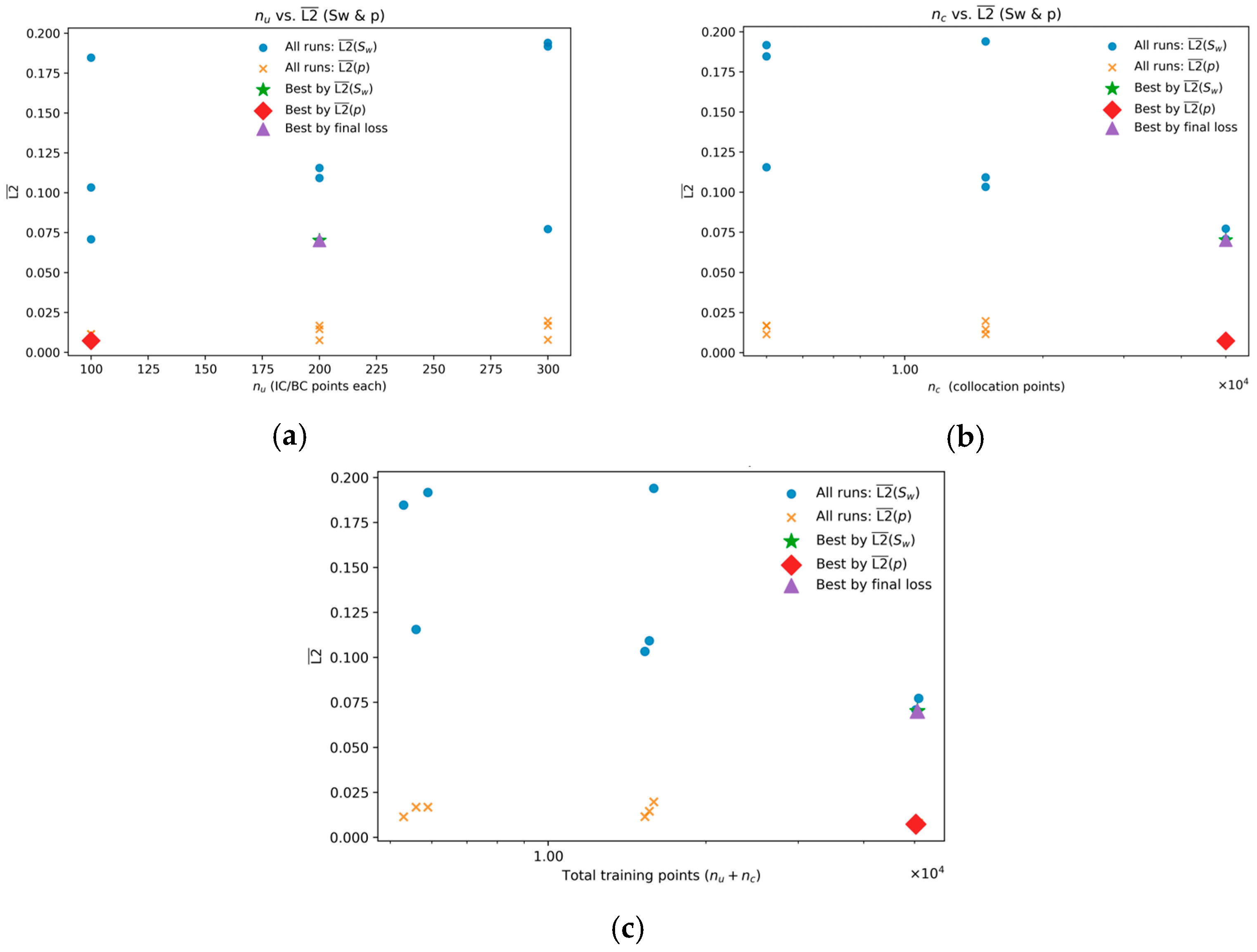
These aggregate trends are confirmed by the performance of individual experimental runs, detailed in Table 3 and visualized in the scatter plots of Figure 8. The plots clearly show that while the pressure error (L2 (p)) remains low and relatively stable across all configurations, the saturation error (L2 ()) is highly sensitive to . Notably, all the most accurate models are clustered in the high- region (), with the best results achieved at . The optimal configuration, which achieved the lowest saturation error (L2() ), was found with and . As indicated by the markers in Figure 8 and the data in Table 3, this configuration also yielded the lowest final training loss, making it the unambiguous best-performing model.
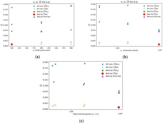
Figure 8.
Variation of the mean L2 error in saturation and pressure with (a) the number of initial/boundary-condition points L2 () (b) the number of collocation points L2 (), and (c) their total () L2 (). Each marker represents an independent run; symbols denote best models ranked by L2 (), L2 (p), and final loss.
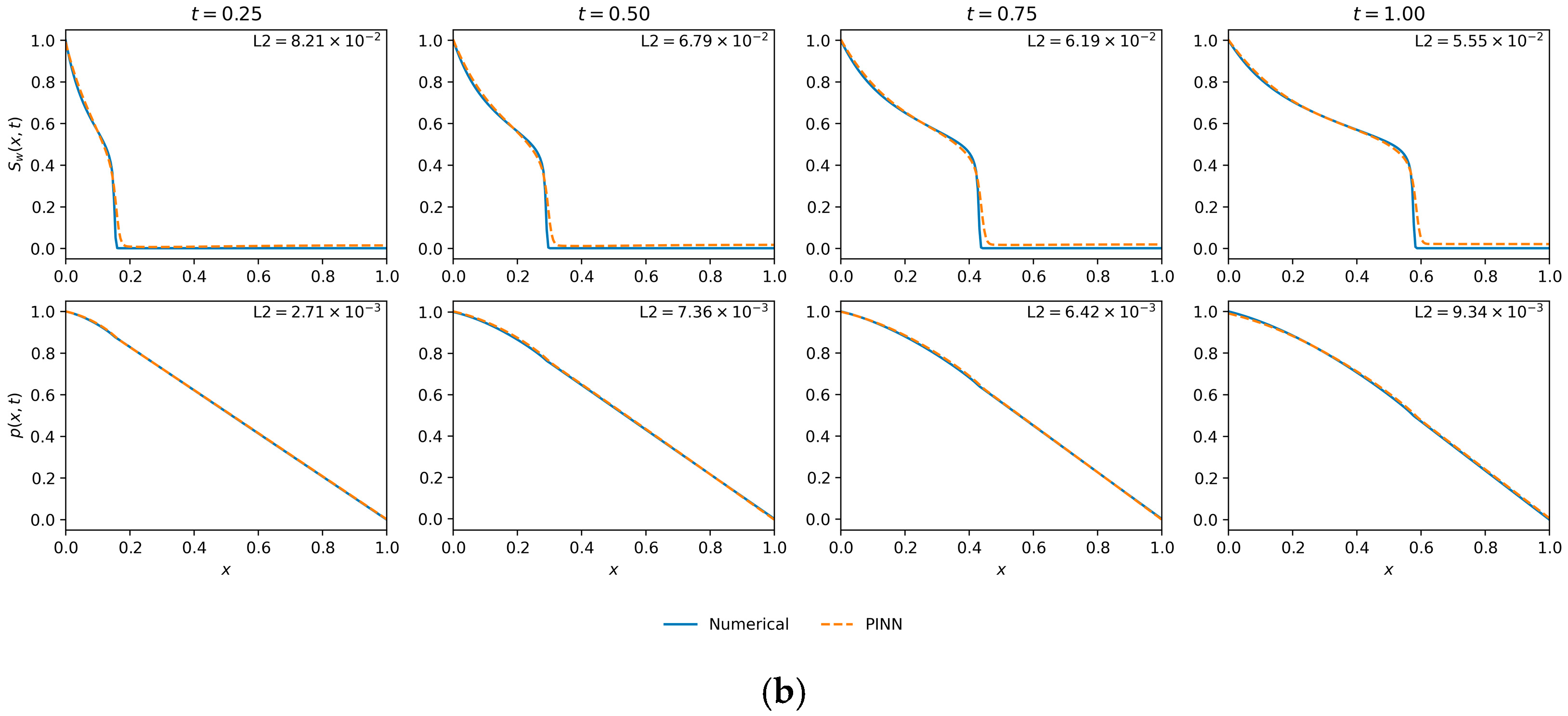
The quantitative findings are substantiated by the qualitative results presented in Figure 9. This figure showcases the spatio-temporal profiles from the premier configuration identified in this study ( = 200, = 50,000), which, according to Table 3, achieved both the lowest saturation error (L2 () = ) and the lowest final training loss. There is strong visual correspondence between the PINN solution and the numerical ground truth; the model captures the diffusive front and pressure field accurately across all representative time steps. This confirms that a high density of collocation points enables the PINN to function as a high-fidelity solver for the Muskat–Leverett system. Therefore, this optimal data configuration (, 50,000) will be used as the baseline for the subsequent parametric sensitivity studies.
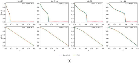
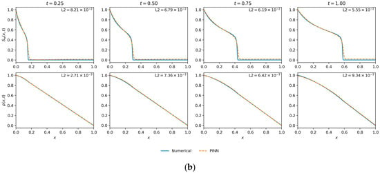
Figure 9.
Saturation and pressure profile comparisons from the data density analysis. (a) The optimal configuration, which achieved both the lowest saturation error (L2 ()) and the lowest final loss ( ). (b) The configuration that resulted in the lowest pressure error (L2 (p) ( )).
4.2. Sensitivity to Fluid Mobility Ratio
To assess the validity of the PINN framework, its performance was evaluated across a range of fluid mobility ratios (M), a parameter that fundamentally governs the system’s physical behavior by controlling the balance between viscous (convective) and capillary (diffusive) forces. The specialized PINN architecture with saturation clamping, as described in the methodology, was employed to ensure training stability across all cases. The comprehensive results of this parametric study are detailed in Table 4.

Table 4.
Results for sensitivity analysis across different values of M (.
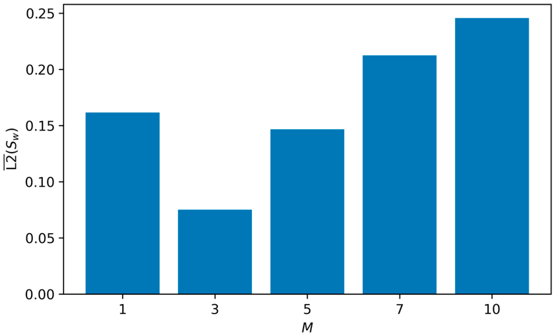
The results reveal a distinct, non-monotonic relationship between the mobility ratio and the prediction accuracy for saturation, as summarized in the marginal effects plot in Figure 10. The PINN achieves its highest accuracy at , yielding the lowest mean L2 error for saturation (L2() = ) and pressure (). Performance degrades for both lower and higher values of , indicating that the model’s efficacy is dependent on the specific physical regime.
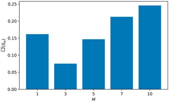
Figure 10.
Influence of M on the mean L2 error for saturation (L2 ()).
A critical observation is the asymmetry in performance between the two fields. The pressure error (L2 (p)) is an order of magnitude lower than the saturation error and remains relatively stable across all mobility ratios. The key insight is that the pressure field is smooth and lacks the sharp advective front, making it uniformly easy for the PINN to learn, which is why we utilize the saturation error L2 () as the dominant and most meaningful metric for assessing the model’s ability to handle the challenging physics of each regime.
At the intermediate mobility ratio of , the system exhibits a healthy balance between convective and capillary forces. This creates a well-defined yet smooth saturation front that is highly amenable to approximation by the PINN, resulting in high accuracy.
With a low mobility ratio of , capillary forces are relatively dominant, leading to a broad, highly diffusive saturation front. The model struggles to perfectly capture the full spatial extent of this dispersion, resulting in a higher error ().
As increases (), the system becomes progressively convection-dominated. This results in a much steeper, “stiff” saturation front that approaches a shock-like profile. This stiffness poses a significant challenge for approximation by the inherently smooth neural network, causing a noticeable phase lag and smearing of the front, which worsens as increases to 10 ().
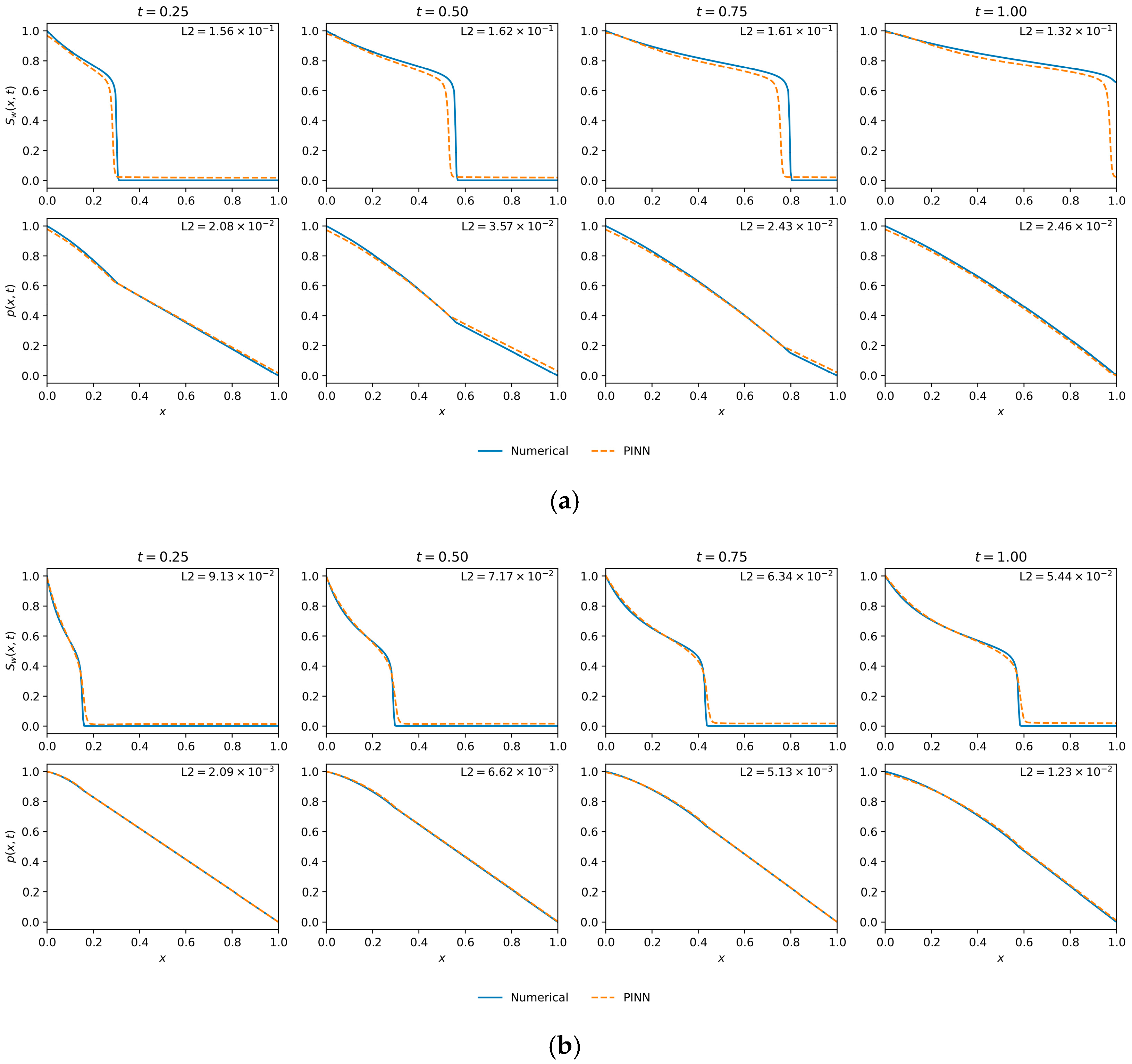
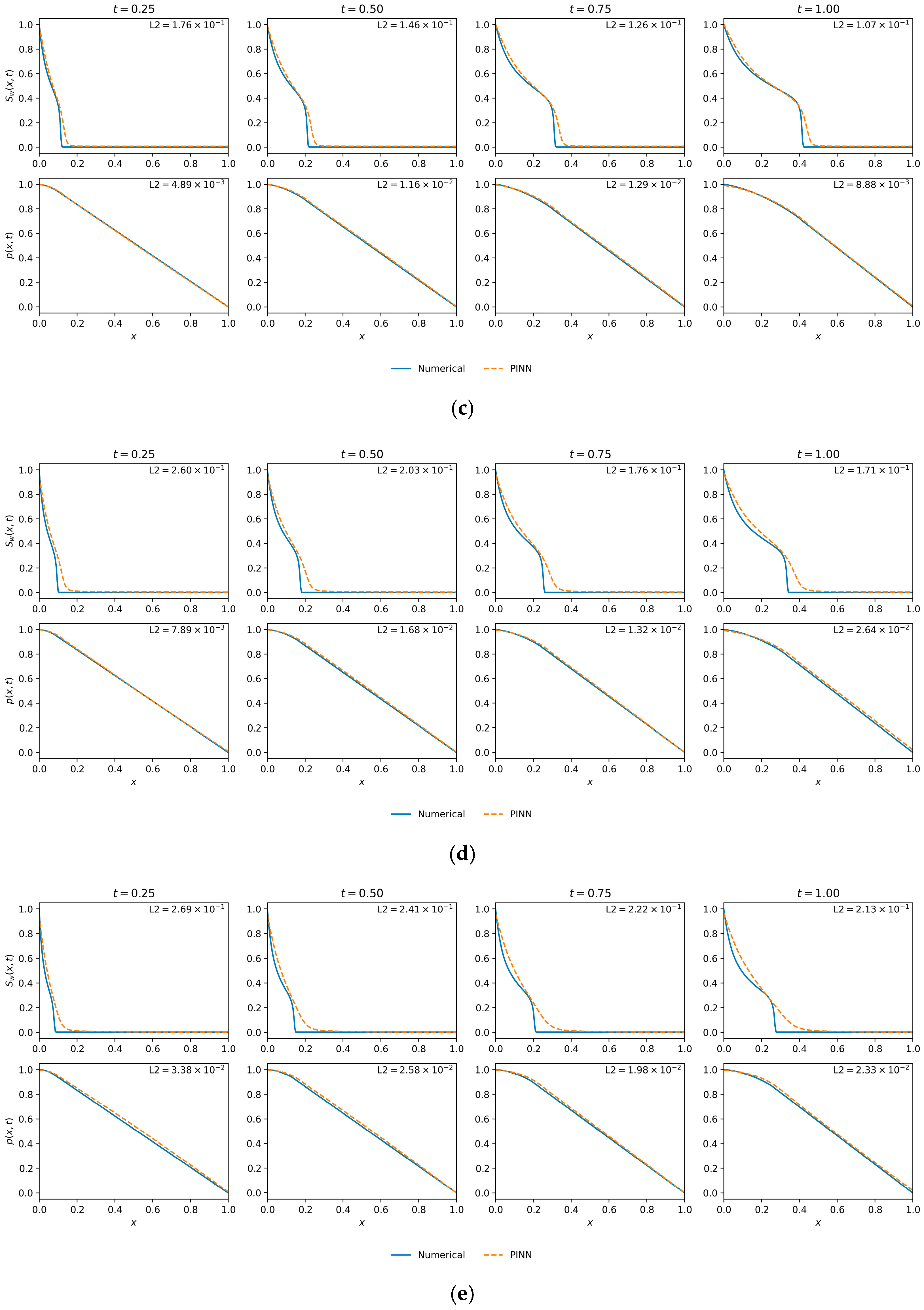
The qualitative predictions, presented in Figure 11, provide visual confirmation of these quantitative findings. Figure 11b () showcases the optimal case. The PINN solution is in near-perfect agreement with the numerical reference for both saturation and pressure, validating its high fidelity in this balanced regime.
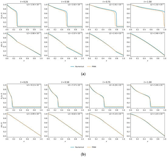
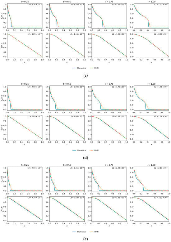
Figure 11.
Marginal saturation and pressure profile comparisons for M = 1, 3, 5, 7, and 10. (a) ; (b) ; (c) ; (d) ; (e) M = 10.
Figure 11c () illustrates the onset of performance degradation. While the pressure profile remains highly accurate, the saturation front exhibits a subtle but clear smearing and phase lag compared to the reference. This visual discrepancy is the physical manifestation of the increased L2 error and exemplifies the challenges posed by an increasingly convective flow.
An intriguing observation from the data is the divergence between the final training loss and the solution accuracy. While the case achieved the lowest final loss (), the case yielded a significantly lower saturation error. This highlights the complex nature of the loss landscape and reinforces that the L2 error against a ground-truth solution, rather than the loss value itself, is the definitive metric for evaluating physical fidelity. This analysis indicates that although the PINN framework produces stable solutions over a wide spectrum of mobility ratios, its predictive accuracy is highest when convective and diffusive forces are comparably balanced.
4.3. Sensitivity to Injection Pressure
The final investigation assesses the PINN’s sensitivity to the physical injection pressure (), a critical operational parameter that dictates the overall pressure gradient () and thus modifies the balance between convection and capillarity. The analysis was performed using the optimal baseline architecture ( = 200, = 50,000) for a fixed mobility ratio of . The complete results are summarized in Table 5.

Table 5.
Results for sensitivity analysis across different values of (.
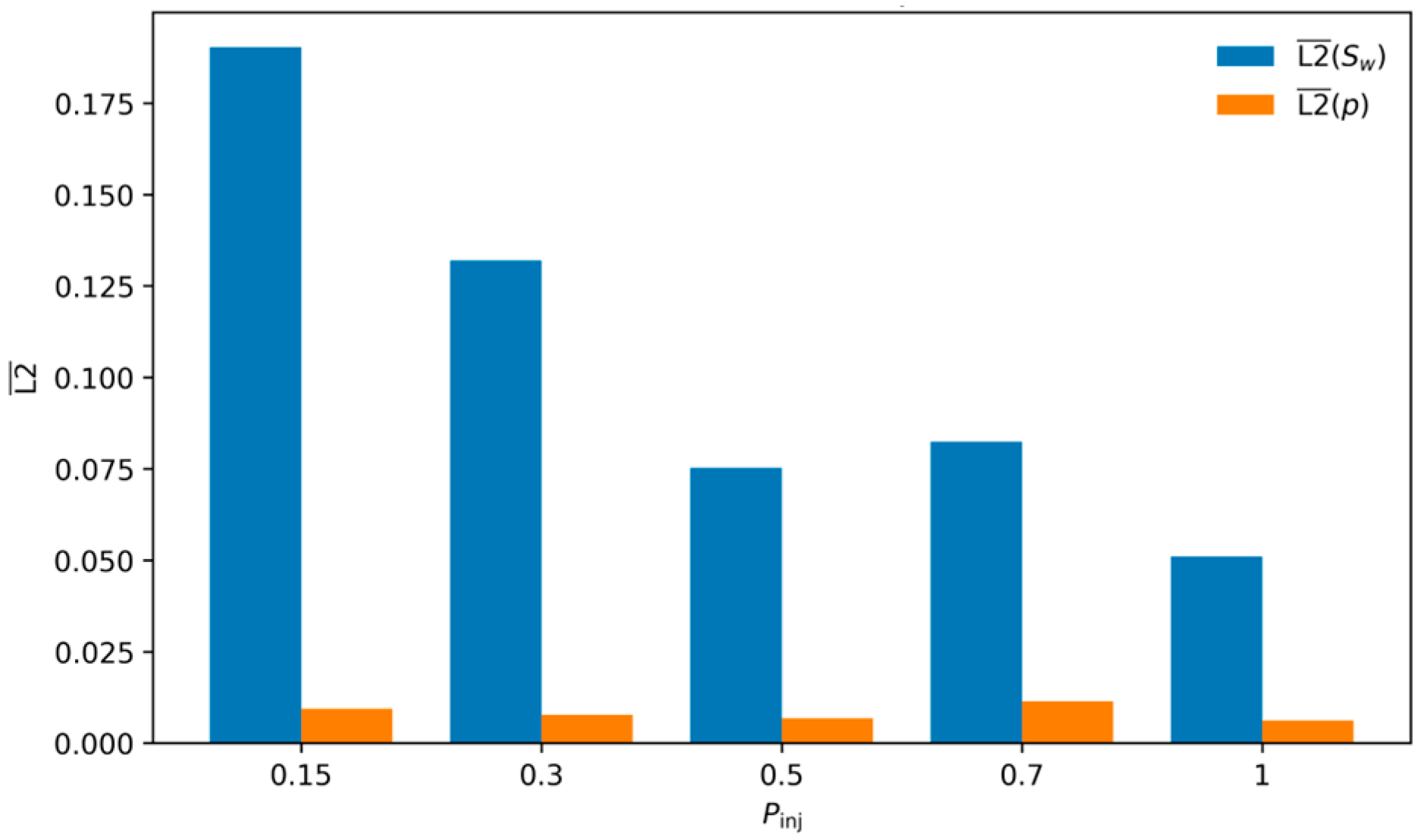
The results, visualized in the marginal effects plot in Figure 12, reveal a clear and significant trend: the PINN’s accuracy for the saturation field improves monotonically as the injection pressure increases. The highest error ( = ) occurs at the lowest injection pressure (), while the lowest error ( = ) is achieved at the highest pressure ( = 1.0).
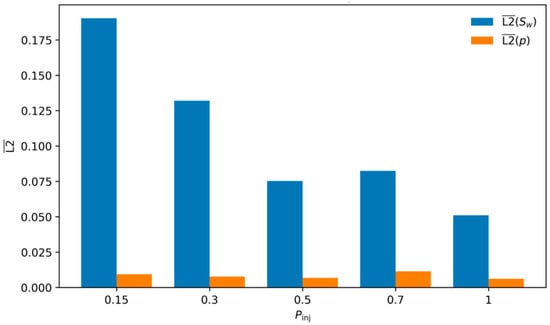
Figure 12.
Variation of the mean L2 errors in the wetting-phase saturation and pressure as a function of the injection pressure .
This behavior is explained by the underlying physics. A low injection pressure corresponds to a small pressure drop () and, consequently, a large dimensionless capillary prefactor (). This signifies a capillary-dominated regime, where the saturation front is broad and highly diffusive. As observed in the mobility ratio study, the PINN struggles to perfectly capture these highly dispersed fronts. Conversely, a high injection pressure leads to a large and a small , creating a convection-dominated regime. In this scenario, the front becomes steeper and more sharply defined. Unlike the “stiff” fronts caused by high mobility ratios, this convection-driven sharpening appears to be a feature that the PINN can resolve with very high accuracy, likely because the underlying pressure gradient provides a strong, well-defined signal for the network to learn.
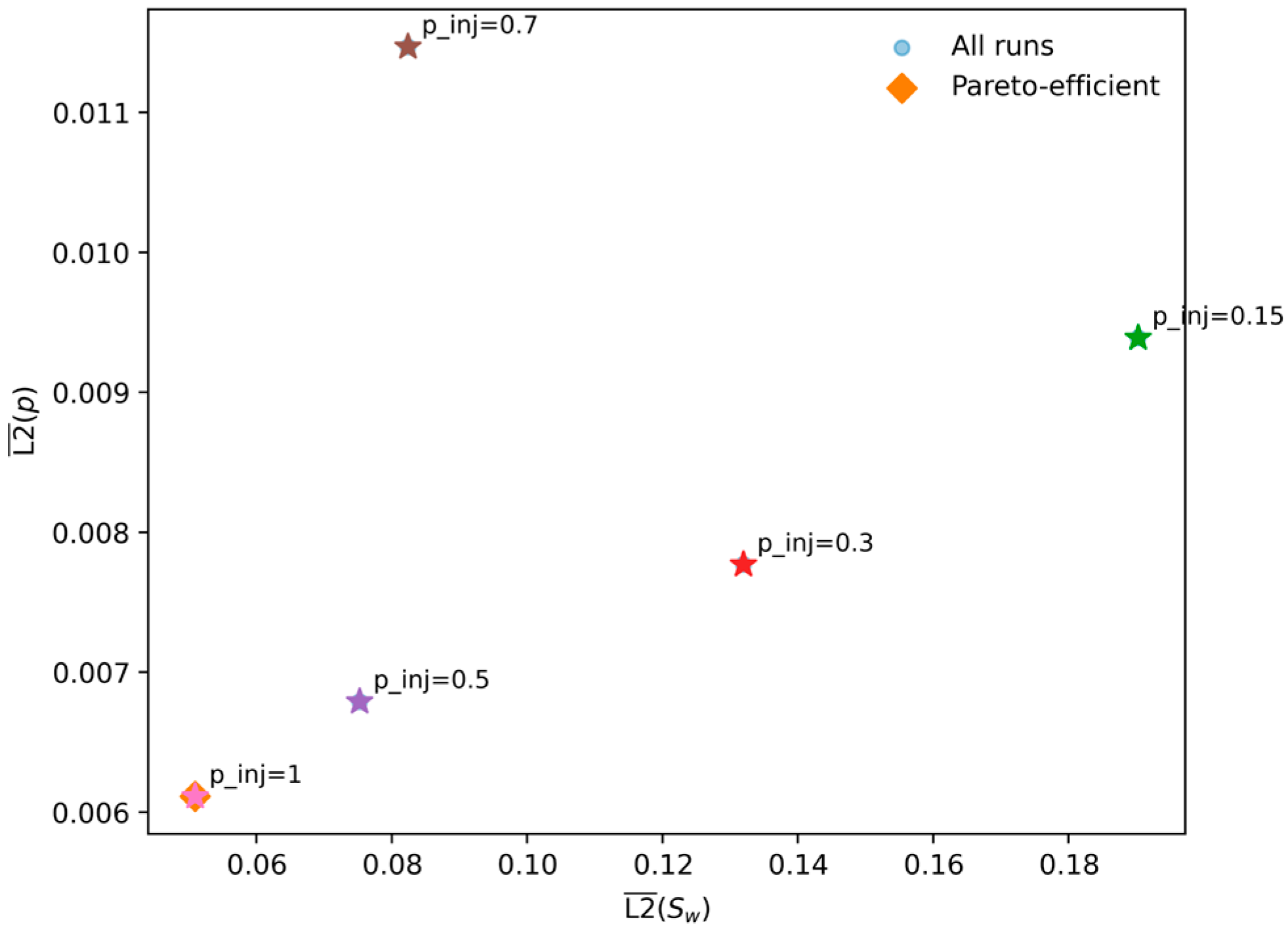
The Pareto plot in Figure 13 provides a compelling visualization of the performance trade-off. The Pareto front (i.e., the set of non-dominated trade-off solutions) defines the optimal compromise boundary among objectives [57]. The plot clearly shows that the = 1.0 case is Pareto-efficient, achieving the best performance in both saturation and pressure accuracy simultaneously. This makes it an unambiguously optimal configuration from a prediction standpoint.
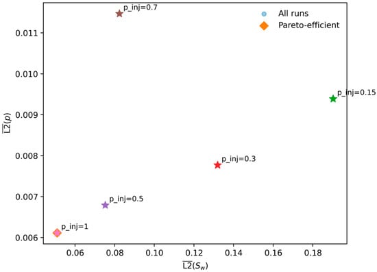
Figure 13.
Pareto plot of the mean L2 errors in pressure versus saturation for different injection pressures . Each point corresponds to one simulation, with Pareto-efficient configurations highlighted in orange.
The qualitative plots in Figure 14 provide visual confirmation of these quantitative results. Figure 14a ( = 0.3) represents the case with the lowest final training loss. While the pressure profile is well-matched, the saturation front shows a noticeable discrepancy, failing to fully capture the broad, diffusive nature of the front in this capillary-influenced regime. This visual mismatch explains the relatively high L2 error for saturation.
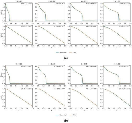
Figure 14.
Saturation and pressure profile comparisons from the injection pressure sensitivity study. (a) ( = 0.3): The model that achieved the lowest final training loss. (b) ( = 1.0): The model that achieved the highest physical fidelity, obtaining the lowest error for both saturation (Best by L2 ()) and pressure (Best by L2 (p)).
Figure 14b ( = 1.0) corresponds to the case with the lowest L2 error for both saturation and pressure. The visual agreement is exceptional. The PINN accurately resolves the steeper, convection-driven front at all time steps, demonstrating its validity and high fidelity in this physical regime.
This analysis denotes that the ML-PINN adapts successfully to different operational conditions and its accuracy is enhanced in convection-dominated flows driven by high pressure gradients. This suggests that the framework is particularly well-suited for modeling high-rate injection scenarios, where it can serve as a highly accurate predictive tool.
4.4. Computational Efficiency and Convergence
To assess the practical feasibility of the proposed PINN framework, we monitored the computational cost in terms of training time and iteration count. The total training time was primarily driven by the number of collocation points () and the physical stiffness of the problem setup.
Increasing the number of interior collocation points () imposes a direct but scalable computational cost. As shown in Table 3, increasing from 5000 to 50,000 (a increase) raised the training time from 117 s to 544 (a 4.6 increase). This sub-linear scaling indicates that the architecture leverages the GPU parallelism effectively. Given that this data increase reduced the saturation error by approximately 50%, the additional computational burden is justified.
The complexity of the underlying physics influenced the optimizer’s convergence rate. In the injection pressure sensitivity study (Table 5), the training times for the dense models ( = 50,000) ranged between 874 and 1174 s (approx. 15–20 min). Notably, the most physically “stiff” cases (e.g., lower injection pressure ) required more time (174 s) and iterations (21,000) compared to the convection-dominated case (906 s, 15,846 iterations), reflecting the difficulty of resolving broad capillary-diffusive tails.
Table 2 highlights the efficiency of the chosen shallow–wide architecture. The baseline model (10 layers, 50 neurons) converged in approximately 257 s with a low saturation error ). In contrast, deeper networks (30 layers) exhibited severe training instability. For example, the 30-layer, 30-neuron configuration terminated after only 1355 iterations with a high error (1.35), indicating a failure to converge. Even when 30-layer models did train for longer durations (e.g., the 30-layer, 20-neuron case took 318 s), they yielded errors an order of magnitude higher than the shallower baseline. This confirms that for the Muskat–Leverett system, representational capacity is better added via width (neurons) rather than depth.
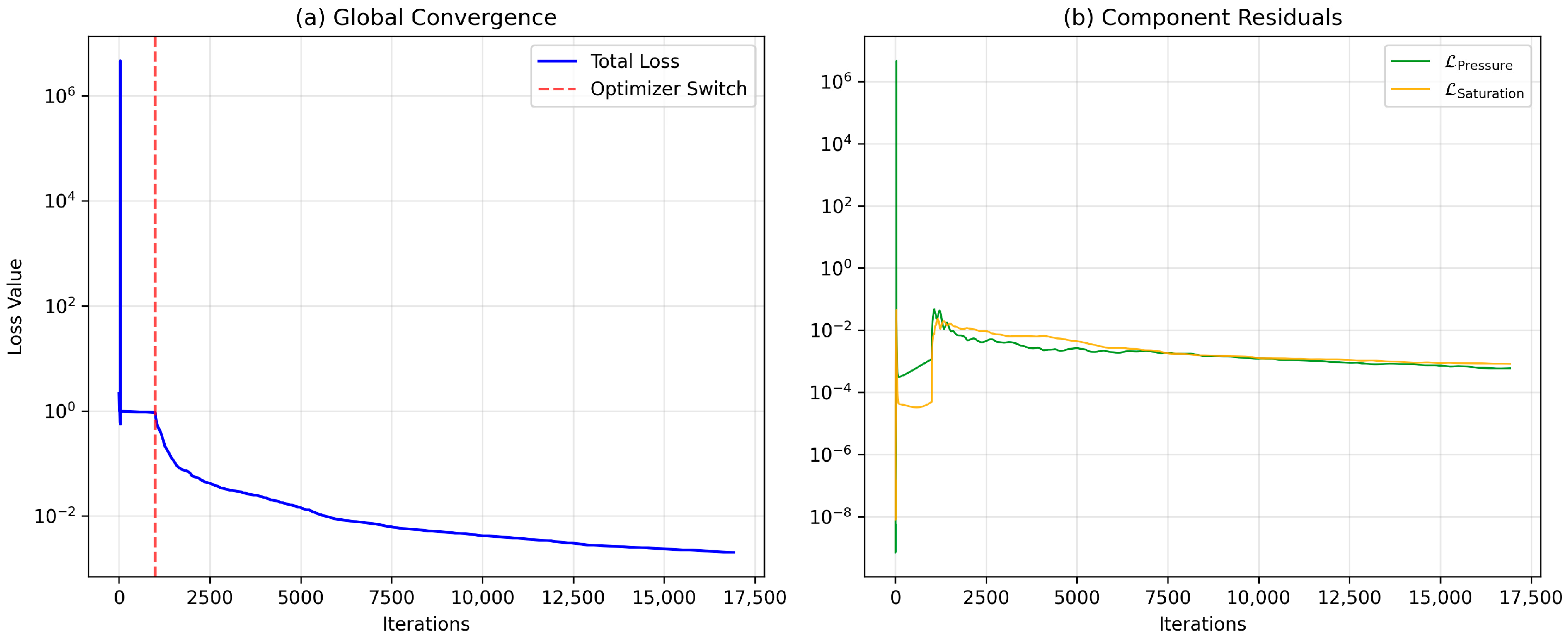
The training dynamics of the optimal baseline configuration are visualized in Figure 15. Figure 15a demonstrates the effectiveness of the two-stage optimization strategy. The initial Adam phase (iterations 0–1000) navigates the complex initial loss landscape, rapidly bringing the total loss to a stable basin ()). The transition to L-BFGS (marked by the red dashed line) triggers a sharp acceleration in convergence. By exploiting curvature information, the quasi-Newton optimizer resolves the ill-conditioned residuals that first-order methods struggle with, driving the final loss down by three orders of magnitude to .
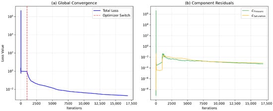
Figure 15.
Convergence history of the baseline PINN (M = 3, 10 layers, 50 neurons). (a) Global Convergence: The total loss (log scale) shows the distinct transition from the exploratory Adam phase to the high-precision L-BFGS phase (red dashed line). (b) Component Residuals: The decomposition of the PDE loss confirms that both pressure and saturation residuals are minimized simultaneously and remain well-balanced throughout the optimization.
Finally, regarding hardware requirements, the peak GPU memory footprint for the dense baseline model () was recorded at 4.78 GB. This consumption remains well within the capacity of standard consumer-grade GPUs (typically 8 GB or higher), confirming that the method is not hardware-bound. While the dense collocation grid increases memory load compared to standard 1D benchmarks, the cost is justifiable given the 50% error reduction, and the method retains significant headroom for scaling to larger batch sizes or higher-dimensional domains.
5. Discussion
Taken together, the results delineate a coherent recipe for learning the coupled Muskat–Leverett dynamics with a single shared network for and (considering capillarity): enforce the physics densely, favor shallow–wide architectures, and regularize just enough to negotiate stiffness without erasing the front. The baseline numerical references (IMPES) make the target unambiguous, and the relative L2 metrics keep the assessment tied to physical fidelity rather than internal optimization surrogates. Within this frame, the evidence points to a model that is demonstrably accurate on pressure and whose ultimate difficulty lies in reconstructing the saturation front across regimes.
The architecture scan provides quantitative evidence that network depth acts as the primary bottleneck for optimization stability in this coupled system. As detailed in Table 2, increasing depth from 10 to 30 layers did not merely reduce accuracy; it caused fundamental optimization failures. Specifically, the 30-layer configuration (30 layers 30 neurons) terminated prematurely after only 1355 iterations with a final loss of , compared to the 14,646 iterations and loss achieved by the 10-layer baseline. This premature stagnation at a high error plateau is a hallmark of gradient pathology (vanishing or exploding gradients) characteristic of deep, un-residual networks applied to stiff PDEs. In contrast, the shallow–wide architectures maintained healthy convergence rates throughout the L-BFGS phase, allowing the optimizer to resolve the high-frequency components of the saturation front. Thus, the superiority of the 10-layer model is not just a matter of final accuracy, but of learnability: the shallower graph preserves the gradient signal required to navigate the stiff loss landscape of the Muskat–Leverett system.
The role of artificial diffusion follows the same logic, effectively serving as a control on the trade-off between numerical stability and physical fidelity. Larger values (e.g., stabilize convergence across hyperparameters but result in consistently higher saturation errors; in this regime, the artificial numerical diffusion begins to overshadow the physical capillary forces, leading to an artificially smeared, non-physical front. Conversely, smaller values (e.g., ) theoretically allow for a sharper recovery of the front but invite severe optimization failures, as the network struggles to resolve high-frequency spectral components without sufficient regularization. The observation that attains the best saturation accuracy suggests it represents the empirical vanishing viscosity limit—sufficient to dampen gradient noise without dominating the global transport dynamics defined by the physical pressure–saturation coupling. The scientifically relevant criterion, therefore, is not the final loss value but the out-of-sample reconstruction of the front, hence selecting by rather than by the composite training objective.
The factorial study on sampling density isolates the true lever: the number of interior collocation points overwhelmingly controls accuracy, whereas the number of boundary/initial data points exerts a weaker, noisy effect once minimal constraints are satisfied. As increases from 5000 to 50,000, the saturation error drops by roughly a factor of two, while the pressure error remains uniformly low across the board. This is exactly what a physicist would predict. In a problem where the interior PDE is the dominant source of information, and where the target structures are fronts rather than smooth harmonic fields, blanketing the space-time domain with residual enforcement is the only way to reduce aliasing of the conservation law.
Two parameter studies clarify how the physics shapes learnability. Varying the mobility ratio M produces a non-monotone accuracy curve, with a clear optimum at M = 3. This highlights a balance between physical distinguishability and the network’s spectral bias. At M = 1, capillarity dominates, creating a broad front with long spatial tails; capturing these subtle, low-magnitude saturation changes over a large domain proves difficult for the residual loss to localize. Conversely, at large M (e.g., M = 10), the flow is strongly unstable and convection-dominated, leading to steep, shock-like gradients. Deep networks suffer from spectral bias, a tendency to learn low-frequency components faster than high-frequency discontinuities, making these sharp fronts difficult to approximate without Gibbs-like oscillations or phase lags. The balanced case at M = 3 represents the optimal sweet spot: the front is sufficiently sharp to be distinct (unlike M = 1) yet possesses enough capillary width to be resolved by smooth activation functions without triggering spectral bias (unlike M = 10).
By contrast, sweeping the injection pressure yields a monotone improvement in saturation accuracy as increases. Superficially, this may appear inconsistent with the high- degradation; both sharpen the front. Superficially, this may appear inconsistent with the degradation seen at high M, as both scenarios sharpen the front. However, the physical mechanism differs. Increasing creates a larger global pressure drop, resulting in higher Darcy velocities and a stronger advective drive throughout the domain. While this theoretically steepens the saturation front, the strong, non-zero pressure gradients provide a robust supervisory signal during backpropagation. The network receives unambiguous directional information for the flux, effectively improving the signal-to-noise ratio of the loss gradients and preventing the optimization stagnation often observed in low-gradient, diffusion-dominated regimes. Thus, increasing produces a front that is sharper yet better conditioned from the optimizer’s perspective.
A recurrent theme across all experiments is the asymmetry between fields: pressure is uniformly “easy,” saturation “hard.” The pressure equation is elliptic-like and produces smooth solutions; the saturation equation remains an advection–diffusion conservation law even with capillarity. It is therefore appropriate to select baselines by and treat as a necessary but insufficient condition. The occasional mismatch between the smallest final training loss and the smallest simply underscores the misalignment between a composite residual objective and the task-relevant error. In practice, this counsels toward calibration of residual weights or gradient balancing and toward model selection on a validation rather than on the raw optimizer endpoint.
In this work, we did not optimize either the IMPES reference implementation or the PINN code for wall-clock performance, and we therefore do not report a speedup ratio. In its present form, a separate PINN is trained for each physical regime , analogous to running a separate IMPES simulation per case. The main benefit of the Muskat–Leverett PINN is thus not reduced offline cost for a single forward solve, but a mesh-free, differentiable surrogate of the coupled pressure–saturation fields that can be evaluated very cheaply at arbitrary space–time points and reused for visualization, sensitivity analysis, or potential inverse problems once training is complete.
Our results also contextualize the proposed framework within the broader landscape of PINN variants. While recent literature has emphasized architectural complexity, such as domain decomposition (cPINNs/XPINNs) to handle local stiffness [29,30], or adaptive loss weighting (e.g., GradNorm, NTK) to resolve competing objectives, our findings suggest that for the coupled Muskat–Leverett system, a parsimonious approach is sufficient.
First, regarding loss balancing: The convergence history in Figure 15b demonstrates that the pressure and saturation residuals naturally decay in unison without adaptive weighting. This indicates that the explicitly coupled formulation, where pressure gradients drive saturation transport, inherently preconditions the optimization landscape, rendering computationally expensive gradient-balancing schemes unnecessary in this regime.
Second, regarding adaptive sampling: While adaptive strategies are often required to resolve shocks in the inviscid Buckley–Leverett limit, Table 3 confirms that dense uniform (LHS) sampling () is sufficient to capture the capillary-regularized front with high fidelity (). Given that dense sampling on a GPU is computationally cheap compared to the overhead of iterative resampling loops or sub-domain stitching required by cPINNs, our ‘brute-force’ density approach offers a more implementable and efficient baseline for engineering applications.
Finally, the methodology choices that enabled these outcomes are not incidental. Training a single shared-parameter network for with the added complexity of capillarity appears to encourage a physically consistent coupling: the network cannot improve one field without implicitly honoring its influence on the other through mobilities and capillarity. The bounded saturation head eliminates excursions outside and removes a class of unphysical minima that often derail PINN training in stiff regimes. And dense interior enforcement, especially at , constitutes the decisive ingredient that turns the PINN from a qualitative emulator into a quantitative solver for this system.
To clearly portray the learning dynamics of the PINN framework, the scope of this study was intentionally focused on a foundational case: the 1D, homogeneous, incompressible Muskat–Leverett system with a static capillary pressure law. This controlled setting provides unambiguous insights but naturally defines the boundaries for external validity and highlights clear avenues for future research. The present methodology shows strong performance under the tested conditions, but further work could improve its numerical stability and efficiency. For instance, while dense collocation proved highly effective, its computational expense could be mitigated by implementing residual- or front-adaptive sampling strategies. Similarly, the composite loss function, while successful, could be better aligned with the primary physical challenge of resolving the saturation front through the adoption of gradient-balancing or uncertainty-weighting schemes.
Looking forward, the logical extension of this work is to broaden its physical and geometric complexity. This includes progressing to 2D/3D domains with heterogeneous and anisotropic permeability, incorporating gravity and hysteresis, and modeling more advanced physics such as dynamic capillarity. A crucial step in this progression will be to enforce mass conservation more explicitly, either through conservative PINN formulations (e.g., cPINNs) or by incorporating hard flux-continuity constraints. Furthermore, transitioning from a research tool to a practical surrogate model will involve investigating operator-learning architectures (e.g., DeepONet, FNO) that can generalize across physical parameters after being trained on a suite of high-fidelity PINN solutions. Together, these advancements will build upon the foundational insights of this study to extend the method’s applicability toward field-realistic scenarios.
6. Conclusions
We presented a Physics-Informed Neural Network (PINN) framework that jointly predicts wetting pressure and wetting saturation for the coupled Muskat–Leverett system and systematically exploits the classical capillary-pressure term in the pressure equation as the primary, physically motivated regularizer of the saturation front. In contrast to AV-based PINN formulations, we avoid heavy reliance on non-physical artificial viscosity by keeping the governing PDEs in their capillarity-regularized form and adding only a small numerical diffusion term in the saturation residual as a training stabilizer when needed. We further introduced a selective saturation-clamping head to guarantee admissible in stiff regimes.
A systematic study clarified which design choices matter most. Shallow–wide networks (10 layers 50 neurons) consistently outperformed deeper architectures, and interior physics enforcement dominated data requirements: increasing collocation points from to halved the saturation error, while boundary data had a comparatively minor effect once basic constraints were satisfied. Parametric sweeps showed that accuracy is highest at an intermediate mobility ratio (), where convection and capillarity are comparably balanced, and that raising injection pressure (larger ) improves accuracy monotonically, yielding sharper but well-conditioned fronts that the network can learn reliably. Across all experiments, pressure was consistently easy to learn, while saturation set the standard for model selection; accordingly, we prioritize as the primary fidelity metric.
These results provide a practical recipe for PINN solvers of coupled two-phase flow with capillarity: (i) use physical capillarity as the main regularization mechanism; (ii) favor shallow–wide architectures over deep ones; (iii) allocate budget to dense interior enforcement; (iv) apply bounded outputs only when stiffness requires it; and (v) evaluate and select models by the harder error to optimize (in our case, saturation error), not optimizer loss. Under these choices, the framework serves as a credible surrogate that produces accurate pressure–saturation fields and enables sensitivity analysis across mobility ratio and injection pressure.
This work was intentionally scoped to a 1D, homogeneous, incompressible setting with a static law; as such, its conclusions are most directly applicable to that regime. Natural extensions include (a) 2D/3D domains with heterogeneous and anisotropic permeability, gravity, and hysteresis; (b) dynamic capillarity models; (c) explicit conservation via conservative PINN variants or hard flux-continuity constraints; (d) residual- or front-adaptive sampling to reduce training cost; (e) loss-term balancing or uncertainty-weighting aligned to fidelity; and (f) operator learning trained on PINN-generated datasets for fast, parameter-generalizing surrogates. Pursuing these directions should extend the method’s accuracy and efficiency toward field-scale applications while retaining the physics-consistent behavior demonstrated here.
Author Contributions
Conceptualization, T.I. and A.K.; methodology, T.I., A.K., S.D.B. and Y.K.; software, S.D.B. and B.A.; validation, T.I., Y.K. and Z.Z.; formal analysis, T.I. and A.K.; investigation, T.I., A.K., B.A. and Z.Z.; resources, B.A., A.K. and Z.Z.; data curation, A.K., B.A. and S.D.B.; writing—original draft preparation, T.I., S.D.B. and Y.K.; writing—review and editing, T.I., A.K., S.D.B., Z.Z., B.A. and Y.K.; visualization, T.I., S.D.B. and Y.K., and supervision, T.I., Y.K., B.A. and Z.Z.; project administration, T.I., A.K. and B.A.; funding acquisition, A.K. and Z.Z. All authors have read and agreed to the published version of the manuscript.
Funding
This work was funded by the Committee of Science of the Ministry of Science and Higher Education of the Republic of Kazakhstan (Grant number AP19676964).
Institutional Review Board Statement
Not applicable.
Informed Consent Statement
Not applicable.
Data Availability Statement
The PINN training does not rely on any external dataset; collocation, initial, and boundary points are generated procedurally from the governing equations. The numerical reference solutions used for evaluation (IMPES fields and associated input files) are available from the authors upon reasonable request to the corresponding author. No proprietary or confidential data were used.
Conflicts of Interest
The authors declare no conflicts of interest.
References
- Agbalaka, C.; Dandekar, A.Y.; Patil, S.L.; Khataniar, S.; Hemsath, J.R. The Effect of Wettability on Oil Recovery: A Review. In Proceedings of the SPE Asia Pacific Oil and Gas Conference and Exhibition, Perth, Australia, 20–22 October 2008; OnePetro: Richardson, TX, USA, 2008. [Google Scholar] [CrossRef]
- Wenck, N.; Muggeridge, A.; Jackson, S.; An, S.; Krevor, S. The impact of capillary heterogeneity on CO2 plume migration at the Endurance CO2 storage site in the UK. Geoenergy 2025, 3, geoenergy2024-029. [Google Scholar] [CrossRef]
- Muskat, M. The Flow of Homogeneous Fluids Through Porous Media, 1st ed.; Springer: New York, NY, USA, 1937. [Google Scholar]
- Buckley, S.E.; Leverett, M.C. Mechanism of Fluid Displacement in Sands. Trans. AIME 1942, 146, 107–116. [Google Scholar] [CrossRef]
- Welge, H.J. A Simplified Method for Computing Oil Recovery by Gas or Water Drive. J. Pet. Technol. 1952, 4, 91–98. [Google Scholar] [CrossRef]
- Leverett, M.C. Capillary Behavior in Porous Solids. Trans. AIME 1941, 142, 152–169. [Google Scholar] [CrossRef]
- Saffman, P.G.; Taylor, G.I. The penetration of a fluid into a porous medium or Hele-Shaw cell containing a more viscous liquid. Proc. R. Soc. Lond. A 1958, 245, 312–329. [Google Scholar] [CrossRef]
- Homsy, G.M. Viscous Fingering in Porous Media. Annu. Rev. Fluid Mech. 1987, 19, 271–311. [Google Scholar] [CrossRef]
- Bear, J. Dynamics of Fluids in Porous Media. Soil Sci. 1975, 120, 162. [Google Scholar] [CrossRef]
- Helmig, R. Multiphase Flow and Transport Processes in the Subsurface: A Contribution to the Modeling of Hydrosystems; Environmental Engineering; Springer: Berlin/Heidelberg, Germany, 1997; ISBN 978-3-540-62703-6. [Google Scholar]
- Blunt, M.J. Multiphase Flow in Permeable Media: A Pore-Scale Perspective, 1st ed.; Cambridge University Press: Cambridge, UK, 2016; ISBN 978-1-107-09346-1. [Google Scholar] [CrossRef]
- Majid Hassanizadeh, S.; Gray, W.G. Toward an improved description of the physics of two-phase flow. Adv. Water Resour. 1993, 16, 53–67. [Google Scholar] [CrossRef]
- Joekar-Niasar, V.; Hassanizadeh, S.M.; Dahle, H.K. Non-equilibrium effects in capillarity and interfacial area in two-phase flow: Dynamic pore-network modelling. J. Fluid Mech. 2010, 655, 38–71. [Google Scholar] [CrossRef]
- Spayd, K.; Shearer, M. The Buckley–Leverett Equation with Dynamic Capillary Pressure. SIAM J. Appl. Math. 2011, 71, 1088–1108. [Google Scholar] [CrossRef]
- Liang, R.; Fan, X.; Luo, X.; Sun, S.; Zhu, X. Improved IMPES Scheme for the Simulation of Incompressible Three-Phase Flows in Subsurface Porous Media. Energies 2021, 14, 2757. [Google Scholar] [CrossRef]
- Makhmut, E. Parallel Implementation of Muskat-Levertt Equation Using CUDA. J. Math. Mech. Comput. Sci. 2023, 119, 104–116. [Google Scholar] [CrossRef]
- Chavent, G.; Jaffré, J. Mathematical Models and Finite Elements for Reservoir Simulation: Single Phase, Multiphase and Multicomponent Flows Through Porous Media; Studies in Mathematics and Its Applications; North-Holland: Amsterdam, The Netherlands, 1986; ISBN 978-0-08-087538-5. [Google Scholar]
- Monteagudo, J.E.P.; Firoozabadi, A. Comparison of fully implicit and IMPES formulations for simulation of water injection in fractured and unfractured media. Int. J. Numer. Methods Eng. 2007, 69, 698–728. [Google Scholar] [CrossRef]
- Wang, Y.; Chung, E.; Sun, S. Physics-Preserving IMPES Based Multiscale Methods for Immiscible Two-Phase Flow in Highly Heterogeneous Porous Media. J. Sci. Comput. 2025, 102, 38. [Google Scholar] [CrossRef]
- Chen, H.; Kou, J.; Sun, S.; Zhang, T. Fully mass-conservative IMPES schemes for incompressible two-phase flow in porous media. Comput. Methods Appl. Mech. Eng. 2019, 350, 641–663. [Google Scholar] [CrossRef]
- Raissi, M.; Perdikaris, P.; Karniadakis, G.E. Physics-informed neural networks: A deep learning framework for solving forward and inverse problems involving nonlinear partial differential equations. J. Comput. Phys. 2019, 378, 686–707. [Google Scholar] [CrossRef]
- Fuks, O.; Tchelepi, H.A. Limitations of Physics Informed Machine Learning for Nonlinear Two-Phase Transport in Porous Media. J. Mach. Learn Model Comput. 2020, 1, 19–37. [Google Scholar] [CrossRef]
- Wang, T.; Zhao, B.; Gao, S.; Yu, R. Understanding the difficulty of solving Cauchy problems with PINNs. In Proceedings of the 6th Annual Learning for Dynamics & Control Conference, Oxford, UK, 15–17 July 2024; PMLR: Cambridge, MA, USA, 2024; pp. 453–465. [Google Scholar]
- Xu, Z.-Q.J.; Zhang, L.; Cai, W. On understanding and overcoming spectral biases of deep neural network learning methods for solving PDEs. J. Comput. Phys. 2025, 530, 113905. [Google Scholar] [CrossRef]
- Abbasi, J.; Jagtap, A.D.; Moseley, B.; Hiorth, A.; Andersen, P.Ø. Challenges and advancements in modeling shock fronts with physics-informed neural networks: A review and benchmarking study. Neurocomputing 2025, 657, 131440. [Google Scholar] [CrossRef]
- Zhao, Z.; Ding, X.; Prakash, B.A. PINNsFormer: A Transformer-Based Framework for Physics-Informed Neural Networks. arXiv 2023, arXiv:2307.11833. [Google Scholar]
- Coutinho, E.J.R.; Dall’Aqua, M.; McClenny, L.; Zhong, M.; Braga-Neto, U.; Gildin, E. Physics-informed neural networks with adaptive localized artificial viscosity. J. Comput. Phys. 2023, 489, 112265. [Google Scholar] [CrossRef]
- Zhang, J.; Braga-Neto, U.; Gildin, E. Physics-Informed Neural Networks for Multiphase Flow in Porous Media Considering Dual Shocks and Interphase Solubility. Energy Fuels 2024, 38, 17781–17795. [Google Scholar] [CrossRef]
- Jagtap, A.D.; Kharazmi, E.; Karniadakis, G.E. Conservative physics-informed neural networks on discrete domains for conservation laws: Applications to forward and inverse problems. Comput. Methods Appl. Mech. Eng. 2020, 365, 113028. [Google Scholar] [CrossRef]
- Jagtap, A.D.; Karniadakis, G.E. Extended Physics-Informed Neural Networks (XPINNs): A Generalized Space-Time Domain Decomposition Based Deep Learning Framework for Nonlinear Partial Differential Equations. Commun. Comput. Phys. 2020, 28, 2002–2041. [Google Scholar] [CrossRef]
- Rodriguez-Torrado, R.; Ruiz, P.; Cueto-Felgueroso, L.; Green, M.C.; Friesen, T.; Matringe, S.; Togelius, J. Physics-informed attention-based neural network for hyperbolic partial differential equations: Application to the Buckley–Leverett problem. Sci. Rep. 2022, 12, 7557. [Google Scholar] [CrossRef] [PubMed]
- Shan, L.; Liu, C.; Liu, Y.; Tu, Y.; Dong, L.; Hei, X. Physics-informed machine learning for solving partial differential equations in porous media. Adv. Geo-Energy Res. 2023, 8, 37–44. [Google Scholar] [CrossRef]
- Zhao, J.; Wu, J.; Wang, H.; Xia, Y.; Cai, J. Single phase flow simulation in porous media by physical-informed Unet network based on lattice Boltzmann method. J. Hydrol. 2024, 639, 131501. [Google Scholar] [CrossRef]
- Daribayev, B.; Mukhanbet, A.; Makhmut, E.; Azatbekuly, N.; Imankulov, T. Quantum–Classical Hybrid Architecture for Solving the Muskat–Leverett Model. IET Quantum Commun. 2025, 6, e70022. [Google Scholar] [CrossRef]
- Lu, L.; Pestourie, R.; Yao, W.; Wang, Z.; Verdugo, F.; Johnson, S.G. Physics-Informed Neural Networks with Hard Constraints for Inverse Design. SIAM J. Sci. Comput. 2021, 43, B1105–B1132. [Google Scholar] [CrossRef]
- Chen, S.; Liu, Z.; Zhang, W.; Yang, J. A Hard-Constraint Wide-Body Physics-Informed Neural Network Model for Solving Multiple Cases in Forward Problems for Partial Differential Equations. Appl. Sci. 2024, 14, 189. [Google Scholar] [CrossRef]
- Zhang, Z. A physics-informed deep convolutional neural network for simulating and predicting transient Darcy flows in heterogeneous reservoirs without labeled data. J. Pet. Sci. Eng. 2022, 211, 110179. [Google Scholar] [CrossRef]
- Li, J.; Zhang, D.; Wang, N.; Chang, H. Deep Learning of Two-Phase Flow in Porous Media via Theory-Guided Neural Networks. SPE J. 2022, 27, 1176–1194. [Google Scholar] [CrossRef]
- Kenzhebek, Y.; Imankulov, T.; Bekele, S.D.; Panfilova, I.; Akhmed-Zaki, D. Coupled pressure and saturation prediction for two-phase flow in porous media using physics-informed neural networks (PINNs). Comput. Methods Appl. Mech. Eng. 2025, 446, 118229. [Google Scholar] [CrossRef]
- Chakraborty, A.; Rabinovich, A.; Moreno, Z. Physics-informed neural networks for modeling two-phase steady state flow with capillary heterogeneity at varying flow conditions. Adv. Water Resour. 2024, 185, 104639. [Google Scholar] [CrossRef]
- Chen, H.; Sun, S. A new physics-preserving IMPES scheme for incompressible and immiscible two-phase flow in heterogeneous porous media. J. Comput. Appl. Math. 2021, 381, 113035. [Google Scholar] [CrossRef]
- Anagnostopoulos, S.J.; Toscano, J.D.; Stergiopulos, N.; Karniadakis, G.E. Learning in PINNs: Phase transition, diffusion equilibrium, and generalization. Neural Netw. 2026, 193, 107983. [Google Scholar] [CrossRef]
- Hanna, J.M.; Aguado, J.V.; Comas-Cardona, S.; Askri, R.; Borzacchiello, D. Sensitivity analysis using Physics-informed neural networks. Eng. Appl. Artif. Intell. 2024, 135, 108764. [Google Scholar] [CrossRef]
- Chen, Z.; Huan, G.; Ma, Y. Computational Methods for Multiphase Flows in Porous Media; Society for Industrial and Applied Mathematics: Philadelphia, PA, USA, 2006; ISBN 978-0-89871-606-1. [Google Scholar] [CrossRef]
- Aziz, K.; Settari, A. Petroleum Reservoir Simulation; Society of Petroleum Engineers; Springer: Dordrecht, The Netherlands, 1979; ISBN 978-1-61399-964-6. [Google Scholar] [CrossRef]
- Peaceman, D.W. Fundamentals of Numerical Reservoir Simulation; Developments in Petroleum Science; Elsevier: Amsterdam, The Netherlands, 1977; Volume 6, ISBN 978-0-444-41578-3. [Google Scholar]
- Shields, M.D.; Zhang, J. The generalization of Latin hypercube sampling. Reliab. Eng. Syst. Saf. 2016, 148, 96–108. [Google Scholar] [CrossRef]
- Dwivedi, V.; Parashar, N.; Srinivasan, B. Distributed physics informed neural network for data-efficient solution to partial differential equations. Neurocomputing 2021, 420, 299–316. [Google Scholar] [CrossRef]
- Wu, C.; Zhu, M.; Tan, Q.; Kartha, Y.; Lu, L. A comprehensive study of non-adaptive and residual-based adaptive sampling for physics-informed neural networks. Comput. Methods Appl. Mech. Eng. 2023, 403, 115671. [Google Scholar] [CrossRef]
- McKay, M.D.; Beckman, R.J.; Conover, W.J. Comparison of Three Methods for Selecting Values of Input Variables in the Analysis of Output from a Computer Code. Technometrics 1979, 21, 239–245. [Google Scholar] [CrossRef]
- Kingma, D.P.; Ba, J. Adam: A Method for Stochastic Optimization. arXiv 2014, arXiv:1412.6980. [Google Scholar]
- Byrd, R.H.; Lu, P.; Nocedal, J.; Zhu, C. A Limited Memory Algorithm for Bound Constrained Optimization. SIAM J. Sci. Comput. 1995, 16, 1190–1208. [Google Scholar] [CrossRef]
- Rathore, P.; Lei, W.; Frangella, Z.; Lu, L.; Udell, M. Challenges in training PINNs: A loss landscape perspective. In Proceedings of the 41st International Conference on Machine Learning, Vienna, Austria, 21–27 July 2024; JMLR.org: San Diego, CA, USA, 2024; Volume 235, pp. 42159–42191. [Google Scholar]
- Markidis, S. The Old and the New: Can Physics-Informed Deep-Learning Replace Traditional Linear Solvers? Front. Big Data 2021, 4, 669097. [Google Scholar] [CrossRef] [PubMed]
- Cuomo, S.; Di Cola, V.S.; Giampaolo, F.; Rozza, G.; Raissi, M.; Piccialli, F. Scientific Machine Learning Through Physics–Informed Neural Networks: Where we are and What’s Next. J. Sci. Comput. 2022, 92, 88. [Google Scholar] [CrossRef]
- Evans, L.C. Partial Differential Equations, 2nd ed.; Graduate Studies in Mathematics; American Mathematical Society: Providence, RI, USA, 2022; ISBN 978-1-4704-6942-9. [Google Scholar]
- Emmerich, M.T.M.; Deutz, A.H. A tutorial on multiobjective optimization: Fundamentals and evolutionary methods. Nat. Comput. 2018, 17, 585–609. [Google Scholar] [CrossRef]
Disclaimer/Publisher’s Note: The statements, opinions and data contained in all publications are solely those of the individual author(s) and contributor(s) and not of MDPI and/or the editor(s). MDPI and/or the editor(s) disclaim responsibility for any injury to people or property resulting from any ideas, methods, instructions or products referred to in the content. |
© 2025 by the authors. Licensee MDPI, Basel, Switzerland. This article is an open access article distributed under the terms and conditions of the Creative Commons Attribution (CC BY) license (https://creativecommons.org/licenses/by/4.0/).

