Deep Model Based on Mamba Fusion Multi-Scale Convolution LSTM for OSA Severity Grading

Abstract

Obstructive sleep apnea (OSA) affects nearly one billion individuals worldwide, and its rising prevalence exacerbates cardiovascular and metabolic burdens. Although overnight polysomnography (PSG) is the diagnosis gold standard, its cost and procedural complexity constrain population-level deployment. To address this gap, an end-to-end model is developed. It operates directly on full-night peripheral oxygen saturation (SpO₂) sequences sampled at 1 Hz. The model integrates multi-scale convolution, state space modeling, and channel-wise attention to classify obstructive sleep apnea severity into four levels. Evaluated on the Sleep Heart Health Study cohorts, the approach achieved overall accuracies of 80.51% on SHHS1 and 76.61% on SHHS2, with mean specificity exceeding 92%. These results suggest that a single-channel SpO₂ signal is sufficient for four-class OSA classification without extensive preprocessing or additional PSG channels. This approach may enable low-cost, large-scale home screening and provide a basis for future multimodal, real-time monitoring.

1. Introduction

Sleep apnea (SA) is a common sleep-related respiratory disorder characterized by recurrent episodes of apnea or hypopnea during sleep and is associated with cardiovascular disease, diabetes, and dementia (Punjabi [1]). SA is typically classified into three types: obstructive, central, and mixed, with obstructive sleep apnea (OSA) being the most prevalent. OSA severity is commonly assessed by the apnea–hypopnea index (AHI) and categorized into four levels: normal, mild, moderate, and severe. Epidemiologic studies estimate that ~24% of men and 9% of women are affected by OSA, yet many cases remain undiagnosed (Dempsey [2]). Overnight polysomnography (PSG) is widely regarded as the diagnosis gold standard, monitoring multiple physiologic signals including respiratory airflow, arterial oxygen saturation (SpO₂), and body position. However, PSG is time-consuming, operationally complex, and equipment-intensive, which hinders broad adoption and may contribute to diagnosis delays (Shojaee [3]). Given the rising global burden of chronic disease, early identification of OSA remains challenging, and there is an urgent need for simple, cost-effective, automated screening and diagnosis methods. To address these limitations, a multi-scale convolution (MSC)–long-short term memory (LSTM) parallel architecture with Mamba embeddings is proposed for automatic OSA severity classification. Figure 1 provides an overview of the proposed work, with its main contributions as follows: (1) end-to-end inference on unsegmented overnight SpO₂, preserving global temporal context; (2) a parallel MSC–Mamba–LSTM architecture that captures multi-scale features and long-range dependencies; and (3) the integration of Mamba embeddings to enhance feature representation and improve four-level severity classification. The model directly outputs the four severity levels (normal, mild, moderate, severe) from intact, unsegmented, single-channel SpO₂ and is evaluated for generalization on two public datasets.

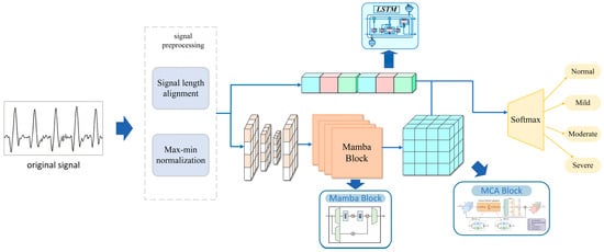
Figure 1. Overall design of the study.

2. Related Work

A shift from manual feature engineering to end-to-end paradigms has been documented in existing research, and the assessment of generalization, interpretability, and clinical utility remains a key challenge for future work. A single-channel SpO₂ signal is considered an attractive option for OSA screening because it is noninvasive and readily accessible. Recent AI-driven screening frameworks and systematic reviews have further emphasized the potential of overnight oximetry and other biosignals for OSA detection [4,5,6].

Early methods relied on handcrafted features such as the Oxygen Desaturation Index (ODI) and statistical descriptors, but their ability to generalize is limited. Recent breakthroughs in deep learning have been significant: OxiNet [7] is trained on 12,923 PSG records and achieved an AUC of 0.94 using only SpO₂ signals, reducing the missed diagnosis rate for moderate-to-severe OSA to 0.2%. An end-to-end model that does not require signal segmentation is proposed by Chen et al. [8]; It directly processes entire night SpO₂ sequences for four-level classification and achieves an accuracy exceeding 91%. However, the balance between instantaneous desaturation events and long-term trends is not yet adequately captured. Complementary information can be provided by multi-signal fusion, but system complexity is increased. An event detection accuracy of 94% is achieved by combining SpO₂ and respiratory flow signals with the Xception network [9]. A multi-scale Transformer that fuses ECG and SpO₂ and incorporates a cross-modal attention mechanism is proposed by Zhang et al. [10], achieving a three-class accuracy of 90%. However, multi-channel input and high computational overhead are required by these methods, limiting their applicability in home settings. Complementary to these approaches, Hoang and Liang proposed a multi-scale feature framework based on continuous wearable SpO₂ for OSA detection and severity classification, demonstrating the feasibility of fully wearable oximetry-based pipelines [11]. In addition, deep learning models using single-channel ECG have been reported for OSA severity detection, providing an important complementary biosignal modality [12].

The choice of sequence modeling architecture is directly tied to the ability to capture long-term dependencies. An accuracy of 92–94% is achieved on single lead signals by the CNN–LSTM hybrid network [8], but inference speed becomes a bottleneck when the sequence length reaches tens of thousands of time steps. Although the pure Transformer architecture has strong parallel computing capabilities, handling complete nighttime records is hindered by its quadratic complexity. The Mamba architecture is proposed in 2024 [13] and achieves linear time complexity through a state space model, providing a new paradigm for long sequence modeling. Bidirectional Mamba has been applied to sleep staging in MSSC BiMamba [14], but its application to OSA severity grading has not been fully explored.

In summary, existing methods have three key limitations: (1) reliance on signal segmentation leads to the loss of cross-segment information; (2) a single architecture is ill-suited to simultaneously model features across multiple time scales; and (3) balancing computational efficiency with accuracy for long sequence processing remains difficult. The research gap is addressed in this study by integrating Mamba’s efficient sequence modeling, LSTM’s long-term memory, and the hierarchical feature extraction capability of multi-scale convolutions to achieve end-to-end, four-level classification on complete SpO₂ sequences.

3. Materials and Methods

3.1. Proposed MSC-LSTM Model Structure

A parallel, multi-scale convolution-LSTM architecture with Mamba-based embeddings is proposed. As stated in the Introduction, traditional signal segmentation steps are not required; instead, the severity of OSA is classified into four levels directly. In addition, the proposed model is trained and evaluated directly on a publicly available dataset comprising a large number of SpO₂ recordings. As a result, high generalization is demonstrated, and accurate predictions on unseen data are achieved.

Figure 2 provides an overview of the proposed architecture. An overnight SpO₂ recording is first resampled or truncated to an 8 h window at 1 Hz, yielding an input sequence x (B × L × 1) with batch size B, sequence length L = 28,800, and a single channel. After OSA-aware adaptive smoothing and basic preprocessing, the normalized sequence is fed into two parallel branches: a deep multi-scale convolution–Mamba branch and a temporal LSTM branch.

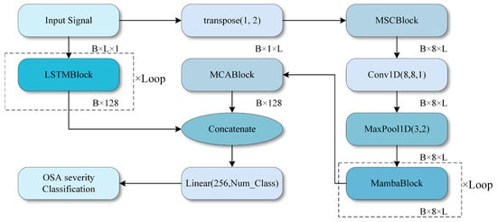
Figure 2. Overall structure of the study.

In the deep branch (Input Signal to MCABlock in Figure 2), three one-dimensional convolutional layers with kernel sizes 29, 59, and 179 are applied in parallel to the input sequence, producing feature maps of shape B × L × C_k at three temporal scales. These multi-scale feature maps are concatenated along the channel dimension and fused by a 1D convolution to obtain a unified representation B × L × C.

A stack of Mamba blocks then processes this representation to capture long-range temporal dependencies with linear-time complexity. Each Mamba block comprises layer normalization, the Mamba module, and residual connections, and it preserves the temporal length while increasing the channel dimension. The output of the deep branch is finally compressed along the temporal dimension by global pooling, resulting in a feature vector F_deep (B × D_deep).

In the temporal branch (LSTMBlock in Figure 2), the same preprocessed sequence x is fed into a six-layer LSTM with 128 hidden units per layer. The LSTM processes the entire 8 h sequence and outputs hidden states at each time step. The final hidden state of the top LSTM layer is used as a global temporal summary, resulting in a feature vector F_lstm with shape B × D_lstm. This branch is designed to explicitly capture long-term dependencies and slow trends in the SpO₂ signal.

The outputs of the deep branch and the LSTM branch are concatenated to form the fused feature F_fusion = [F_deep, F_lstm] (B × (D_deep + D_lstm). This fused feature passes through a multi-level channel attention module (MCA), which re-weights channels based on their statistical importance, and then through fully connected layers with non-linear activations. Finally, a Softmax layer produces the predicted probabilities for the four OSA severity levels.

The core architecture consists of several modules: Conv1D layers, a multi-scale convolutional network, Mamba blocks, an LSTM network, and a channel attention module (MCA1D_2) [15]. These components enable the model to capture temporal information and clinically relevant features more effectively than existing CNN-based OSA severity classifiers.

3.2. Model Structure Details

A SpO₂ signal of length 28,800 is provided as the input to the model, representing a complete 8 h monitoring sequence. The input shape is (28,800, 1). The input signal is preprocessed through signal smoothing, signal alignment, and missing value interpolation to ensure validity and is standardized as model input. All convolutional layers in Figure 3 are one-dimensional (Conv1D) layers used to extract features from time series signals.

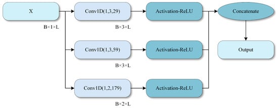
Figure 3. Multi-scale convolution module.

Specifically, the SpO₂ signal is provided as a one-dimensional sequence with an input shape of B × L × 1, where B denotes the batch size and L denotes the signal length. In the deep branch, a multi-scale convolutional network is first applied to extract multi-scale information using convolution kernels of sizes 29, 59, and 179.

The design of the convolution kernel sizes and the LSTM branch follow the temporal characteristics of OSA-related events. The three kernel sizes of 29, 59, and 179 (at a sampling frequency of 1 Hz) are chosen to cover complementary time scales that are clinically relevant. The smallest kernel (29 s) captures short-term fluctuations and rapid desaturation–reoxygenation cycles. The intermediate kernel (59 s) corresponds to the typical duration of apnea–hypopnea–related desaturation episodes of approximately one minute. The largest kernel (179 s) models slower baseline drifts over several minutes. Together, these scales align with the common duration range of OSA-related events and enable the network to represent both transient events and longer-term trends in the SpO₂ signal.

After the multi-scale convolution module, multiple Mamba blocks are concatenated to extract deep features from the SpO₂ signal. Temporal structure is efficiently modeled by the Mamba component, which captures long range dependencies and dynamic patterns. The input to each Mamba block is normalized and then processed by the Mamba network. Finally, key temporal information is preserved through gated fusion, thereby enhancing responsiveness to dynamic events such as desaturation. Next, multi-level channel attention weighting is applied by the MCA module to the extracted feature maps to enhance salient features.

In addition to the deep branch, an LSTM network is employed to model long-term dependencies in SpO₂ signals. The LSTM module effectively captures long-term trends and periodic variations, making it particularly suitable for physiological signals characterized by temporal dependencies. The LSTM network consists of six layers with 128 hidden units each, learning temporal patterns directly from the input signals. Features extracted from the deep branch and the LSTM branch are concatenated and fed into a fully connected layer for classification. The fused representation incorporates fine-grained spatial features extracted by the deep network and temporal features captured by the LSTM, enabling the model to exploit complementary information for more accurate classification. Finally, class probabilities corresponding to the four OSA severity levels are generated by a fully connected layer followed by a Softmax activation.

The detailed structure of MambaBlock, which includes layer normalization (LayerNorm) and a unidirectional Mamba module, is illustrated in Figure 4. MambaBlock captures long-term dependencies and dynamic changes in time series signals through efficient state space modeling and convolutional enhancement mechanisms. The fusion process of multi-scale convolution is depicted in Figure 3, in which three different-sized convolution kernels (29, 59, and 179) are used, and a 1D convolutional layer performs feature fusion.

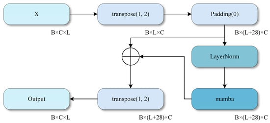
Figure 4. Mamba module. $⨁: \mathrm{A}\mathrm{d}\mathrm{d}$.

The operating principle of the MCA module is illustrated in Figure 5, where channel attention weights are generated by computing the mean and variance of each channel, thereby enhancing the model’s focus on key features. High classification performance is achieved through feature fusion and deep network learning across all modules.

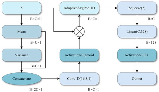
Figure 5. MCA module. $⨂: \mathrm{m}\mathrm{u}\mathrm{l}\mathrm{t}\mathrm{i}\mathrm{p}\mathrm{y}$.

For the LSTM branch, a six-layer LSTM with 128 hidden units per layer is employed to balance representational capacity and computational cost when processing sequences of up to 28,800 time steps. Preliminary experiments indicated that shallower LSTM architectures (e.g., two or four layers) exhibit inferior performance, suggesting insufficient capacity to encode long-range temporal dependencies. In contrast, deeper networks with more than six layers substantially increase training time and memory consumption, while providing only marginal performance gains. The adopted configuration therefore represents a practical compromise that offers adequate modeling power for full-night SpO₂ sequences without incurring prohibitive computational overhead.

3.3. OSA-Aware Adaptive Smoothing

During sleep monitoring, SpO₂ signals are extremely prone to interference from various types of noise, including motion artifacts, poor sensor contact, inadequate blood perfusion, and other factors.

Traditional signal smoothing methods typically use filters with fixed parameters, which creates a trade-off. Strong smoothing reduces noise but can attenuate or even remove genuine desaturation events, whereas weak smoothing preserves these events but does not sufficiently suppress noise. To tackle this issue, an adaptive smoothing algorithm for OSA perception (OSA-aware smoothing) has been developed. The key innovation of this algorithm is its capability to dynamically adjust the smoothing intensity based on the local characteristics of the signal, effectively removing noise while preserving the integrity of desaturation events. Initial signal cleaning is performed based on physiological knowledge. The physiological range of human blood oxygen saturation typically falls between 50% and 100%. Values outside this range are regarded as indicators of sensor malfunction or severe artifacts:

$$\begin{array}{c}\mathrm{M}\left(\mathrm{t}\right) = \{1, \mathrm{I}\mathrm{F} 50 \le {\mathrm{S}\mathrm{p}\mathrm{O}}_2(\mathrm{t}) \le 100; 0, \mathrm{E}\mathrm{L}\mathrm{S}\mathrm{E}\}\end{array}$$

(1)

$$\begin{array}{c}{\mathrm{S}\mathrm{p}\mathrm{O}}_2\_\mathrm{c}\mathrm{l}\mathrm{e}\mathrm{a}\mathrm{n}\mathrm{e}\mathrm{d}\left(\mathrm{t}\right)={\mathrm{S}\mathrm{p}\mathrm{O}}_2\left(\mathrm{t}\right) \times \mathrm{M}\left(\mathrm{t}\right)+\mathrm{I}\left(\mathrm{t}\right) \times (1 - \mathrm{M}\left(\mathrm{t}\right)),\end{array}$$

(2)

where M(t) represents a binary mask function, which takes the value of 1 when the SpO₂ level falls within the physiological range and 0 otherwise, and I(t) is an interpolation function employed to fill in invalid data points. The benefits of this processing approach are twofold: firstly, it preserves all physiologically plausible measurements, even if they are contaminated with noise; secondly, for conspicuous outliers (such as 0 or 255 values from equipment malfunctions), signal continuity is maintained by replacing them through interpolation rather than outright deletion, a practice that is vital for subsequent temporal analysis.

After eliminating outliers, a median filter with a small window (comprising 3 sampling points) is employed to remove pulse noise. Opting for a smaller window aims to prevent excessive smoothing of genuine rapid desaturation events. Pulse noise is characterized by its extremely brief duration (typically 1–2 sampling points) yet significant amplitude, whereas authentic desaturation events, even when occurring swiftly, necessitate a physiological process lasting at least 10–20 s. Consequently, median filtering using a 3-point window can effectively discern and eliminate isolated anomalies without impacting genuine physiological changes that persist for several seconds or more. The superiority of median filtering over mean filtering resides in its resilience to outliers; even in the presence of an extreme value within the window, the median remains stable while preserving the sharpness of signal edges.

Subsequently, compute the local variance at each time point as a metric for assessing the signal complexity in that specific region:

$$\begin{array}{c}\mathrm{L}\mathrm{s}\mathrm{d} \left(\mathrm{t}\right) = \mathrm{s}\mathrm{t}\mathrm{d}\left({\mathrm{S}\mathrm{p}\mathrm{O}}_2\right[\mathrm{t} - 30:\mathrm{t} + 30\left]\right)\end{array}$$

(3)

$$\begin{array}{c}\mathrm{N}\mathrm{o}\mathrm{r}\mathrm{m}\mathrm{C} \left(\mathrm{t}\right)=(\mathrm{L}\mathrm{s}\mathrm{d} (\mathrm{t}) - \mathrm{m}\mathrm{i}\mathrm{n}) / (\mathrm{m}\mathrm{a}\mathrm{x} - \mathrm{m}\mathrm{i}\mathrm{n})\end{array}$$

(4)

where Lsd represents the local standard deviation and NormC represents the normalization coefficient.

Regions with high variance typically correspond to desaturation events or recovery processes, and it is essential to retain details in these areas; conversely, regions with low variance usually represent stable baselines, where stronger smoothing can be applied.

Given the typical duration of sleep breathing events (ranging from 0 to 60 s), a 60 s window is chosen. This window size is sufficiently large to encompass complete breathing events, thereby enabling an accurate evaluation of local signal complexity. Based on this observation, an adaptive window mechanism is devised: a high σ value (>2%) generally signifies the occurrence of a desaturation event or recovery process, whereas a low σ value (<0.5%) indicates that the signal is in a stable baseline condition.

Next, normalize the local standard deviation to the [0, 1] range:

$$\begin{array}{c}\mathrm{\alpha }\left(\mathrm{t}\right) = (\mathrm{\sigma }\_\mathrm{l}\mathrm{o}\mathrm{c}\mathrm{a}\mathrm{l}(\mathrm{t}) - \mathrm{\sigma }\_\mathrm{m}\mathrm{i}\mathrm{n}) / (\mathrm{\sigma }\_\mathrm{m}\mathrm{a}\mathrm{x} - \mathrm{\sigma }\_\mathrm{m}\mathrm{i}\mathrm{n})\end{array}$$

(5)

where σ_min and σ_max represent the minimum and maximum local standard deviations of the entire signal, respectively. Normalization aims to ensure the algorithm’s consistent adaptability to OSA across different patients and varying severity levels. The closer the value of α(t) to 1, the higher the likelihood that the region contains significant clinical events.

Based on the normalization coefficient, an adaptive window size is designed:

$$\begin{array}{c}\mathrm{W}\_\mathrm{a}\mathrm{d}\mathrm{a}\mathrm{p}\mathrm{t}\mathrm{i}\mathrm{v}\mathrm{e}\left(\mathrm{t}\right) = \mathrm{W}\_\mathrm{b}\mathrm{a}\mathrm{s}\mathrm{e} + (1 - \mathrm{\alpha }(\mathrm{t}\left)\right) \times \mathrm{W}\_\mathrm{e}\mathrm{x}\mathrm{p}\mathrm{a}\mathrm{n}\mathrm{d}\end{array}$$

(6)

$$\begin{array}{c}\mathrm{W}\_\mathrm{b}\mathrm{a}\mathrm{s}\mathrm{e}=11, \mathrm{W}\_\mathrm{e}\mathrm{x}\mathrm{p}\mathrm{a}\mathrm{n}\mathrm{d}=20,\end{array}$$

(7)

when α(t) ≈ 1 (high complexity region), W_adaptive ≈ 11, and the details are preserved by the smallest window; when α(t) ≈ 0 (low complexity region), W_adaptive ≈ 31, and the sufficient smoothness is achieved by the maximum window.

Figure 6 shows the comparison of signals before and after smoothing.

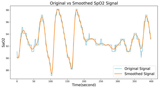
Figure 6. A comparison of signals before and after smoothing.

4. Experiment and Results Analysis

4.1. Data Sources

The publicly available Sleep Heart Health Study (SHHS) database [16] from National Sleep Research Resource (NSRR) [17] is used in this study. SHHS is primarily designed to evaluate the impact of sleep apnea on cardiovascular disease; specifically, the first examination (SHHS1; November 1995–January 1998) included 6441 participants aged 40 years or older, and the third follow-up (SHHS2; January 2001–June 2003) completed the second polysomnography (PSG) assessment [16].

A total of 5793 SHHS1 records are selected and split into training, validation, and test sets in a 70%/20%/10% ratio using stratified sampling to preserve the class distribution. SHHS2 is used only as an independent external test set, it is not involved in training, hyperparameter tuning, or model selection and underwent the same preprocessing as SHHS1. Table 1 shows the distribution and division of data sets used in this work.

Table 1. Shows the specific distribution of the dataset used.

Severity (AHI)	Training Set	Test Set
	SHHS1 (70%)	SHHS1 (10%)	SHHS2
Normal (AHI < 5)	702	100	475
Mild (5 ≤ AHI < 15)	1553	222	1020
Moderate (15 ≤ AHI < 30)	1108	159	703
Severe (AHI ≥ 30)	691	99	453
Total	4054	580	2651

4.2. Data Processing and Experimental Setup

Extracting SpO₂ channel signals from polysomnography (PSG) recordings, and samples are categorized as normal (AHI < 5), mild (5 ≤ AHI < 15), moderate (15 ≤ AHI < 30), or severe (AHI ≥ 30) according to the Apnea–Hypopnea Index (AHI). Figure 7 shows the comparison of SpO₂ signals between diseased and non-diseased patients

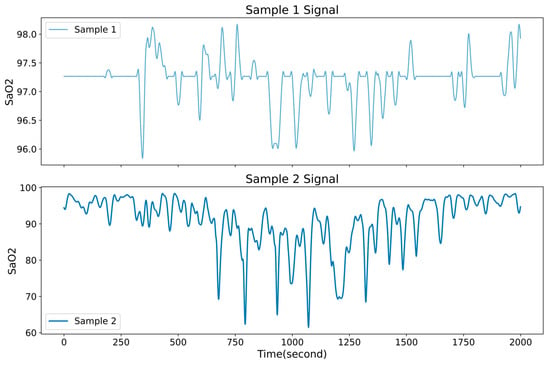
Figure 7. Comparison of SpO₂ signals between diseased and non-diseased patients.

Due to deep learning models require uniform sequence lengths, and recording durations vary substantially in SHHS1 (~3 to ~8.9 h), all SpO₂ sequences are truncated or zero-padded to 8 h at 1 Hz (8 × 3600 = 28,800 samples) and the sample sequences are denoised using OSA-aware adaptive smoothing (see Section 3.3 for details). Min–max normalization is applied to all SpO₂ signals, mapping values to the [0, 1] interval.

To address class imbalance, oversampling, undersampling, and the SMOTE (Synthetic Minority Over-sampling Technique) algorithm are employed to obtain a balanced distribution of samples across categories during training. The model is trained with a batch size of 64 for 200 epochs, using the cross-entropy loss and the Adam optimizer with an initial learning rate of 0.01 to improve training efficiency. Table 2 lists the development environment used in this study.

Table 2. The development environment used by the research institute.

Programing Language	Python 3.10
Library	Pytorch 2.1, Numpy 1.26, pandas 2.3, Mamba 2.2
Hardware	PC (Windows 11 64-bit, Intel Xeon Gold 6133 2.5 GHz CPU, 32 G RAM), graphics card (Nvidia Rtx A5000)

To avoid overfitting or training stagnation, a learning rate scheduler is used; when the validation loss failed to decrease for five consecutive epochs, the learning rate is halved until it reached 1 × 10⁻⁴, after which it is held constant. This procedure helped maintain stable convergence, with adjustments made when convergence bottlenecks occurred.

4.3. Evaluation Metrics

Model performance is evaluated by calculating four types of confusion matrices and calculating three metrics for each class: sensitivity, specificity, and accuracy. Class-wise averages for each metric and the overall accuracy are then computed, which is shown as:

$$\begin{array}{c}{\mathrm{Sensitivity}}_{\mathrm{i} }= {\mathrm{TP}}_{\mathrm{i}}/({\mathrm{TP}}_{\mathrm{i} }+ {\mathrm{FN}}_{\mathrm{i}})\end{array}$$

(8)

$$\begin{array}{c}{\mathrm{Specificity}}_{\mathrm{i}}={\mathrm{TN}}_{\mathrm{i}}/{(\mathrm{TN}}_{\mathrm{i}}+{\mathrm{FP}}_{\mathrm{i}})\end{array}$$

(9)

$$\begin{array}{c}{\mathrm{Precision}}_{\mathrm{i}}={\mathrm{TP}}_{\mathrm{i}}/({\mathrm{TP}}_{\mathrm{i}}+{ \mathrm{FP}}_{\mathrm{i}})\end{array}$$

(10)

Performance metrics, including sensitivity, specificity, and accuracy, are provided, where 1 ≤ i ≤ C = 4. These metrics are used to represent the i-th element of the prediction result classified into OSA severity levels {normal, mild, moderate, severe}; for example, i = 3 corresponded to moderate cases. True positives (TP) and false positives (FP) are defined as cases in which the predicted result is correctly or incorrectly classified as the i-th case, respectively. Similarly, true negatives (TN) and false negatives (FN) are defined as cases in which the predicted result is correctly identified as not belonging to the i-th case, or is incorrectly excluded from the i-th case, respectively.

Next, the average values and overall accuracy of the performance indicators in (1)–(3) are given by the following equations:

$$\begin{array}{c}\mathrm{M}\mathrm{e}\mathrm{a}\mathrm{n} = {\displaystyle \frac{{\sum }_{\mathrm{i}=1}^{\mathrm{C}}{\mathrm{x}}_{\mathrm{i}},\mathrm{x}\in \{\mathrm{Sensitivity}, \mathrm{Specificity}, \mathrm{Precision}\}}{\mathrm{C}}}\end{array}$$

(11)

$$\begin{array}{c}\mathrm{A}\mathrm{c}\mathrm{c}\mathrm{u}\mathrm{r}\mathrm{a}\mathrm{c}\mathrm{y}={\displaystyle \frac{{\sum }_{\mathrm{i}=1}^{\mathrm{C}}{\mathrm{TP}}_{\mathrm{i}}}{{\sum }_{\mathrm{i}=1}^{\mathrm{C}}({\mathrm{TP}}_{\mathrm{i}}+{ \mathrm{FN}}_{\mathrm{i}})}}\end{array}$$

(12)

Performance metrics include sensitivity, specificity, and accuracy. The F1-score is additionally reported to better account for class imbalance. For each OSA severity level i, the F1-score is defined as:

$$\begin{array}{c}{\mathrm{F}1}_{\mathrm{i}}={\displaystyle \frac{{2·\mathrm{P}\mathrm{r}\mathrm{e}}_{\mathrm{i}}·{\mathrm{S}\mathrm{e}\mathrm{n}}_{\mathrm{i}}}{{\mathrm{P}\mathrm{r}\mathrm{e}}_{\mathrm{i}}+{\mathrm{S}\mathrm{e}\mathrm{n}}_{\mathrm{i}}}}\end{array}$$

(13)

where Pre_i and Sen_i denote the precision and sensitivity of class i, respectively. The macro-averaged F1-score is obtained by taking the average of ${\mathrm{F}1}_{\mathrm{i}}$ for all classes.

To quantify the overall reliability beyond chance agreement, Cohen’s kappa coefficient (κ) is calculated between the predicted labels and the reference annotations. Let p_o denote the observed accuracy and p_e the expected accuracy by chance based on the marginal distributions of the confusion matrix; then

$$\begin{array}{c}\kappa ={\displaystyle \frac{p_o-p_e}{1-p_e}}\end{array}$$

(14)

where values of κ above 0.6 are generally interpreted as indicating substantial agreement, and values above 0.8 as almost perfect agreement.

Receiver operating characteristic (ROC) curves and the corresponding area under the curve (AUC) are also computed. In the four-class setting, a one-vs-rest strategy was applied. A separate ROC curve and AUC value were obtained for each severity level. For the binary experiments with AHI cutoffs of 5 and 15, ROC curves are generated for discriminating normal vs. apneic subjects at each threshold.

4.4. OSA Classification Results

In this study, a 10% subset of SHHS1 and the full SHHS2 cohort are used to evaluate the model’s four-class classification performance, as summarized in Table 3. The SHHS1 and SHHS2 test sets comprised 580 and 2651 records, respectively. The confusion matrices for the two datasets are presented in Figure 8 and Figure 9 to illustrate the test results.

Table 3. The proposed model OSA four-classification performance.

Test Set	Severity	Precision (Pre)	Sensitivity (Sen)	Specificity (Spe)	F1-Score	Accuracy (Acc)
SHHS1	Normal	0.7589	0.8500	0.9438	0.8019	0.8052
	Mild	0.7834	0.7658	0.8687	0.7745
	Moderate	0.7922	0.7673	0.9240	0.7796
	Severe	0.9278	0.9091	0.9855	0.9184
	Mean	0.8156	0.8230	0.9305	0.8186
SHHS2	Normal	0.8135	0.8358	0.9582	0.8245	0.7661
	Mild	0.8407	0.7088	0.9160	0.7691
	Moderate	0.6786	0.6999	0.8804	0.6891
	Severe	0.7249	0.9249	0.9277	0.8128
	Mean	0.7644	0.7926	0.9206	0.7739

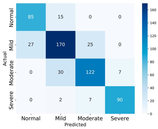
Figure 8. The Confusion Matrix of SHHS1.

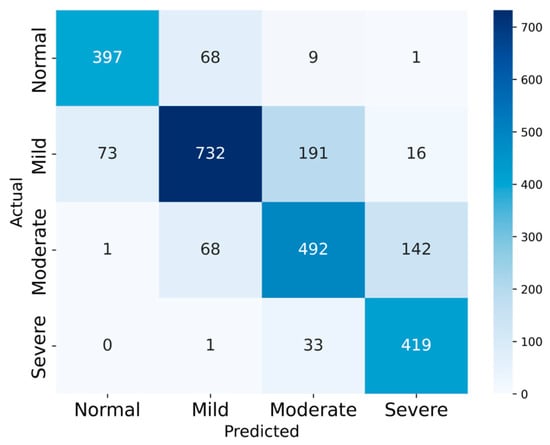
Figure 9. The Confusion Matrix of SHHS2.

On SHHS1, the model achieved 80.51% accuracy, with average sensitivity 81.98%, specificity 92.93%, precision 81.12% and F1-score 81.86%. On SHHS2, the corresponding values are 76.61%, 79.26%, 92.06%, 76.44%, and 77.39%, respectively.

For the four-class task, the macro-averaged F1-scores are 0.8186 on SHHS1 and 0.7739 on SHHS2, indicating balanced performance across the four severity levels despite the class imbalance. Cohen’s kappa coefficients are 0.729 and 0.687, respectively, corresponding to substantial agreement between the model predictions and the reference labels. These results suggest that the proposed model maintains good overall reliability beyond chance agreement.

Two sets of experiments are designed using AHI thresholds of 5 and 15 to examine the effect of these cutoffs on the performance of the proposed model, with the goal of enhancing its ability to distinguish normal signals from those of patients with apnea. Accordingly, the four OSA severity levels are collapsed into two categories: normal and apneic. Records with an AHI below the designated threshold are classified as normal, whereas those at or above the threshold are classified as apneic. Figure 10 and Figure 11 show the confusion matrices obtained from the experiment, respectively.

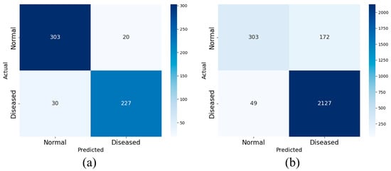
Figure 10. The binary confusion matrix with AHI = 5 as the cutoff in SHHS1 (a) and SHHS2 (b).

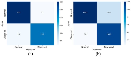
Figure 11. The binary confusion matrix with AHI = 15 as the cutoff in SHHS1 (a) and SHHS2 (b).

The test results are presented in Table 4. High overall accuracy is observed at both cutoffs. Using SHHS1 as an example, when the AHI threshold is set to 5, a diagnosis accuracy of 91.37% is achieved; the sensitivity, specificity, F1-Score, and accuracy are 93.81%, 88.32%, 92.38% and 90.99%, respectively.

Table 4. The proposed model OSA binary classification performance.

Test Set	AHI Cutoff	Precision (Pre)	Sensitivity (Sen)	Specificity (Spe)	F1-Score	Accuracy (Acc)
SHHS1	5	0.9099	0.9381	0.8832	0.9238	0.9137
	15	0.9152	0.9350	0.8911	0.9250	0.9155
SHHS2	5	0.9166	0.6379	0.9775	0.7523	0.9166
	15	0.9539	0.8033	0.9498	0.8721	0.8672

Figure 12 shows the one-vs-rest ROC curves for the four OSA severity levels on SHHS1 and SHHS2. The AUC values are 0.934, 0.871, 0.894, and 0.972 for the normal, mild, moderate, and severe classes, respectively. The high AUC for the severe classes indicate excellent discrimination between severe OSA and the remaining classes, while the slightly lower AUC for the mild class reflects the clinical overlap between normal and mild OSA.

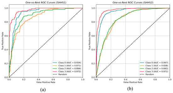
Figure 12. The one-vs-rest ROC on SHHS1 (a) and SHHS2 (b).

Similar trends are observed on SHHS2, with AUCs of 0.947, 0.838, 0.842, and 0.971 for the four classes, demonstrating that the proposed model maintains robust discrimination across datasets, particularly for moderate-to-severe OSA.

For the binary setting, as shown in Figure 13, the AUCs are 0.916 and 0.928 for AHI cutoffs of 5 on SHHS1 and SHHS2, respectively, and 0.965 and 0.950 for AHI cutoffs of 15. The consistently high AUC values indicate strong diagnosis performance in distinguishing normal from apneic subjects at clinically relevant thresholds.

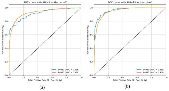
Figure 13. ROC with AHI = 5 (a) and AHI = 15 (b) as cutoff values.

4.5. Impact of OSA-Aware Adaptive Smoothing

To assess the contribution of OSA-aware adaptive smoothing, an additional set of experiments is conducted in which the adaptive smoothing step is replaced by alternative preprocessing strategies, while all other components of the pipeline remained unchanged. The following methods are compared:

Fixed median filter: a standard 11-point median filter applied uniformly to the entire SpO₂ sequence. This method uses a fixed window length for all regions, regardless of local signal variability, and thus represents a typical non-adaptive denoising strategy.

Butterworth low-pass filter: a 4th-order low-pass Butterworth filter applied to the SpO₂ signal. The cut-off frequency is chosen within the dominant frequency band of desaturation events, with the aim of attenuating high-frequency noise while preserving slower physiological fluctuations. The same cut-off parameter is applied globally over the whole recording.

Proposed OSA-aware adaptive smoothing: the full method described in Section 3.3, where the local standard deviation within a sliding window is used to adaptively adjust the effective smoothing window. High-variance regions, which usually correspond to desaturation events and recovery phases, are smoothed with a shorter window to preserve detailed morphology, whereas low-variance baseline segments are smoothed with a longer window for stronger noise suppression.

Each preprocessing variant is used to train and evaluate the complete MSC-Mamba-LSTM network on SHHS1 and SHHS2 under identical training and evaluation settings. Table 5 summarizes the performance in terms of overall classification accuracy (ACC). On SHHS1, accuracies of 0.7879, 0.7914, and 0.8052 are obtained for the fixed median filter, Butterworth low-pass filter, and OSA-aware adaptive smoothing, respectively. On SHHS2, the corresponding accuracies are 0.7602, 0.7533, and 0.7661, respectively. Thus, OSA-aware adaptive smoothing consistently achieved the best or near-best accuracy on both datasets, with absolute improvements of approximately 1–2 percentage points over standard fixed-parameter filters.

Table 5. Performance of different smoothing strategies on SHHS1 and SHHS2.

Signal Smoothing Strategies	Accuracy (Acc)
	SHHS1	SHHS2
Fixed median filter	0.7879	0.7602
Butterworth low-pass filter	0.7914	0.7533
OSA-aware adaptive smoothing	0.8052	0.7661

4.6. Ablation Experiment

In this study, the contributions of multi-scale convolution, the Mamba module, the MCA module, and the LSTM branch are systematically assessed by using ablation experiments. Overall, each component makes a positive contribution to performance across the two test sets, although some simplified variants achieve accuracy that is close to that of the full model on SHHS2.

As a baseline, a two-branch architecture comprising a conventional CNN and an LSTM was used, referred to as Model1. This configuration captures local features and temporal information, but its classification accuracy is significantly lower than that of the full model, which includes the additional modules.

In a subsequent ablation study, the multi-scale convolution module was replaced with a single-scale convolution (kernel size of 3), referred to as Model2. This modification diminished the model’s ability to capture features across multiple temporal scales, particularly when both high and low frequency components are present. As a result, recognition of complex patterns such as desaturation events and rapidly fluctuating SpO₂ signals degraded substantially, highlighting the necessity of multi-scale convolution for extracting frequency-specific information through hierarchical representations. The adverse effect is particularly pronounced for physiological signals characterized by complex dynamics.

Next, replacing the Mamba module with standard convolutional layers, referred to as Model3, saw a marked performance drop. The Mamba module captures temporal dependencies and dynamic changes in time series, enhancing the model’s responsiveness to rapid transitions or event-driven patterns. Without it, Model3 struggled to model these dependencies and underperformed on dynamic events (e.g., sudden desaturation). These findings highlight the Mamba module’s central role in modeling temporal relationships and trends.

In an additional ablation, the MCA module was removed, resulting in a variant referred to as Model4. The MCA module adaptively re-weights channel-wise features, enabling the network to emphasize salient information. In the absence of MCA, Model4 fails to highlight informative channels, thereby impairing the detection of segments pertinent to obstructive sleep apnea (OSA) severity. Therefore, MCA is critical for estimating feature importance in SpO₂ signals, particularly with multi-channel inputs, by directing attention to the channels most informative for classification.

Finally, eliminating the LSTM branch and retaining only the deep branch resulted in Model5, which substantially degraded overall performance. The LSTM branch captures long-term dependencies characteristic of physiological time series, particularly SpO₂. It enables the model to represent extended temporal context and periodic fluctuations. Without LSTM, Model5 fails to encode these long-range patterns, reducing sensitivity to long-term structure and lowering classification accuracy. Accordingly, LSTM is indispensable for modeling long-term dependencies and periodicity in temporal signals.

As a whole, these modules enhance multi-level feature extraction for complex physiological signals, yielding substantial gains in OSA severity classification. Each component contributes in a unique and complementary manner to overall performance. The results of the ablation experiment are listed in Table 6.

Table 6. Results of ablation experiment.

Models	Accuracy (Acc)
	SHHS1 (10%)	SHHS2
Proposed	0.8052	0.7661
Model1	0.7683	0.7432
Model2	0.7816	0.7287
Model3	0.7724	0.7612
Model4	0.7905	0.7491
Model5	0.7513	0.7634

These results indicate that each module complements the others in processing complex physiological signals (such as SpO₂), jointly improving the multi-level feature extraction ability and classification performance of the model. All experiments are conducted under the same training configuration.

It is noteworthy that on SHHS2 the accuracies of some ablated variants are very close to that of the proposed full model. These differences, which are within 0.3 percentage points, are comparable to the expected variability due to random initialization and data imbalance in SHHS2. In addition, although not shown in Table 6, the full model consistently yields higher sensitivity for moderate and severe OSA and more stable macro-averaged performance across classes indicating that the additional modules mainly improve robustness and class-wise balance rather than producing large gains in overall accuracy on every individual test set.

Furthermore, the pattern observed in Table 6 suggests a degree of redundancy and regularization among modules. Removing a single component can occasionally lead to a slightly higher accuracy on one dataset by reducing model capacity and mitigating overfitting, but this comes at the cost of reduced generalization to other datasets or OSA severity levels.

In summary, the ablation results support the conclusion that multi-scale convolution, Mamba, MCA, and LSTM provide complementary benefits, even though the numerical improvements in overall accuracy are modest for some ablated variants.

4.7. Results of Comparative Experiments

This section compares the proposed method with other sleep apnea syndrome identification methods explored in previous studies. Some previous works have demonstrated informative results. The comparison of the effectiveness of this method with better methods in classifying the severity of OSA in recent years is shown in Table 7.

Table 7. Comparison with other methods.

Works	Training Set	Test Set	Accuracy
This study	SHHS1 (70%, 4054)	SHHS1 + SHHS2 (3231)	0.8052
Ganglberger et al. [18] (2022)	private dataset (412)	private dataset (412)	0.7721
Chen et al. [8] (2023)	MESA + MrOS (5989)	SHHS (8444)	0.8051
Leino et al. [19] (2021)	HSAT (1970)	HSAT (197)	0.7875
Vaquerizo-Villar et al. [20] (2021)	CHAT + UofC + BUH (859)	CHAT + UofC + BUH (935)	0.6460

4.8. Interpretability Analysis Based on Grad-CAM

To enhance understanding of the model’s decision-making process and increase clinical trust, Gradient-weighted Class Activation Mapping (Grad-CAM) was applied to visualize the contribution of different temporal regions of the SpO₂ signal to the predicted class. The Grad-CAM scores with respect are computed to the final convolutional feature maps in the deep branch for correctly classified test samples.

Figure 14 shows a representative Grad-CAM heatmap for a case with ground-truth label “apneic” that is correctly classified by the model. The blue curve depicts the SpO₂ trajectory over time, and the color overlay indicates the Grad-CAM importance of each time point, with warmer colors (yellow–red) corresponding to higher contributions to the predicted class. As can be seen, regions with high Grad-CAM scores are tightly aligned with prominent desaturation events and their recovery phases, while stable baseline segments receive low scores. In particular, the model focuses on the onset and nadir of desaturations and on rapid re-oxygenation slopes, which are key clinical signatures of obstructive events. Across multiple test samples, similar patterns are observed. These observations are consistent with clinical expectations and indicate that the model captures physiologically meaningful patterns rather than spurious correlations.

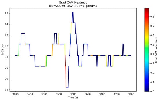
Figure 14. Grad-CAM heatmap for an SpO₂ segment from a correctly classified OSA patient. The blue line indicates the SpO₂ (%) over time, and the color overlay shows the Grad-CAM importance (higher values in yellow–red) for the predicted class.

5. Discussion

A multi-module deep network (multi-scale convolution, Mamba, MCA channel attention, and LSTM) is developed to classify OSA severity into four levels using a single-channel SpO₂ signal.

Overall accuracies of 80.51% and 76.61% are achieved on the SHHS1 and SHHS2 public datasets, respectively, while an average specificity greater than 92% is maintained, indicating effective control of false positives. Analysis of the four-class confusion matrices revealed that most misclassifications occurred between adjacent levels, a pattern consistent with gradual transitions around AHI thresholds in clinical practice, suggesting that the physiological features captured by the model reflect underlying pathophysiological changes. Compared with CNN-only SpO₂ classifiers reported in the literature (typically achieving 70–75% accuracy and often restricted to binary classification), higher-dimensional, fine-grained classification is achieved without signal segmentation, thereby demonstrating the advantages of end-to-end learning for complex temporal feature extraction.

The ablation experiments further quantified the contribution of each component: removing any module led to a marked decline in performance. In particular, when the Mamba or LSTM module is removed, the ability to capture sudden desaturation events and long-term trends is substantially weakened.

These findings indicate that temporal modeling and long-term dependencies are key factors in distinguishing mild, moderate, and severe OSA. It should be noted that although the average sensitivity exceeded 79%, it remained lower than the specificity (≈93%), indicating room for improvement in detecting true positive cases. First, SHHS2 contained a larger sample size but noisier signals, which reduced the model’s recall for moderate-to-severe cases. Second, although oversampling and SMOTE are used, class imbalance persisted in the training set. In future work, adaptive loss functions or adversarial resampling will be considered to further mitigate this issue.

The limitations of this study are as follows: (i) external validation and assessment of domain shift across multiple centers and devices are not performed; (ii) standardization on a per-record basis may attenuate inter-individual differences, and although robust quantile scaling is applied, additional population level validation is needed; (iii) the results require calibration and decision analytic evaluation of clinical net benefit; and (iv) the current model complexity remains high for edge device deployment. In future work, additional centers and devices will be included to form external cohorts, and distilled/quantized lightweight models together with prospective validation will be provided.

6. Conclusions

In this study, a deep network is constructed that integrates multi-scale convolution, Mamba, MCA channel attention, and LSTM, using publicly available large-scale SpO₂ data to perform a four-class automatic assessment of OSA severity. On the SHHS1 and SHHS2 test sets, accuracies of 80.51% and 76.61% and an average specificity greater than 92% are achieved; moreover, the contribution of each module to performance is corroborated through ablation experiments. A low-cost and scalable approach to home OSA screening is provided by this method, and a foundation is laid for future multimodal, real-time, and personalized sleep monitoring systems.

References

- Punjabi, N.M. The epidemiology of adult obstructive sleep apnea. Proc. Am. Thorac. Soc. 2008, 5, 136–143. [Google Scholar] [CrossRef] [PubMed]
- Dempsey, J.A.; Veasey, S.C.; Morgan, B.J.; O’Donnell, C.P. Pathophysiology of sleep apnea. Physiol. Rev. 2010, 90, 47–112. [Google Scholar] [CrossRef]
- Shojaee, A.; Mohsenin, V. Obstructive sleep apnea increases the risk of pulmonary hypertension independent of relevant risk factors. In Proceedings of the D19. SRN: Health Consequences and Outcomes of OSA: What do ‘Big Data’ and Clinical Trials Tell Us? Philadelphia, PA, USA, 15–20 May 2020; American Thoracic Society: New York, NY, USA, 2020; p. A6252. [Google Scholar]
- Hoang, N.H.; Liang, Z. AI-driven sleep apnea screening with overnight blood oxygen saturation: Current practices and future directions. Front. Digit. Health 2025, 7, 1510166. [Google Scholar] [CrossRef]
- Sabeenian, R.S.; Vinodhini, C.M. A Systematic Review on Machine Learning/Deep Learning Model-based Detection of Sleep Apnea Using Bio-Signals. Recent Pat. Eng. 2025, 19, E230724232158. [Google Scholar] [CrossRef]
- Singtothong, C.; Siriborvornratanakul, T. Deep-learning based sleep apnea detection using sleep sound, SpO2, and pulse rate. Int. J. Inf. Technol. 2024, 16, 4869–4874. [Google Scholar] [CrossRef]
- Levy, J.; Álvarez, D.; Del Campo, F.; Behar, J.A. Deep learning for obstructive sleep apnea diagnosis based on single-channel oximetry. Nat. Commun. 2023, 14, 4881. [Google Scholar] [CrossRef] [PubMed]
- Chen, J.W.; Liu, C.M.; Wang, C.Y.; Lin, C.C.; Qiu, K.Y.; Yeh, C.Y.; Hwang, S.H. A deep neural network-based model for OSA severity classification using unsegmented peripheral oxygen saturation signals. Eng. Appl. Artif. Intell. 2023, 122, 106161. [Google Scholar] [CrossRef]
- Yook, S.; Kim, D.; Gupte, C.; Joo, E.Y.; Kim, H. Deep learning of sleep apnea-hypopnea events for accurate classification of obstructive sleep apnea and determination of clinical severity. Sleep Med. 2024, 114, 211–219. [Google Scholar] [CrossRef] [PubMed]
- Zhang, Y.; Zhou, L.; Zhu, S.; Zhou, Y.; Wang, Z.; Ma, L.; Yuan, Y.; Xie, Y.; Niu, X.; Shi, Y.; et al. Deep learning for obstructive sleep apnea detection and severity assessment: A multimodal signals fusion multiscale transformer model. Nat. Sci. Sleep 2025, 17, 1–15. [Google Scholar] [CrossRef] [PubMed]
- Hoang, N.H.; Liang, Z. Detection and Severity Classification of Sleep Apnea Using Continuous Wearable SpO2 Signals: A Multi-Scale Feature Approach. Sensors 2025, 25, 1698. [Google Scholar] [CrossRef] [PubMed]
- Banluesombatkul, N.; Rakthanmanon, T.; Wilaiprasitporn, T. Single-channel ECG for obstructive sleep apnea severity detection using a deep learning approach. In Proceedings of the Tencon 2018–2018 IEEE Region 10 Conference, Jeju, Republic of Korea, 28–31 October 2018; IEEE: New York, NY, USA, 2018; pp. 2011–2016. [Google Scholar]
- Gu, A.; Dao, T. Mamba: Linear-time sequence modeling with selective state spaces. In Proceedings of the First Conference on Language Modeling, Philadelphia, PA, USA, 7–9 October 2024. [Google Scholar]
- Zhang, C.; Cui, W.; Guo, J. MSSC-BiMamba: Multimodal Sleep Stage Classification and Early Diagnosis of Sleep Disorders with Bidirectional Mamba. arXiv 2024, arXiv:2405.20142. [Google Scholar]
- Jiang, Y.; Jiang, Z.; Han, L.; Huang, Z.; Zheng, N. MCA: Moment channel attention networks. Proc. AAAI Conf. Artif. Intell. 2024, 38, 2579–2588. [Google Scholar] [CrossRef]
- Quan, S.F.; Howard, B.V.; Iber, C.; Kiley, J.P.; Nieto, F.J.; O’Connor, G.T.; Rapoport, D.M.; Redline, S.; Robbins, J.; Samet, J.M.; et al. The Sleep Heart Health Study: Design, rationale, and methods. Sleep 1997, 20, 1077–1085. [Google Scholar] [CrossRef] [PubMed]
- Zhang, G.Q.; Cui, L.; Mueller, R.; Tao, S.; Kim, M.; Rueschman, M.; Mariani, S.; Mobley, D.; Redline, S. The National Sleep Research Resource: Towards a sleep data commons. J. Am. Med. Inform. Assoc. 2018, 25, 1351–1358. [Google Scholar] [CrossRef] [PubMed] [PubMed Central]
- Ganglberger, W.; Bucklin, A.A.; Tesh, R.A.; Da Silva Cardoso, M.; Sun, H.; Leone, M.J.; Paixao, L.; Panneerselvam, E.; Ye, E.M.; Westover, M.B.; et al. Sleep apnea and respiratory anomaly detection from a wearable band and oxygen saturation. Sleep Breath. 2022, 26, 1033–1044. [Google Scholar] [CrossRef] [PubMed]
- Leino, A.; Nikkonen, S.; Kainulainen, S.; Korkalainen, H.; Töyräs, J.; Myllymaa, S.; Leppänen, T.; Ylä-Herttuala, S.; Westeren-Punnonen, S.; Myllymaa, K.; et al. Neural network analysis of nocturnal SpO2 signal enables easy screening of sleep apnea in patients with acute cerebrovascular disease. Sleep Med. 2021, 79, 71–78. [Google Scholar] [CrossRef] [PubMed]
- Vaquerizo-Villar, F.; Álvarez, D.; Gutiérrez-Tobal, G.C.; Arroyo-Domingo, C.A.; del Campo, F.; Hornero, R. Deep-Learning Model Based on Convolutional Neural Networks to Classify Apnea–Hypopnea Events from the Oximetry Signal. In Advances in the Diagnosis and Treatment of Sleep Apnea; Advances in Experimental Medicine and Biology; Penzel, T., Hornero, R., Eds.; Springer: Cham, Switzerland, 2022; Volume 1384. [Google Scholar] [CrossRef]
Disclaimer/Publisher’s Note: The statements, opinions and data contained in all publications are solely those of the individual author(s) and contributor(s) and not of MDPI and/or the editor(s). MDPI and/or the editor(s) disclaim responsibility for any injury to people or property resulting from any ideas, methods, instructions or products referred to in the content. |
© 2025 by the authors. Licensee MDPI, Basel, Switzerland. This article is an open access article distributed under the terms and conditions of the Creative Commons Attribution (CC BY) license (https://creativecommons.org/licenses/by/4.0/).